Challenges in Signal Analysis of Resonant-Mass Gravitational Wave Detectors
Nadja Sim˜ao Magalh˜aes
Centro Federal de Educac¸˜ao Tecn´ologica de S˜ao Paulo, Rua Pedro Vicente 625, S˜ao Paulo, SP 01109-010, Brazil and Instituto Tecnol´ogico de Aeron´autica - Departamento de F´ısica Pc¸a. Mal. Eduardo Gomes 50, S˜ao Jos´e dos Campos, SP 12228-900, Brazil
(Received on 15 October, 2005)
An overview of the main points related to data analysis in resonant-mass gravitational wave detectors will be presented. Recent developments on the data analysis system for the Brazilian detector SCHENBERG will be emphasized.
I. INTRODUCTION
As predicted by the theory of relativity and other theories of gravitation, time-dependent gravitational forces are expected to propagate in spacetime in the form of waves [1] . Such gravitational radiation is extremely difficult to detect because gravitation is the weakest of all the fundamental forces of na-ture.
For instance, a wave of very strong amplitude could gen-erate a displacement of 10−18m in a system (“antenna”) with typical length of 1m. In order to detect such a tiny displace-ment special sensors must be used and the signal should be sent to computers to be properly analyzed. The path between the antenna and the computer is tricky, though, because many spurious signals - noise - come as well.
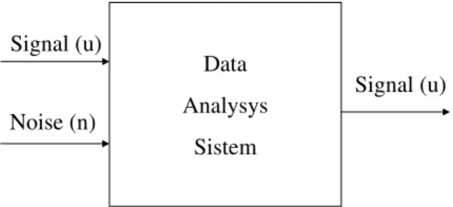
When an experiment is performed, normally the signal that is the object of the observation (the “useful” signal, u(t)) is accompanied by other, unwanted signals labelled with the generic name of “noise” (n(t)). The goal of signal analysis is to retrieve the useful signal out of noise, as illustrated in Figure 1. In the case of gravitational wave experiments, the useful signal is a gravitational wave.
Because signal analysis identifies the signal in the midst of the noise it becomes a fundamental part of the experiment. To do so it is necessary to know as much as possible about the signal and the sources of noise. In this work general features of data analysis in gravitational wave resonant-mass detectors will be presented, so that the reader can become familiar with the latest challenges faced by the Brazilian group that works
Data
Analysys
Sistem
Signal (u)
Noise (n)
Signal (u)
FIG. 1: The main objective of signal analysis is to retrieve the useful signal out of noise.
in the SCHENBERG gravitational wave detector within this important field.
This paper is organized as follows: in Section II the motiva-tion for the research is presented, namely gravitamotiva-tional waves and their sources. Section III is devoted to presenting gen-eral features of resonant-mass detectors, while Section IV dis-cusses some noises present in such detectors. Several basic concepts usual in the context of data analysis are presented in Section V while some important challenges that must be faced in the analysis of SCHENBERG’s data are discussed in Sec-tion VI. The closing comments are made in the final secSec-tion.
II. GRAVITATIONAL WAVE SOURCES
Strong gravitational waves (g.w.) are expected to be gen-erated by astrophysical objects [2]. For instance, two very massive stars orbiting each other would emit such waves. In particular, when they are coalescing they emit waves in a large frequency range. Another example is given by a black hole that rings down, also emitting in different wavelengths [3].
Astrophysical sources emit basically three kinds of waves, depending on the waveform: bursts (impulsive signals of short duration, like those produced by supernova explosions), con-tinuous waves (periodic, with long duration, like those emitted by stable binary systems) and stochastic waves (a spectrum composed with the superposition of many sources, as the one expected from cosmological origin).
From the analysis of the detected waves emitted by such sources important information is expected. The very first di-rect detection will provide a test for one of the predictions of the theory of general relativity. Then, continuous observation will allow testing other theories of gravitation [4, 5], besides initiating gravitational astronomy [6, 7].
In order to make astrophysical observations the following parameters that characterize the g.w. are needed: the ampli-tudes of the two states of polarization of the wave as func-tions of time (h+(t) andh×(t)), the source direction in the
FIG. 2: When a gravitational wave passes through a ring of particle it changes their relative positions, depending on the wave’s polar-ization. The top line shows the motion produced by a wave with polarization “+”, while the bottom line shows the motion due to a wave with polarization “×”.
the existence of such waves. All the existing detectors are presently aimed at this first detection, while being prepared to become part of g.w. observatories in the future as well. In the next section a brief overview on resonant-mass detectors will be presented.
III. RESONANT-MASS DETECTORS
When a gravitational wave passes through a ring of parti-cles it changes their relative positions [8], as shown in Figure 2. Similarly, solid bodies are distorted in the presence of such waves due to the changes in spacetime. This effect is the basis for resonant-mass gravitational wave detectors. For instance, a massive cylinder would oscillate longitudinally in the pres-ence of a g.w., in a frequency resonant with the wave.
The first of such detectors was built in the 1960’s by Joseph Weber. It was a massive, cylindrical aluminum bar at room temperature, 1.5m long, monitored by piezoelectric transduc-ers. Nowadays there are improved bar detectors, sometimes cooled down to millikelvin temperatures, longer and using more sensitive transducers [9]. Those that are operational at the moment are: ALLEGRO (EUA), EXPLORER (Switzer-land), NAUTILUS and AURIGA (both in Italy)
Bar detectors are able to determine only one observable, and due to their geometry there are directions in which they are more sensitive than others. For these reasons several bar detectors, appropriately positioned, would have to be used if one wished to build a gravitational observatory with only this kind of detector. In fact, investigations have already been done in this direction [10].
Besides cylindrical geometry, it has been known for some time that spherical, solid objects could be used as g.w. resonant-mass detectors. In principle this geometry has no preferred direction of observation (i.e., it is omnidirec-tional) and the five observables needed for gravitational
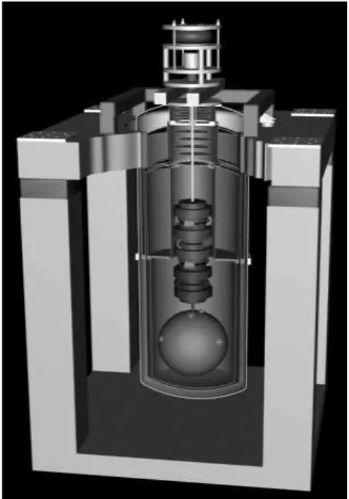
as-FIG. 3: Schematics of the SCHENBERG gravitational wave detector.
tronomy could be obtained from only one detector appropri-ately equipped [6, 11]. These are major advantages, but for many years bars were preferred because they were easier to machine and equip.
Under the rationale that spherical geometry is the best, in the last decade a lot of effort has been invested in investigat-ing and buildinvestigat-ing resonant-mass g.w. detectors with this design [9, 12]. The BrazilianMario SCHENBERGdetector is one of these last generation detectors [13] (see Figure 3). When fully operational it will be able not only to acknowledge the pres-ence of a g.w. within its bandwidth: it will be able to inform the direction of its source in sky, the wave’s amplitude and its polarization - one only antenna working as a gravitational wave observatory in a bandwidth between 3000 and 3400Hz, sensitive to displacements around 10−20m . To this end at least 6 transducers will continuously monitor displacements of the antenna’s surface. The data collected will be sent to be analyzed and, as mentioned above, it will certainly be accom-panied by some noise. In the next section some of the main noise sources in SCHENBERG will be presented.
IV. NOISE SOURCES IN SCHENBERG
Other kinds of noise are harder to minimize. The Brownian motion of the atoms of the antenna generatethermal noise, which can be reduced by cooling the massive sphere to tem-peratures as low as possible. SCHENBERG is expected to be cooled down to 4.2K (liquid Helium temperature) in its first test run. After the antenna is cooled down, the standard proce-dure to reduce its thermal noise has been to apply a threshold in the detected signal above which a signal may be considered a candidate for a g.w. event. It has been typical to set the threshold to amplitude signal-to-noise ratio between 3 and 5 [15]. In the future it is planned to cool SCHENBERG down to temperatures of the order of millikelvin, decreasing the an-tenna’s thermal noise in about one order of magnitude [16].
Other relevant noises in SCHENBERG are related to the transducers used to translate the mechanical motion of the an-tenna into an electrical signal. They are microwave parametric transducers [17] that generate noises that can be divided into two groups: narrow band and broadband noises. The narrow band noise includes the back action and the Brownian noises. The broadband noise can be divided into two components: one due to the amplifier and another due to the phase noise in the pump microwave source. All these noises have been modelled mathematically [16] so that the corresponding expressions can be used in the development of digital filters that help to mini-mize these noises in the detected signal. The importance of the determination of such mathematical expressions will become more clear within the context of data analysis, as follows.
V. BASIC CONCEPTS IN DATA ANALYSIS
The electric signal that leaves the transducers carries infor-mation of both the gravitational wave and the different noises. Data analysis then tries to extract the g.w. signal as clean as possible out of noise. In other words, one is concerned with improving the signal-to-noise ratio of measurements: an ac-curate measurement can be made when the g.w. signal causes an output of the detector that is large compared to the random variations of the output when no g.w. signal is present. In what follows some basic concepts important do data analysis will be presented, including signal-to-noise ratio. The theory of signal detection, much of it invented in the context of the development of the radar during World War II, can be found in a number of books [18, 19].
The output of a g.w. detector is expected to be continuously recorded, and this allows one to know this output as a func-tion of time: s(t). Such mathematical object is called atime series. In principle one hopes to know as much of the g.w. signal as possible, making it a deterministic time series of a predetermined form,u(t), or atemplate. For instance, burst signal are commonly associated to Dirac’s delta function. On the other hand, noise is usually associated to time series,n(t), that randomly varies from one realization to the next. Before data analysis one then hass(t) =u(t) +n(t). Notice that in the absence of any g.w. signal the detector output is just plain noise:s(t) =n(t).
These distinctions between the time series of the g.w. signal and noise imply different mathematical operations to
charac-terize the regularities of these series. A useful way to express the time series is in terms of its Fourier transform, S(f), a function of frequency which contains the same information of the time seriess(t), defined by
S(f)≡√1 2π
Z ∞
−∞s(t)e −2πf t
dt.
This puts the data in thefrequency domain. Notice that since data is sampled in discrete sets in the practical world, the dis-crete analog of the above equation is a more appropriate way to define the Fourier transform for real data sets. In fact, there exists a powerful algorithm for calculating discrete Fourier transforms, the FFT or Fast Fourier Transform, which is very useful in modern laboratory instrumentation. But for this brief presentation of the subject the continuous approach will be preferred.
The value of the Fourier transform ofs(t)at the frequency f is a measure of the degree to whichs(t)varies like a sinu-soid of frequency f. Putting it in a better way, the Fourier transform gives the contribution of a sinusoid of frequency f to a sum of sinusoids that equals the function of interest,s(t) in this example.
For a deterministic signal as the one expected for g.w. its Fourier transform can be calculate quite straightforwardly from the above definition. The characterization of a random time series (noise) in the frequency domain demands an extra step, which is the definition of theautocorrelation functionof the noise:
n∗n(τ)≡
Z ∞
−∞n(t)n(t+τ)dt.
This function of a time offsetτis a way of measuring hown(t) is related to itself, at different time offsets between two copies ofn(t). Whenτ=0 the time series is aligned to itself so the autocorrelation function will always have a maximum at this time offset. The width ofn⋆nindicates how rapidly the noise changes with time.
The translation of the random time seriesn(t)into the fre-quency domain is then given by the thepower spectrumof this series (also known as power spectral density), defined as the Fourier transform of the autocorrelation function:
Ps(f)≡ 1 √
2π Z ∞
−∞n∗n(τ)e
−2πfτdτ.
Ps(f)is a measure of the amount of time variation in the time series that occurs in the specific frequency f.
Instead of thinking in terms of complex integrals of both positive and negative frequencies, experimentalists often pre-fer to think in terms of sines and cosines of positive frequen-cies. So it is common to use thesingle sided power spectrum, s2(f), defined by
s2(f)≡ ½
2Ps(f), i f f ≥0 0, otherwise.
from this quantity is commonly used, theamplitude spectral density, defined simply bys(f)≡p
s2(f). Details on the
ad-vantages and disadad-vantages of the use of these quantities can be found in [20].
After presenting how signal and noise can be characterized in the theory of signal detection, now the concept of signal-to-noise ratio (or SNR) will be introduced. This is a dimension-less figure of merit for a measurement. In order to create such a dimensionless quantity one must keep in mind that signal detection is the process of searching for a pattern resembling the template in the middle of a noisy record. Such a pattern should occur with a strength unlikely to be due to noise alone. The match between the time record and the template can be estimated by thecross-correlation integralbetween the tem-plate u(t)and the time records(t), evaluate for all possible times at which the signal could have arrived:
s∗u(t)≡
Z ∞
−∞s(τ)u(t+τ)dτ.
This definition is similar to the definition of the autocorrela-tion funcautocorrela-tion, given previously. The cross-correlaautocorrela-tion func-tion indicates how related the funcfunc-tions s(t)andu(t)are to each other. Then one way to characterize the strengthS2of
the signal present in any timet is using the cross-correlation between the expected form of the output (the templateu(t)) and the outputs(t):
S2≡ |s∗u(t)|.
As for the noise, it can be characterized byN2, the mean square value of the cross-correlation between the outputs(t) in the absence of g.w. (i.e., noise) and a given template:
N2≡D(s∗u(t))2E.
The bracketshiindicate averaging over time.
With these characterizations one defines the signal-to-noise ratio as the square root of the ratio of the measure of the amount of signal present (S2) to the expected value due to noise alone (N2):
SNR≡qS2± N2.
A large SNR indicates that something is present in the time series s(t) other than noise. In practiceSNR≈1 is not of much use, but SNR&10 indicate detection of some confi-dence. Therefore the goal is to maximize SNR in order to detect a g.w. This can be accomplished in a number of ways. For instance,n(t)for antenna’s thermal noise can be reduced by cooling the antenna down. As for transducer’s noise, a dig-ital filter is useful. Filtering is such an important part of signal analysis that it will be briefly reviewed next.
Suppose there is a device possessing one single input (i(t)) and a single output(s(t)). Such device will be considered a linear systemif there is some linear relationship between the input and the output:s(t) =a i(t). When the relationship be-tween the input and the output does not change with time,
then the device is alinear time-invariant system(or just linear system for short).
Thefiltersconsidered here are linear time-invariant devices in which the input and output are quantities with the same dimensions. On the other hand, the termtransduceris used as a general name for a linear system whose input and output have different physical units.
One way to specify the input-output relationship in a linear system is to give the “impulse response”,g(t). This function is the output obtained when a single unit impulse is applied to the input att=0. In the frequency domain the Fourier trans-form of the impulse response,G(f), is called thefrequency response(or sometimestransfer function). This is a complex-valued function of the frequency f whose real part represents the response “in phase” with a sinusoidal input of frequency f, while the imaginary part corresponds to the “quadrature” component. One can show that ifI(f)is the Fourier trans-form of the input andS(f)is the Fourier transform of the out-put, thenG(f) =S(f)/I(f). This equation implies also that in Fourier space the output of a linear system is simply the product of the input and the frequency response, with no need to calculate convolution integrals.
VI. ASPECTS OF SCHENBERG’S DATA ANALYSIS
The theory presented in the last section shows that the knowledge of SNR for SCHENBERG demands the determi-nation of the time series of: the detector’s output, the g.w. signal (template) and the noise.
In the particular case of SCHENBERG it is necessary to combine the outputs of several transducers to create the time series of the output,s(t). This combination is part of the math-ematical modelling of the detector. There are 6 transducers planned to monitor the antenna surface’s motion and there are mathematical models for the detector for the case that all these transducers operational. Such models have investigated two situations: one in which the transducers are perfectly uncou-pled [11, 21, 22] and another in which the transducers are somehow coupled to each other [23], an instance that still of-fers possibilities of investigation.
One of the challenges presently faced by the data analysis group within the GRAVITON project [24] (the one SCHEN-BERG is part of) is to develop a model of the detector with less than 6 transducers. In this case there is a break in the convenient buckyball symmetry [21] and the consequences of this fact must be investigated. Two approaches are now un-der investigation: one consiun-ders the model already developed for 6 transducers [25] and simply reduces their number; the other considers the fewer transducers as independent devices and redesign the mathematical model. For the study of the last approach several references in the literature may be used as a starting point [26–30].
An actual time series of the detector’s output is expected be known as soon as it is collecting data, in the next months. At least three transducers are expected to be installed then, so the investigation mentioned above should be conclude soon.
tem-plate has started long ago and is one of the more active fields in data analysis [31], so that several templates already exist that can be used [3, 32, 33]. But still many challenges re-main to be faced in the field of g.w. sources. At the moment one of the investigations been carried out by SCHENBERG’s data analysis group in this way refers to the detection of astro-physically unmodelled bursts of gravitational radiation using wavelets [34].
A significant work has already been done to determine the time series of the noise in SCHENBERG, as mentioned in Section IV. Since all time series needed are available one is able to translate them into the frequency domain and deter-mine SCHENBERG’s SNR, as is done in [3]. Also, based on the model with 6 transducers operational simulations of the detector in the presence of noise have already been made (see Costa and Aguiar in [9]).
The improvement of SNR can be accomplished by using appropriate digital filters, for instance. When noise is white (broadband, spread over spectrum and stationary, implying a spectral density that does not depend on the frequency, which is commonly the case) it can be shown that the best filter for a given template is thematched filter. This linear system has an impulse response which is the time reverse of the signal one is interested in: g(t) =s(−t). This filter is presently under investigation for the case of SCHENBERG within GRAVI-TON’s data analysis group.
When noise is not white (either by not being broadband nor stationary, or both) other strategies are used. For instance, the monitoring of the environment with seismographers help vetoing seismic noises. Monitors for cosmic rays work simi-larly. The possible influence of lightings on the data has been investigated as well (see Magalhaes, Marinho, Jr. and Aguiar in [9]).
In the particular case of SCHENBERG, which will be mon-itored by several transducers simultaneously, one may wonder if filtering should be performed at the transducers outputs to veto non-white, non-stationary noise before combining them to extract the wave’s parameters. This is the case when sev-eral bar detectors work in coincidence [15], spaced around the world with some different characteristics among themselves. Maybe such a procedure would eliminate some noise due to local disturbances in individual transducers so that the com-bined data could be less noisy.
However it can be argued [35] that since SCHENBERG’s identical transducers are collecting data simultaneously at the same site there is no need to risk loss of information by fil-tering their data before combining them, a combination that will be possibly done in real time and with all characteristics under control. The data analysis system is then expected to be able to optimize SNR using the combined outputs without intermediate filtering.
Besides the matched filter another kind of filter is under investigation for SCHENBERG, namely anadaptative filter, one that changes with the variations of the power spectrum
of the noise. This is a device useful in the presence of non-stationary noise, like electric and seismic noises. This kind of filter has already been investigated within the g.w. detection context [36].
Finally, an aspect that still deserves investigation is the use of the Bayesian statistics in SCHENBERG’s data analysis. Such kind of study is already been carried out related to other detectors (see L.S. Finn in [9]).
VII. CONCLUDING REMARKS
In this work a brief overview of data analysis in resonant-mass gravitational wave detectors was presented, with empha-sis on issues involving the SCHENBERG detector. This de-tector, installed at the Physics Institute of the University of Sao Paulo (Sao Paulo city), is expected to be collecting data soon. It will be able to run in coincidence with other detectors around the world, particularly the broadband interferometric ones (see links for the several groups at [24]). Such kind of coincidence is important in the first place to increase the cred-ibility on the detection of a g.w. For this reason it is interesting to consider the development of a common protocol for infor-mation exchange between SCHENBERG and these detectors. It is worth pointing out the particular feature of SCHEN-BERG of working as an observatory of g.w. by itself due to its capability of several simultaneous measurements. Moni-tored by three transducers, as it is planned for the near fu-ture, this detector will be able to determine the squared ampli-tude and the direction of propagation of a g.w. sufficiently strong within its frequency band. Only spherical detectors like SCHENBERG are able to have such versatility. This is the case of the MiniGrail, another spherical detector built in The Netherlands (see de Waard in [9]) sensitive to frequencies smaller than SCHENBERG’s. Also, an Italian group is inter-ested in building a large spherical detector (see V. Fafone in [9]).
There is the belief within the international community that works with g.w. detection that the first direct detection of gravitation radiation from an astrophysical source will be-come a reality in the near future. This will open a new window to the universe, bringing new information about known ob-jects and about fairly unknown things, like dark matter. In or-der to extract such information from the huge amount of data that is expected to be generated from the detectors’ outputs (which has already started) a lot of work will be demanded in the field of data analysis. This is a promising field.
Acknowledgements
The author is thankful to Odylio D. Aguiar for kindly al-lowing the reproduction of Figure 3.
[2] K.S. Thorne, in300 Years of Gravitation, eds. S. W. Hawking and W. Israel. Cambridge: Cambridge Univ. Press, 1987. [3] C. A. Costa, O. D. Aguiar and N. S. Magalhaes,Class.
Quan-tum Grav.21,, S827 (2004).
[4] N. S. Magalhaes, W. W. Johnson, C. Frajuca, and O. D. Aguiar, “The detection of gravitational waves as a test for theories of gravitation”. Proceedings of the XVII Brazilian Meeting on Par-ticles and Fields (Serra Negra, Brazil, 1996). S˜ao Paulo: SBF, 202.
[5] S. M. Merkowitz,PRD58, , (062002).1998
[6] N. S. Magalhaes, W. W. Johnson, C. Frajuca, and O. D. Aguiar, MNRAS274, 670 (1995).
[7] B. F. Schutz, ”Physics and Astrophysics of Gravitational Waves”. Notes to lectures at Cardiff University (February, 2005), available at “www.aei.mpg.de”.
[8] B.F. Schutz,A First Course in General Relativity, Cambridge: Cambridge Univ. Press, 1990.
[9] Latest news on g.w. detectors can be found at the 6th Amaldi Conference on Gravitational Waves homepage at “www.amaldi6.nao.ac.jp”.
[10] More information on the network of bar detectors can be found at theInternational Gravitational Event Collaboration(IGEC) homepage: “igec.lnl.infn.it”.
[11] N. S. Magalhaes, O. D. Aguiar, W. W. Johnson and C. Frajuca, Gen. Relat. Grav.29, 1511 (1997). And references therein. [12] V. F. Velloso, Jr., O. D. Aguiar and N. S. Magalhaes, editors,
Proceedings of the First International Workshop Omnidirec-tional GravitaOmnidirec-tional Radiation Observatory, Singapore: World Scientific, 1997.
[13] See O. D. Aguiar et al. in these proceedings.
[14] O. D. Aguiar et al.,Class. Quantum Grav.19, 1949 (2002). [15] IGEC ,Phys. Rev. D68, 022001 (2003).
[16] C. Frajuca et al.,Class. Quantum Grav.21, S1107 (2004). [17] L.A. Andrade et al.,Class. Quantum Grav.21, S1215 (2004). [18] A.D. Whalen,Detection of Signals in Noise, New York:
Acad-emic, 1971.
[19] L.A. Wainstein and V.D. Zubakov,Extraction of Signals from Noise, New York: Dover, 1970.
[20] P.R. Saulson, Fundamentals of Interferometric Gravitational Wave Detectors, Singapore: World Scientific, 1994.
[21] S.M. Merkowitz and W.W. Johnson, Phys.Rev. D 56, 7513 (1997).
[22] C.A. Costa,PhD Thesis(in Portuguese), Sao Jose dos Campos: INPE, 2005.
[23] S.M. Merkowitz, J.A. Lobo and M.A Serrano,Class. Quantum Grav.16, 3035 (1999). And references therein.
[24] The homepage of the GRAVITON project is at “www.das.inpe.br/∼graviton”.
[25] C.A. Costa,Master Dissertation(in Portuguese), Sao Jose dos Campos: INPE, 2002.
[26] G. Pizzela,Il Nuovo Cim.102B, 471 (1988).
[27] Y. G¨ursel and M. Tinto,Phys. Rev. D40, 3884 (1989). [28] M. Cerdonio et al.,Phys. Rev. Lett.71, 4107 (1993). [29] C.Z. Zhou and P.F. Michelson,Phys. Rev. D51, 2517 (1995). [30] A. Pai, S. Dhurandhar and S. Bose,Phys. Rev. D64, 042004
(2001).
[31] Latest news on data analysis for the detection of g.w. can be found at the9th Gravitational Wave Data Analysis Workshop homepage at “lappweb.in2p3.fr/GWDAW9/Program.html”. [32] O.D. Aguiar et al.,Class. Quantum Grav.21, S457 (2004). [33] J.C.N. de Araujo et al.,Class. Quantum Grav.21, S521 (2004). [34] See N.S. Magalhaes and R.M.Marinho, Jr. in XXVI En-contro Nacional de Fisica de Particulas e Campos at “http://www.sbf1.sbfisica.org.br/eventos/enfpc/xxvi /sys/resumos/R0240-1.pdf”.
[35] O.D. Aguiar, private communication.