Multiple Charging Station Location-Routing Problem with Time Window of Electric Vehicle

Journal of Engineering Science and Technology Review 8 (5) (2015) 190 - 201

Research Article

Multiple Charging Station Location-Routing Problem with Time Window of Electric

Vehicle

Wang Li-ying and Song Yuan-bin*

School of Naval Architecture, Ocean and Civil Engineering, Shanghai Jiao Tong University, Shanghai 200240, China

Received 19 August 2015; Accepted 11 November 2015

___________________________________________________________________________________________

Abstract

This paper presents the electric vehicle (EV) multiple charging station location-routing problem with time window to optimize the routing plan of capacitated EVs and the strategy of charging stations. In particular, the strategy of charging stations includes both infrastructure-type selection and station location decisions. The problem accounts for two critical constraints in logistic practice: the vehicle loading capacity and the customer time windows. A hybrid heuristic that incorporates an adaptive variable neighborhood search (AVNS) with the tabu search algorithm for intensification was developed to address the problem. The specialized neighborhood structures and the selection methods of charging station used in the shaking step of AVNS were proposed. In contrast to the commercial solver CPLEX, experimental results on small-scale test instances demonstrate that the algorithm can find nearly optimal solutions on small-scale instances. The results on large-scale instances also show the effectiveness of the algorithm.

Keywords:Electric vehicles, Vehicle routings, Location-routing problem, Green logistics, Hybrid metaheuristics

__________________________________________________________________________________________

1. Introduction

With the increasing worldwide concern on the environment, the negative effects of logistic operations, particularly in terms of greenhouse gas emission, can no longer be neglected. Electric vehicles (EVs), powered by the reproducible resource, are currently considered to be a crucial alternative to conventional internal combustion vehicles (ICVs) to improve the sustainability of logistic operation. In contrast to ICVs, EVs have both environmental and economical advantages [1]. Several industries have started to use EVs for distribution operation in recent years, such as the consumer goods industry [2,3]. In addition, the logistic giant, DHL, has engaged more than 304 EVs for delivery activities and plans to adopt 140 EVs for delivery tasks in Bonn/Germany by 2016 [4].

In planning last-mile delivery task with EVs, the potential requirement of charging en route resulting from limited battery capacity should be rendered. Given the deficiency of public charging stations and the requests of logistic operations, such as time-definite deliveries, it’s regarded as a promising alternative that the logistic enterprise operates its own charging stations [6].

Several types of charging infrastructure exist in practice, and each has its pros and cons. For example, although the battery swap station (BSS) can provide faster service than other types of charging stations, the establishment cost of BSS is much higher than that of others [5]. The infrastructure-type decision of a station has a great effect on

the location decision of the station and the routing plan of EVs, while it is swayed by the location of the station and routing plan. The location of the charging station also has a great influence on the routing plan of EVs, and the routing plan of EVs is a key factor to locate charging stations [6]. Thus, these three problems should be addressed simultaneously to obtain an optimal solution. Two constraints of last-mile delivery practice, that is, customer time windows and vehicle loading capacity, are also critical for the routing plan and should be incorporated into the problem [7]. The time window constraint is quite interesting because the recharging time for an EV is determined by both the charging infrastructure and the distance traveled from the last charging station, and the arrival time at the customer after a visit is affected by the charging time in the preceding station and is restricted by the time window.

This study introduces the EV multiple charging station location-routing problem with time window (EV-MCS-LRPTW). The problem incorporates the location decision and the type selection of charging infrastructure with the vehicle-routing plan，and considers customer time windows and the loading and battery capacities of vehicles. Each type of charging infrastructure is associated with a particular construction cost and charging rate. The problem is intended to provide an optimal solution with a minimal cost for the logistic enterprise that plans to adopt EVs for distribution and to construct its own charging stations. The problem minimizes the total cost, including the construction cost of the charging station, the charging cost of EVs, and the labor cost of drivers. Given that the problem extends the location-routing problem (LRP), exact solution methods are incapable of addressing realistically sized instances within reasonable time periods [8]. Thus, we develop a hybrid heuristic named adaptive variable neighborhood search (AVNS)/tabu search (TS) to solve the problem, which

______________

* E-mail address:ybsong@sjtu.edu.cn

ISSN: 1791-2377 © 2015 Kavala Institute of Technology. All rights reserved.

J

estr

JOURNAL OF Engineering Science

and Technology Review

integrates an AVNS heuristic with the TS algorithm for intensification. The AVNS algorithm incorporates the adaptive idea from the adaptive large neighborhood search (ALNS) into the variable neighborhood search (VNS) framework to bias the random shaking phase of VNS. The performance of AVNS/TS is tested on several sets of instances in numerical studies. Experiments on small-scale instances are used to evaluate the solution quality of AVNS/TS, and tests on large-scale instances are adopted to assess the effectiveness of the algorithm.

The remainder of this paper is organized as follows: Section 2 briefly reviews the literature related to EV-MCS-LRPTW. Section 3 illustrates the mathematical formulation of the problem. Section 4 provides the solution approach. Section 5 demonstrates the parameter setting, the generation of new E-MCS-LRPTW instances, and the numerical studies. Finally, Section 6 concludes the study and summarizes the future works.

2. Related background

In this section, we review the literature related to EV-MCS-LRPTW. Two streams of previous studies are most relevant to the present research. One is the LRP, and the other is the routing planning of alternative fuel vehicles (AFVs).

2.1 Location routing problem

A network is normally represented by a graph that is composed of a set of nodes and edges. The task of network clustering is to divide a network into different clusters based on certain principles. Each cluster is called a community. The LRP combines two classical planning tasks in logistics, that is, optimally locating depots and planning vehicle routes from these depots to geographically scattered customers [8]. These two interdependent problems have been addressed separately for a long time, which often leads to suboptimal planning results. The idea of LRP started in the 1960s, when the interdependence of the two problems was pointed out [9,10]. The variants of the LRP have been frequently studied in recent years. Such variants include the capacitated LRP (CLRP) with constraints on depots and vehicles [20,21], the LRP with multi-echelon of networks [11,12], the LRP with inventory management [13,14], and the LRP with service time windows [15–17]. For the variant problem with time windows, Semet and Taillard incorporated the time window constraint to the LRP for a special case of the road–train-routing problem [15]. Zarandi et al. studied the CLRP with fuzzy travel time and customer time windows, in which a fuzzy chance-constrained mathematical program was used to model the problem [16]. Later, they extended the problem by adding the fuzzy demands of customers and developed a cluster-first route-second heuristic to solve the problem [17]. A detailed review of the LRP variants can be found in two recent surveys [18,19].

For the solution method of LRP, studies that focus more on heuristics than on exact methods have been observed in the existing literature probably, because the LRP combines two nondeterministic polynomial-time-hard problems. Most of the heuristic methods can be classified into two categories. One category commonly applies modified metaheuristics to improve the initial solution generated in a previous step. For instance, to solve the CLRP, Jokar and Sahraeian first applied a greedy approach to produce an initial solution and then proposed the simulated annealing (SA) algorithm to exploit better solutions from the initial solution [20].

Hemmelymay et al. applied their ALNS metaheuristic enhanced by a local search algorithm in improving the initial solution to address the CLRP [21]. The other category is executed first by separating the LRP into two sub-problems—the vehicle-routing problem (VRP) and the facility location problem—and then by solving the sub-problems sequentially or iteratively. Perl and Daskin first proposed the idea of iterating between locational and routing phases, and the idea has been improved in several studies later [22].

2.2 Routing problem of alternative fuel vehicles

The second strand of the relevant literature consists of the routing problems that consider the limited driving range of vehicles and the possibility of refueling en route. Conrad and Figliozzi introduced the recharging VRP, in which vehicles with a limited range are allowed to recharge at certain customer stations within a fixed time [23]. Erdogan and Miller-Hookers presented the green VRP (G-VRP) for routing AFVs and solved the problem with two algorithms. In G-VRP, refueling stations are assumed to be independent of customer sites, and an AFV may refuel at these stations within a fixed time [24]. Later, Schneider et al. incorporated the time window constraint into the G-VRP and proposed the EV-routing problem with time windows and recharging station (E-VRPTW) [7]. The charging time in E-VRPTW is not fixed but instead is related to the battery charge of an EV upon arrival at the station. To address the problem, they developed a hybrid heuristic that combines the VNS with the TS algorithm (VNS/TS). Schneider et al. then introduced the VRP with intermediate stops (VRPIS), which generalized the G-VRP, and solved the problem by AVNS [29]. Five route selection methods and three vertex sequence selection methods were utilized in the adaptive shaking phase of AVNS. Felipe et al. proposed several heuristics to address the G-VRP with multiple technologies and partial recharges. The problem extends the G-VRP by incorporating different technologies for battery recharge and the possibility of partial recharges [25]. Goeke and Schneider combined the E-VRPTW with a mixed fleet of EVs and ICVs, and utilized realistic energy consumption functions in their problem [26]. The resulting problem was solved by an ALNS with a local search for intensification. Yang and Sun adopted the simultaneous optimization idea from the LRP to the context of EV and proposed the BSS location-routing problem of EVs [6]. The problem is intended to minimize infrastructure and shipping costs by determining the station location and vehicle-routing plan jointly under a driving range limitation. For the solution method, they employed the concept of solving separate sub-problems iteratively from the LRP and proposed two hybrid heuristics [22]. In detail, one algorithm called TS-modified Clarke–Wright saving (MCWS) combines the TS algorithm for location strategy and the MCWS method for the routing decision. The other approach named SIGALNS includes four main phases: initialization, location sub-problem, routing sub-problem, and improvement. Iterative greedy (IG) is utilized in the location phase, and an ALNS in the routing phase.

present study. However, several fundamental differences exist between the two problems. First, their problem considers BSS to be the only type of charging infrastructure, whereas several types of infrastructure with distinct charging rates, construction costs, and electricity prices are regarded in the present research. The type selection of infrastructure is also optimized, along with the location decision and routing plan in our problem. Previous studies have implied that, aside from BSS, other types of charging infrastructure are frequently utilized in practice [5,25]. As illustrated before, each type of charging station has its cons and pros. Thus, the type selection is worthwhile to incorporate into the problem. Furthermore, the EV-MCS-LRPTW incorporates a critical constraint in real-world practice, the service time window, which has a strong effect on both the routing plan and type selection. Given that various types of stations are allowed in this work, the components considered in the objective function of EV-MCS-LRPTW are different from those in their work. Instead of shipping cost, driver wage and charging cost are tackled with the construction cost in the objective function evaluated in this study.

3. Mathematical model

The EV-MCS-LRPTW is defined in a complete, directed graph G₌( , )V A . Set C denotes the set of customers, and set R denotes the set of candidate charging station sites. In particular, when a candidate station is at a customer site, the candidate station is treated as a dummy vertex of the customer site. The dummy vertex belongs to the set of candidate station sites, _R, but shares the same location features as the customer. One single depot is considered in this problem and is denoted by vertices o _and o_{', where all} the routes start from o _{and end at} o_{'. Set} V consists of sets C, R, and both instances of the depot. The set of arcs is given by A={( , ) | ,i j i j∈V i, ≠ j}. A charging station is assumed to be located at the depot, in which each EV should be fully charged to battery capacity Q when it returns for fairness of comparison.

Each customer vertex i is characterized by a nonnegative demand qi, a fixed service time si, and a time

window [ , ]e li i . The demand qi is assumed to be within the loading capacity U. Each candidate site i_∈R is provided with _Λ types of charging stations as options. Each infrastructure type r∈Λ is associated with the construction cost r

i

c _{, constant charging rate λ}r_{, and electricity price} r e c _.

The construction cost r i

c _{is determined by both type and}

location. Upon each visit to a station site i_∈R, a vehicle k

is assumed to be fully charged with the charging time k i

θ _.

The charging time k i

θ _{is based on both the charging rate and}

the charge level of the vehicle upon arrival at the station. Each arc is associated with distance d_ij and travel time tij.

The electricity consumption rate of a vehicle is assumed to be a constant ε_{. A fleet of identical EVs is considered in} this work.

EV-MCS-LRPTW is formulated as a mixed-integer programming model. The binary variable r

i

y defines whether or not to locate a type r charging station at a candidate site i_∈R. For every arc ( , )i j ∈A, the binary

decision variable k ij

x takes the value of 1 when an arc

( , )i j ∈A is traveled by vehicle k _{and takes the value of 0}

otherwise. The variable k i

τ _{denotes the arrival time,} k i

u

denotes the remaining load, and k ia

f denotes the remaining charge level of vehicle k _{upon arrival at vertex} i_∈V. The variable k

i

f specifies the charging amount of vehicle k _at

vertex i_∈R_.

Given the definitions of parameters and variables, the mathematical model is defined as follows:

Minimize

{ }' Λ { }' Λ '

r r k r r k

i i i e i d o

i R o r k K i R o r k K

f c y f c y c τ

∈ ∪ ∈ ∈ ∈ ∪ ∈ ∈

=

_{∑ ∑}

⋅ +

_{∑ ∑ ∑}

⋅ ⋅ + ⋅

_∑

(1)

Subject to

/{ '}, 1

k ji j V∈ o j i≠ k K∈ x =

∑

∑

_{∀ ∈}i C (2)

\{ },i j \{ '},i j 0

k k

ij ji

j V∈ o ≠x − j V∈ o ≠x =

∑

∑

_{∀ ∈}i V\ { , '},o o _{∀ ∈}k K ₍₃₎

\{ } 1

k oj j V∈ o x =

∑

_{∀ ∈}k K ₍₄₎

' \{ } \{ '} 0

k k

oj jo

j V∈ o x − j V∈ o x =

∑

∑

_{∀ ∈}k K ₍₅₎

( _ijk 1) k_{j i}k _{i ij}k (1 _ijk)

U⋅ x − ≤u −u +q x⋅ ≤U⋅ −x ∀ ∈i V\ { '},o ∀ ∈j V \ { },o i≠ j,∀ ∈k K ₍₆₎

0 k i

u _{≥ ∀ ∈}i V\ { '},o _{∀ ∈}k K ₍₇₎

0

k

u _≤U _{∀ ∈}k K ₍₈₎

( ijk 1) jak ( iak ik) ij ijk (1 ijk)

Q x_{⋅ − ≤}f ₋ f ₊f ₊ε_{⋅d ⋅x ≤ ⋅ −Q x} ∀ ∈i V\ { '},o ∀ ∈j V\ { },o i≠ j,∀ ∈k K ₍₉₎

k oa

f =Q _{∀ ∈}k K ₍₁₀₎

Λ

( ) ( )

k k r

i ia _r i

f = Q− f ⋅

_∑

_∈ y _{∀ ∈}i RU{ '},o _{∀ ∈}k K ₍₁₁₎

Λ 1

r i r∈ y ≤

∑

_{∀ ∈}i RU{ '}o ₍₁₂₎

Λ( )

k k r r

i i _r i

f θ _y λ

∈

= ⋅

_∑

⋅ _{∀ ∈}i RU{ '},o _{∀ ∈}k K

(13)

0

k i

f = _{∀ ∈}i C,_{∀ ∈}k K ₍₁₄₎

0

k ia

f ≥ _{∀ ∈}i V,_{∀ ∈}k K ₍₁₅₎

(1 )

k k k k k k

i ij ij i ij i ij j

τ _{+t ⋅x +s x⋅ −}τ _{⋅ −x ≤}τ

∀ ∈i CU{ },o ∀ ∈j V\{ },o ∀ ∈k K (16)

(1 )

k k k k k k

i ij ij i ij i ij j

∀ ∈i R,∀ ∈j V\ { },o ∀ ∈k K (17)

k i i i

e _≤τ _≤l

_{∀ ∈}i VU_{{ ', },}o o _{∀ ∈}k K ₍₁₈₎

{0,1} r i

y ∈ _{∀ ∈}i R,_{∀ ∈}r _{Λ (19)}

{0,1} k ij

x ∈ ∀ ∈i V\ { '},o ∀ ∈j V\ { },o i≠ j,∀ ∈k K ₍₂₀₎

0 k i

f ≥ _{∀ ∈}i V,_{∀ ∈}k K ₍₂₁₎

Objective function (1) minimizes a mixed cost, where the first term denotes the construction cost of charging stations, the second term the cost of electricity recharged at depot and stations, and the third term the diver wage associated with working time. Constraints (2) guarantee that each customer is visited exactly once. Constraints (3) ensure that the number of incoming arcs is equal to that of outgoing arcs for each vertex, except for the instances of the depot. Constraints (4) and (5) ensure that all the employed vehicles start and end routes at the depot. Constraints (6) and (7) enforce the fulfillment of demands at customer nodes, and Constraints (8) restrict the initial cargo load level of a vehicle to its capacity. Constraints (9) link the battery levels of the vehicle at the vertices i _{and j of a traveled arc ( , )i j .}

Both Constraints (6) and (9) adopt the idea from the big-M method. Constraints (10) and (11) ensure that each vehicle leaves the depot or a located station with a fully charged battery. Constraints (12) confine the type of infrastructure located at a candidate site to be one. Constraints (13) define the simplified relationship between charging time and charging amount at located charging stations. Constraints (14) prevent a vehicle from charging at a vertex from a customer set. Constraints (15) guarantee that each vehicle has sufficient power to reach a located station or depot. Constraints (16) and (17) establish the relation between arrival times at vertices i _{and j if the arc ( , )i j is traveled.} Constraints (17) particularly cover the condition, where the arc ( , )i j starts with a charging station. Constraints (18) ensure that all customer vertices are visited within their time windows. Constraints (19) to (21) define the natural features of the variables.

4. Proposed method for EV-MCS-LRPTW

In this section, a hybrid heuristic that integrates AVNS with TS for intensification is proposed to address the problem. The approach is inspired by VNS/TS, a combination of VNS and TS, which has demonstrated its quality on several routing problems [7,27]. AVNS, which was proposed by Stenger et al. in 2012, is an approach that integrates the adaptive concept from ALNS into the route and customer selection in the shaking phase of VNS. AVNS has successfully been applied in several combinatorial optimization problems, including the multi-depot VRP with private fleet and common carriers, and the VRPIS [28,29]. TS is a renowned metaheuristic that guides a local search to explore the solution space beyond local optimality [30]. The approach is often associated with diversification and intensification mechanisms to obtain effective algorithms.

Algorithm 1 Pseudocode of the AVNS/TS.

preprocessArcList()

()

s←generateIntialSolution

κ

N ← set of AVNS neighborhood structures for

max 1,...,

κ₌ κ

1

κ←

repeat

a) {Adaptive Shaking}

Choose the selection method and generate

' κ( )

S _∈N S

b) {Tabu search}

'' ( ')

S ←applyTabuSearch S

c) S'''←applyImprovementProcedure( '')S d) if accept ( '', )S S _then

i. S←S''

ii. κ←1

e) else

i. κ←( modκ κ_max) 1₊ f) end if

g) Update weight of the selection method

until termination criterion is met

Algorithm 1 presents an overview of AVNS/TS in pseudocode. The algorithm starts with a series of preprocessing procedures (Section 4.1). An initial solution

0

S _{with a given number of vehicles is then generated}

(Section 4.3). Infeasible solutions are allowed during the search, and a penalty mechanism is applied to measure the violations (Section 4.2). The initial solution is iteratively improved by AVNS, TS, and an improvement procedure. In detail, the AVNS is mainly used to diversify the search based on the predefined neighborhood structures (Section 4.4). The solution from the AVNS phase, S'_{, is then served}

as an input and processed in the TS step (Section 4.5). An improvement procedure is finally executed on the solution,

''

S _{, from TS to find an advanced one, (Section 4.6). The}

solution S''' _{is eventually evaluated by an acceptance} criterion based on SA (Section 4.7).

4.1 Preprocessing procedure

In the first step, the preprocessing procedure removes the infeasible arcs. An arc ( , )v w _{is regarded as infeasible if one} of the conditions defined in Eqs. (22) to (24) holds. In detail, Eq. (22) addresses the violation of loading capacity, and Eqs. (23) and (24) address the violation of time windows [31].

, _{v w}

v w V∈ ∧q +q >U (22)

{ }, { '} v vs vw w

v_∈VU o w_∈VU o _∧e _{+ +}t t _>l ₍₂₃₎

{ }, v vs vw w

v_∈VU o w_{∈ ∧}V e ₊t ₊t _>l (24)

dummy vertices, as shown in the lower part of the figure, where each dummy vertex denotes a station site with only one type of infrastructure in the same place as the vertex i_.

Fig. 1. Graphical illustration of station vertex preprocessing

4.2 Penalty calculation

The AVNS/TS algorithm allows the violation of certain constraints during the search. The violation is reflected as the penalized cost in a generalized objective function. This section introduces the penalized cost generated from the violations of loading capacity, battery capacity, and time window. Let a sequence of vertices v0, ,...,v1 vn,vn₊1

represent a route r, where vertices v0 and vn+₁ denote the

instances of depot. The routing plan of solution S can be presented as S={ ,r kk =1,2,..., }m . Then the capacity violation of a route r can be calculated as

1 0

( ) max{ ,0}

i

n

cap i v

L r +q C

=

=

_∑

− (25)

The total capacity penalty of a solution is computed by summing up the violations of all routes:

1

( ) m ( )

cap i cap k

L S L r

=

=

∑

(26)

Similar to the approach in E-VRPTW, the variable i

v → ϒ

is defined to track the electricity usage of a vehicle at each vertex of its route r= v0, ,...,v1 vn,vn₊1 to compute battery

capacity violation [7]. i

v →

ϒ records the accumulated

electricity consumption from the last charging station or depot (see Eq. (27)). The variable vi

P _{represents the}

feasibility state of the vehicle at each vertex. If a vehicle violates the battery capacity Q at vertex vi, then vi

P is set

as the excess electricity amount at that vertex; otherwise,

i v P

is equal to 0 (see Eq. (28)).

1

1 1

1

1 /

i i i

i i i

v v i

v

v v v i

d if v R

d if v V R ε

ε −

− −

− →

→

−

⋅ ∈

⎧⎪ ϒ ₌⎨

ϒ ₊ ⋅ ∈

⎪⎩ {1, 2,..., 1}

i_∈ n_{+ (27)}

max{ ,0}

i i

v v

P → Q

= ϒ − i_∈{1, 2,...,n₊1} (28)

Given the definition of i

v

P _{, the battery capacity violation}

of a route r is calculated by summing up the vehicle excess consumption amount at every station en route and upon return to the depot (see Eq. (29)). The battery capacity penalty of a solution S is then presented as the total of the violations of all routes (see Eq. (30)).

{o'}

( ) i

i

bat v R v

L r P

∈ ∪

=

∑

(29)

1 (S) m ( ) bat k bat k

L L r

=

=

∑

(30)

In this work, the time window is calculated based on the methodology developed by Nagata et al. and enhanced by Schneider et al. [32,33]. The principle of the approach is to count the penalty on the vertex where the violation occurs, instead of propagating the violation along the entire route. For the consecutive vertices of that vertex, the approach assumes that the vehicle can travel back in time and start service at the latest feasible moment in the violation vertex.

In the VRPTW, the approach can calculate the time window penalty Ltw( )r for conventional inter-route moves at constant time. However, given that the charging time of a vehicle is related to the traveled distance, recalculation is necessary in certain situations. As in the E-VRPTW by Schneider and Stenger, we adopt the methodology with modification in this work [7]. Let r= v₀,..., , , ,...,u v w vn₊₁

be a route that is generated by combining the two partial routes v₀,..., ,u v and w,...,vn,vn₊₁ . If the second partial

route contains a charging station z , that is,

1 ,..., , 1,...n

w z z v

+

+ , then the variables should be recalculated for segment w,...,z₊1 _{. Similarly, in the case}

of vertex insertion, in which route r= v0,..., , , ,...,u v w vn₊1

is formed by inserting vertex v _{to route}

0,..., , ,..., n 1

v u w v

+ ,

recalculation is required for segment v,...,z₊1 _{if the}

partial route w,...,vn,vn₊1 includes a charging station z.

4.3 Generation of initial solution

We split the problem into the routing sub-problem and the station location sub-problem and solve them in sequence to generate the initial solution. In the routing sub-problem, the battery capacity of the vehicle is neglected, and no station is considered. The violations of capacity and time windows are also transformed into the penalized costs in the objective function (see Eq. (31)). The generalized cost functions include the routing-related costs in the original objective function and the penalized costs caused by the loading capacity violation L_cap( )S and time window violation

( )

tw

L S The latter two costs are scaled by the penalty factors

cap

β and

β

_tw , respectively. In this step, the initial values

0

cap

β

and 0

tw

' {o'}

( )

(S) (S)

k r k

routing j R k K j e d k K o

cap cap tw tw

f S f c c

L L

τ

β β

∈ ∪ ∈ ∈

= ⋅ + ⋅

+ ⋅ + ⋅

∑

∑

∑

₍₃₁₎

The solution of the routing problem is generated with m routes, where m is the maximum number of vehicles. Each route is initialized with a seed customer. The seed customer is selected according to the rank of the latest service start time. The remaining customers are then iteratively inserted into the active routes at the position that causes minimal increase in the generalized cost f_routing( )S , until no customer

is left.

After the initial routes are determined, the feasibility of the solution is further improved in terms of battery capacity constraint. For each infeasible route rk= v v₀, ,...,₁ vn₊₁ , a

charging station is iteratively inserted into the route before the first breaking vertex vj, which is defined as the vertex that first violates the battery capacity in the route [6]. In general, a vehicle is not assumed to visit a charging station immediately after a visit to another station or depot. Thus, the position where a station should be inserted can be narrowed to a segment of the route. The segment of the route, denoted by set L_j, is the sequence of vertices that ends with the first breaking vertex v_j and starts from the preceding

station or depot. For each vertex in the segment v_j∈L_j, an

attainable station set is created based on the remaining battery amount

g g

v v

R Q →

= − ϒ at the vertex v_g , that is,

'

{ | }

g g h

g v v v

T ₌ w w R_{∈ ∧}d _{⋅ ≤}ε _{R . The vertex with an empty}

attainable station set is removed from the set Lj. Given the

attainable set Tg of each vertex vg in Lj, a set that contains

all the reachable stations of the segment Ljcan be generated,

that is, _Η(Lj) { |= h h T∈ g∧vg∈Lj}. The vertices in the set

are first ranked in ascending order of construction costs, and the vertex _h* _{indexed as} 1

1 | |

ρ

j L ⎢ϖ ⎥

⎣ ⎦ is then selected to find

the proper station from Η(L_j). Specifically, 1

1 |Lj| ρ ϖ

⎢ ⎥

⎣ ⎦ is used to introduce randomness, where ϖ_{1 is a random}

number between 0 and 1, and

ρ

₁≥₁ is a constant parameter and is equal to 10 in this work [6]. After the selected station is inserted, the feasibility state of route rk is updated. The construction cost of the inserted located station is first recorded as zero to avoid over-counting, because a station may serve multiple routes. For each infeasible route, these steps are repeated until the route is feasible in terms of battery driving limitation.

4.4 Adaptive variable search component

In this phase, infeasible solutions are also allowed during the search. However, a new generalized objective function is utilized in this phase because both the routing and location problems are considered. The generalized objective function, defined in Eq. (32), integrates the initial objective function and the penalized costs caused by the loading capacity, time window, and battery capacity violations. As illustrated in Section 4.3, β_cap ,

β

tw, and

β

bat represent the penalty

factors weighting the violations. These factors are initialized

with 0 0 0

(

β

cap,

β β

tw, bat) and adjusted based on the violation

status in a predefined number of iteration time η_pen. In

detail, if the loading capacity constraint is violated for η_pen

iterations, the factor for capacity β_cap is multiplied with a

factor α_{. In an analogous manner, the factor is divided by a} factor α_{, if the capacity constraint is met for}

pen

η iterations.

The same mechanism is applied for

β

tw and

β

bat. The

factors, β_cap, and

β

_tw are

β

bat also restricted between the

lower bound min min min

(

β

_cap,

β

_tw ,

β

_bat) and the upper bound max max max

(

β

cap,

β

tw ,

β

bat ) during the process.

( ) ( ) (S) (S) (S)

AVNS bat cap tw tw bat bat

f S = f S +β ⋅L +β ⋅L +β ⋅L (32)

4.4.1 Shaking neighborhood structures

The choice of neighborhood structures is critical for the solution quality. For EV-MCS-LRPTW, five operators are used to define the neighborhood structures in the shaking step. Among the five operators, two are the acknowledged cyclic-exchange and move-neighborhood operators [34], and the other three are problem-specific operators named the station-reconstruct, station-relocate, and station-exchange operators. The cyclic-exchange operator swaps the customer sequences of an arbitrary length among the routes simultaneously. This operator is characterized by the number of routes involved, Ω, and the maximum length of the sequence to exchange, max

Γ , which is denoted as the number of vertices. In detail, the cyclic-exchange operator transfers a vertex sequence _, k

k

k j

H

Γ with the start point jk and length k

Γ in route k _{to route} k_{+1 at the former position of}

sequence 1

1 1 , k k k j

H +

+

+

Γ . If the number of existing routes is less than the number of routes to cycle, then the value of Ω is reduced accordingly. If the maximum length max

Γ exceeds the length of route k_{, denoted by | V |}

k , then the actual sequence length to exchange k

Γ is to be adjusted to a random number in the interval max

0, min( ,| V |)k

⎡ Γ ⎤

⎣ ⎦. An

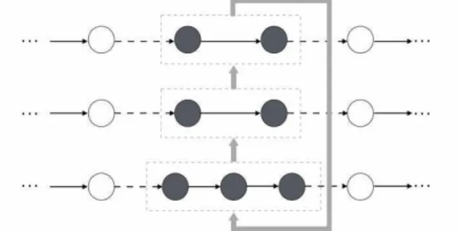
example of a cyclic-exchange operator with three routes is shown in Figure 2. The move-neighborhood operator can be regarded as a special form of cyclic-exchange operator. This operator moves the vertex sequence from one route to another, while no vertex is relocated from the second route.

Fig. 2. Graphical illustration of a cyclic-exchange move

operator is guided by the generalized objective function of the solution fAVNS( )S , instead of the construction cost in the generation of the initial solution. Each station h _{in the} reachable set of the route segment Η(L_j) is sorted in

ascending order of the objective function value of the resulting solution fAVNS(S←h), in which station is inserted.

The station indexed as 2

2 |H L( j) |

ρ

ϖ

⎢ ⎥

⎣ ⎦ is then selected,

where ϖ_{2 and}

2

ρ are defined the same as ϖ_{1 and}

1

ρ , respectively. After the selected station is located, the feasibility state of the route is updated. For the selected route, station-reconstruct repeats the preceding steps until the route becomes feasible in terms of battery driving limitation.

Fig. 3. Graphical illustration of the neighboring station set

Station-relocate replaces a current station with an un-located one in its neighboring station set. The neighboring station set of a located station is the set of stations that can replace the located one without affecting the feasibility of the solution regarding battery capacity. We provide a simple example in Figure 3 to better illustrate the neighboring set. The neighboring station set of the located station A can be determined as follows: Station A is removed from the route, and the separated vertices, v₂ and v3, are directly connected.

The first breaking vertex in the resulting route, which is vertex v₄, is found. The route segment before the first breaking vertex after the depot or a preceding station, which is { , , }v v_{1 2} v₃ , is identified, and the reachable set of the segment, which is { , , , , , , }A B C D E F G , is determined. The neighboring station of station A is the reachable set of the route segment excluding itself, that is,

( ) { , , , , , }

N A ₌ B C D E F G _{. The neighboring set can further}

be divided into two sets N_open( )A and N_unopen( )A based on

whether or not the stations in the neighboring set are located. After obtaining un-located stations in the neighboring set

( )

unopen

N A , the station-relocate operator ranks the stations in

the set N_unopen( )A in ascending order of objective function

value of the resulting solution fAVNS( ')S and replaces the

station with the one indexed by 3

3 |Nunopen( ) |w

ρ

ϖ

⎢ ⎥

⎣ ⎦, where

3 ϖ _and

3

ρ are defined the same as ϖ_{1 and} 1

ρ , respectively. The station-exchange operator substitutes the current station with a located one in its neighboring station set, and the implementation is the same as in the station-relocate operator, but with set N_open( )A .

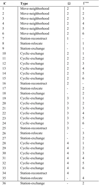
Table 1 presents the neighborhood structures based on the five operators within the shaking step of AVNS. The first nine structures consist of six move-neighborhoods, followed by one station-reconstruct, one station-relocate,

and one station-exchange. The three sets of neighborhood structures that comprise six cyclic-exchanges, one station-reconstruct, one station-relocate, and one station-exchange are presented from rows 10 to 18, 19 to 27, and 28 to 36. The number of routes involved Ω is not relevant for station-relocate and station-exchange but stands for the involved routes in station-reconstruct. The maximum length to exchange max

Γ in station-relocate and station-exchange represents the maximum number of charging stations to be relocated or exchanged, but it is irrelevant to station-reconstruct. Other rules of _Ω and max

Γ are also applicable to problem-specific operators.

4.4.2 Adaptive shaking

The AVNS in this work applies selection approaches in biasing the route, vertex sequence, and station selection involved in the shaking step to find promising solutions. The located station selection methods are newly designed for the problem, and the route and vertex sequence selection methods are similar to those in the VRPIS studied by Schneider et al. [29].

Route selection methods: Five selection methods are adopted to determine the first route in the subset of Ω routes that is involved in cyclic-exchange and station-reconstruct. The selection is performed in an iterative way;

Table 1. Parameters of the four real-world networks

κ

Type Ω max

Γ

1 Move-neighborhood 2 1 2 Move-neighborhood 2 2 3 Move-neighborhood 2 3 4 Move-neighborhood 2 4 5 Move-neighborhood 2 5 6 Move-neighborhood 2 6 7 Station-reconstruct 1 - 8 Station-relocate - 1 9 Station-exchange - 1 10 Cyclic-exchange 2 1 11 Cyclic-exchange 2 2 12 Cyclic-exchange 2 3 13 Cyclic-exchange 2 4 14 Cyclic-exchange 2 5 15 Cyclic-exchange 2 6 16 Station-reconstruct 2 - 17 Station-relocate - 2 18 Station-exchange - 2 19 Cyclic-exchange 3 1 20 Cyclic-exchange 3 2 21 Cyclic-exchange 3 3 22 Cyclic-exchange 3 4 23 Cyclic-exchange 3 5 24 Cyclic-exchange 3 6 25 Station-reconstruct 3 - 26 Station-relocate - 3 27 Station-exchange - 2 28 Cyclic-exchange 4 1 29 Cyclic-exchange 4 2 30 Cyclic-exchange 4 3 31 Cyclic-exchange 4 4 32 Cyclic-exchange 4 5 33 Cyclic-exchange 4 6 34 Station-reconstruct 4

that is, after selecting the first route, the remaining routes are iteratively selected from the routes that are spatially closer than a predefined threshold to the recently selected route. If no route is available in the confined area, the next route is to be randomly selected among all the routes. The selection mechanisms adopted to determine the first route are as follows:

1) Random: The probability of selecting each route has no difference.

2) Route length: The probability of selecting each route is proportional to the total length of the route.

3) Route length per demand unit: The probability of selecting each route is proportional to the ratio between total length and total demand.

4) Station density: The probability of selecting each route is proportional to the ratio of the number of stations to the number of total customers on the route.

5) Station detour: The probability of selecting each route is proportional to the total detour caused by the charging station of the route.

Vertex sequence selection methods: After the routes involved in cyclic-exchange are selected, the vertex sequence in each route is determined according to the following three mechanisms:

1) Random: The probability of selecting each vertex sequence has no difference.

2) Distance to the next route: The probability of selecting each vertex sequence is inversely proportional to the distance from the sequence to the route where it is going to be inserted. The distance is measured by summing up the distance of each vertex in the sequence to the center of the target route.

3) Distance to the neighboring vertex sequence: The probability of selecting each vertex sequence is proportional to the distance of the sequence to its surrounding vertices. The distance is calculated as the sum of the distance between the first vertex and its predecessor and that between the last vertex and its successor.

Station selection methods: Four selection approaches are proposed to select the located station. In particular, methods 1, 2, and 3 are used to select the to-be-replaced stations in the station-relocate operator, and methods 1, 2, and 4 are used to determine the stations in the station-exchange operator.

1) Random: The probability of selecting each station has no difference.

2) Number of related routes: The probability of selecting each station is proportional to the number of routes in the station services.

3) Number of neighboring un-located stations. The probability of selecting each station is proportional to the number of un-located stations in the neighboring station set.

4) Number of neighboring located stations. The probability of selecting each station is proportional to the number of located stations in the neighboring station set.

4.4.3 Adaptive mechanism

Given that the performance of each selection method differs across different problems, we apply the roulette wheel selection method to bias the selection of these methods based on probabilities [35]. As in ALNS, an adaptive mechanism is utilized in AVNS to assess the importance of selection methods by updating their probabilities. Considering a total of s selection methods, i₌1, 2,...,s,

each method is associated with a weight ωi , and the

probability of selecting the method i is given by

1

s

i j j

ω

ω

=

∑

. The weight of each selection method ωi is initialized with an equal weight at the beginning and updated every

η

AVNS AVNS iteration based on its performance. The performance of each method is measured by a scoring system, which assigns a score of nine to the method when a new overall best solution is found by the method, a score of three when the current solution is improved, and a score of one when the solution is worse than the current solution but is accepted by the acceptance criterion. Given the current score of method i, denoted by si, and the number of times it has been selected since the last weight update, denoted by

i

z , the new weight is then recalculated as

(1 ) ( )

i adp adp s zi i

ω

⋅ −

ρ

+

ρ

⋅ .

ρ

adp∈[0,1] is a parameter that controls the adaptive behavior, and si, zi are reset to zero after each weight update.

4.5 Tabu search component

The TS algorithm is applied to improve the routing plans in the solution S' _{generated from the AVNS phase. In every}

iteration, four operators are executed on the arc in the list of generator arcs to develop the neighborhood of the TS. The four operators are composed of three well-known operators, 2-opt*, relocate, exchange, and one problem-specific operator, StationInRe [22,36,37] . As is commonly done in the content of VRP, the TS algorithm regards a move as superior if the move can reduce the number of employed vehicles or has a better function value calculated with Eq. (42). In detail, the 2-opt* operator modifies the famous 2-opt to avoid the reversal of route directions. This operator is implemented for inter-route moves and allows the removal and insertion of the arc that includes a station visit. The relocate operator removes one vertex and inserts it into a different position on the same route or another route. The exchange operator switches the positions of the two vertices. Both relocate and exchange are applied for intra- and inter-route moves. However, the swapping of a station with a customer or another station is defined only for relocate. StationReIn is introduced to solve E-VRPTW, and it performs insertion and removals of charging stations.

The TS algorithm forbids the reinsertion of an arc into specific parts of the solution for a predefined number of iterations denoted by ς, which is randomly drawn from

min max

[

ς

,

ς

]

. Given that a visit to a station has a great effect on the battery level and time window obedience, a tabu attribute characterized by four elements

( , , , )

ι

k v w

is defined to prevent violations caused by reinsertion. The tabu attribute is used to prevent arc ι _{from being inserted into}

route rk between v and w , where v and w denote stations or depot. Through this process, an arc can be reinserted into a different part of the route. During the procedure, if a feasible new best solution is found, then the tabu status of a move is favored. After the predefined number of iteration

η

TS, the TS process is terminated. The

best solution found during TS is stored in solution S_'' as output.

4.6 Improvement procedure

an improvement procedure [6]. For all the located stations in each route rk , the procedure first selects the charging

stations in order and then removes the station from the route. If the removal of a station results in a battery capacity violation, the route is then split at the point with the least cost value. The cost value is calculated by

*

, ' , 1 , 1 , ' , 1 , 1

( ) ( )

r

e i o o i i i d i o o i i i

c

ε

d d d c t t t

+ + + +

⋅ ⋅ ₊ − ₊ ⋅ ₊ − , where

i denotes the split point, o o, ' the instances of depot, and

*

r e

c the electricity price in depot. The procedure ends when the number of vehicles approaches the maximum limitation or the solution cannot be improved any further. The solution produced, denoted by S_''', is compared with the current best solution S and evaluated by the acceptance mechanism illustrated below. If the solution S_''' is accepted, then S_''' replaces S, and

_κ

is reset to 1.

4.7 Acceptance mechanism

Aside from always favoring an improving solution, the AVNS/TS algorithm also accepts a new deteriorating solution if it passes the acceptance criterion [38]. The acceptance criterion is developed based on SA and allows the unsatisfying solution to be a new–current solution with a

certain probability

_e

−(fAVNS( ''')S −fAVNS( ))/S T_{. The value of the} probability is based on the difference between the new and current solutions, that is,

f

AVNS

( ''')

S

−

f

AVNS

( )

S

, and

temperature T . Temperature T is initialized with T0 and

updated using

T

n

=

ϑ

⋅

T

n−₁ after each iteration. If no

improving solution emerges in a predefined number of iterations denoted by

η

non, then the current solution is reset

to the best solution found so far. The value of T is set to T0

after

η

reset solution resets to diversify the solution.

5 Experimental studies

The performance of AVNS/TS on different sizes of instances is explored in terms of solution quality and computation time in this section. First, the parameter tuning is illustrated in Section 5.1, followed by the generation of instances in Section 5.2. Subsequently, the solution quality and effectiveness of the AVNS/TS algorithm are assessed with small- and large-scale instances in Section 5.3.

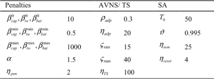
5.1 Experimental environment and parameter setting The experiments are conducted on a desktop computer with an Inter Core i5 processor at 2.67 GHz, with 4 GB of RAM and Windows 7 Professional. The AVNS/TS algorithm is implemented as a single-thread code in Java. Ten reasonably large instances are randomly generated to tune the parameters. The initial values of the parameters found during the development of our algorithm are input as basis for the tuning. One parameter is adjusted, while the others are kept

Table 2 summarizes the parameter settings for the initial penalty factors 0 0 0

, , cap tw bat

β β β , the bounds min min min

, ,

cap tw bat

β β β and

max max max

, ,

cap tw bat

β β β , the penalty update factor α _{, and the} number of penalty update iterations η_pen. For the algorithm,

the number of iterations after which the probabilities are updated is η_adp. The parameter that weighs the old and new

scores in the adaptive mechanism is ρ_adp. The minimal and

maximum tabu tenures are ς_min and ςmax, respectively. The

number of TS iterations is ηTS. The initial temperature parameter value is T0. The cooling rate is ϑ. The number of iterations after which the current solution is reset to the global best solution is ηnon. The number of solution resets

after which the temperature parameter is reset is ηreset. fixed. The best value of each parameter is determined after 20 runs on the generated test instances.

Table 2. Parameters of the parameters in AVNS/TS

Penalties AVNS/ TS SA

0 0 0 , ,

cap tw bat

β β β 10 ρadp 0.3 T0 50

min min min

, ,

cap tw bat

β β β _0.5 ηadp 20 ϑ 0.995

max max max

, , cap tw bat

β β β ₁₀₀₀ ςmin 15 ηnon 25

α _1.5 ςmax 40 ηreset 4

pen

η ₂ ηTS 100

We set the maximal number of AVNS/TS iterations to 800

η= for instances with less than 100 customers and

1.5

800 / (0.01 C)

η

= ⋅ for instances with more customers to achieve a good trade-off between run time and solution quality.

5.2 Generation of test instances

The instances for EV-MCS-LRPTW are generated based on the instances introduced in the pollution-routing problem (PRP) research of Demir et al., which consist of nine sets of instances with different sizes [39]. Specifically, we referred to their instances for network, customer demand, time windows, vehicle capacity, and driver wages. The speed of the vehicle is set to 90 km/h, the maximum speed in their research, to guarantee that all instances have at least one feasible solution in terms of time windows. The battery capacity of the vehicle is set to 80 kWh, as in the work of Davis et al. [40].

assumed to be 25 ㎡, and that of BSS is assumed to be twice that figure because of the automated equipment [32]. For the cost of back-up batteries at BSS, an apportioned cost by travel distance, called battery replacement cost, is utilized, instead of the total cost [20]. The electricity price at SCS, FCS, and SFCS is assumed to be the weighted average of the price at the peak period (0.5 USD/kWh for 2 pm–8 pm) and the price at the mid-peak period (0.2 USD/kWh for 7 am–2 pm and 8 pm–10 pm), and that at the BSS and depot is the

price of the off-peak period, 0.15 USD/kWh [42]. Table 3 summarizes the data.

5.2 Experiments on EV-MCS-LRPTW instances

In the numerical tests, the performance of the algorithm is first assessed on small-scale instances by comparing its results with those of the CPLEX Solver 12.2, and then it is evaluated with large-scale instances.

Table 3. Data of EV-MCS-LRPTW instances

Description Value Description Value

Loading capacity 3650 Set-up cost of BSS ($) 500000

Speed (km/h) 90 Area of SCS, FCS, and SFCS (㎡) 25

Battery capacity (kWh) 80 Area of BSS (㎡) 50

Stated range (km) 161 Average rental cost ($/㎡/day) 2.19

Speed (km/h) 90 Station lifetime of SCS (years) 15

Charging rate at SCS (kWh/min) 0.12 Station lifetime of FCS (years) 15 Charging rate at FCS (kWh/min) 1.05 Station lifetime of SFCS (years) 10 Charging rate at SFCS (kWh/min) 4.00 Station lifetime of BSS (years) 20 Time of battery swap at BSS (min) 10 Battery replacement cost ($/km) 0.20

Set-up cost of SCS ($) 6600 Driver wages ($/h) 13.14

Set-up cost of FCS ($) 60500 Average electricity cost at SFCS, SCS, FCS ($/kWh) 0.32

Set-up cost of SFCS ($) 126500 Electricity cost at BSS and depot ($/kWh) 0.15

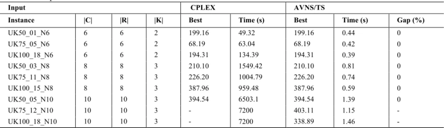
Table 4. Comparison of results obtained with CPLEX and AVNS/TS on the small-scale EV-MCS-LRPTW instances

Input CPLEX AVNS/TS

Instance |C| |R| |K| Best Time (s) Best Time (s) Gap (%)

UK50_01_N6 6 6 2 199.16 49.32 199.16 0.44 0

UK75_05_N6 6 6 2 68.19 63.04 68.19 0.42 0

UK100_18_N6 6 6 2 194.31 134.39 194.31 0.39 0

UK50_03_N8 8 8 3 210.10 1549.42 210.10 0.81 0

UK75_11_N8 8 8 3 226.20 1004.79 226.20 0.74 0

UK100_15_N8 8 8 3 387.96 959.48 387.96 0.59 0

UK50_05_N10 10 10 3 394.54 6503.1 394.54 1.39 0

UK75_12_N10 10 10 3 - 7200 403.11 1.15 -

UK100_18_N10 10 10 3 - 7200 338.89 1.46 -

Tab. 5. Results of results AVNS/TS on the large-scale EV-MCS-LRPTW instances

Input Result

Instance |C| |R| |K| SCS FCS SFCS BSS Best Time (min)

UK50_01 50 50 10 1 2 1 0 838.88 10.56

UK50_07 50 50 10 1 1 0 0 541.29 7.51

UK50_10 50 50 10 1 2 1 0 906.05 16.27

UK50_14 50 50 10 1 2 1 0 889.90 13.00

UK75_03 75 15 15 1 3 0 0 1020.01 21.53

UK75_05 75 15 16 1 2 1 0 1061.73 34.92

UK75_11 75 15 16 1 2 0 0 794.56 16.84

UK75_17 75 15 16 1 2 1 0 1084.41 30.56

UK100_07 100 20 19 1 3 1 0 1328.59 57.47

UK100_09 100 20 20 1 1 1 0 1055.17 48.90

UK100_12 100 20 19 1 2 1 0 1199.35 50.34

UK100_19 100 20 20 1 3 2 0 1598.84 71.22

UK150_01 150 30 30 1 2 1 0 1542.47 105.06

UK150_05 150 30 30 1 2 1 0 1587.59 107.30

UK150_13 150 30 29 1 3 0 0 1649.29 84.45

UK150_19 150 30 30 1 2 2 0 1941.96 146.07

UK200_07 200 40 40 1 2 1 0 2002.45 210.83

UK200_10 200 40 42 1 1 1 0 2037.46 171.25

UK200_16 200 40 40 1 2 1 0 2046.07 193.24

The quality and run time of AVNS/TS on small instances is tested using several instances. The instances are generated by randomly selecting C _{customers from the}

given instances. For example, UK50_01_N6 represents the instance in which six customers are selected from 50 customers in PRP instances. Both the AVNS/TS algorithm and the CPLEX solver are applied to solve the generated instances. The results are summarized in Table 4.

For clarity, columns 1 to 4 describe the basic structures of instances, where the number of customer number, candidate station sites, and vehicles are presented sequentially. The results and computing time are listed in columns 5 and 6, respectively. Columns 7 to 9 show the computational result of the AVNS/TS algorithm, computing time, and gap between the results using AVNS/TS and the CPLEX. As is commonly done, a time limit of 7,200s (2h) is set for all the instances. If the CPLEX solver fails to find the optimal solution for an instance, we use the symbol “-” to indicate its result. From the computing results, the AVNS/TS algorithm can effectively find the optimal solution.

Subsequently, the AVNS/TS is applied to solve large-scale instances. Table 5 presents the results of 20 instances with objective function values and computation times. In detail, columns 1 to 4 depict the feature of the instances. Columns 5 to 8 show the result of the charging station strategy. For each instance, the algorithm is executed five times, from which the best solution is recorded in column 9, and the related run time in minute is presented in column 10.

The computation results imply that AVNS/TS can solve large-scale instances within reasonable time. The optimal solutions of several instances indicate that multiple types of charging stations should be considered to reach the minimum cost. The results also imply that SCS, with a minimal construction cost among the four types of stations, is suitable for the central depot, which is reasonable from the cost perspective. Meanwhile, a combination of FCS and SFCS is more suitable in most cases. The BSS type is not selected for any of the 20 instances mostly because its

construction cost is much higher than those of FCS and SFCS.

6. Conclusions

This paper introduces EV-MCS-LRPTW, an extension of LRP, to optimize the routing of EVs and the strategy of charging stations under the constraints of loading capacity, battery capacity, and time windows. Contrary to existing research on EVs, this problem considers the possibility of using different types of charging infrastructure and optimizes the type selection of infrastructures along with the station location decision and routing plan. This problem is highly relevant in the context of EVs because charging stations are critical to EVs. The optimal selection of charging infrastructure can save money for logistic companies in the long run because each charging technology has its pros and cons in terms of charging speed, economic investment, and practical requirement.

We developed a hybrid heuristic that combines AVNS with the TS algorithm for intensification to address the problem. A number of instances with realistic data were designed to validate the algorithm in the experimental studies. The computational results indicate that the algorithm can effectively reach nearly optimal solutions for small-scale instances, in contrast to the CPLEX solver. The algorithm also provided convincing results in moderate run time for large-scale instances. The results on realistic-sized instances demonstrate that incorporating multiple types of charging infrastructure in the station strategy and routing plan can result in a better solution than considering a single charging infrastructure under the constraints of time windows.

In future, the problem can be extended to include multiple depots or consider a mixed fleet with EVs and ICVs. The existence of public charging stations can also be incorporated into the problem. The work can be extended by further considering specific characteristics of EVs.

Acknowledgements

This work was supported by the National Natural Science Foundation of China under the project No.71271137, and the Natural Science Foundation of Shanghai under the project No.12ZR1415100.

______________________________

References

1. Eggers, F., Eggers, F., “Where have all the flowers gone? forecasting green trends in the automobile industry with a choice-based conjoint adoption model”. Technological Forecasting & Social Change, 78(1), 2011, pp.51–62.

2. National Renewable Energy Laboratory, “Project Startup: Evaluating the Performance of Frito Lay’s Electric Delivery Trucks.” 2014. Web. 3 Dec. 2015. <http://www.nrel.gov/docs/fy14osti/61455.pdf>.

3. Heineken International “Case Studies: Europe’s Largest Electric Truck Will Drive down Emissions.” 2014. Web. 2 Dec. 2015. <http://sustainabilityreport.heineken.com/ Reducing-CO2- emissions/Case-studies/Europes-largest-electric-truck-will-drive-down-emissions/index.htm>.

4. DHL International, “Deutsche Post DHL Fleet of Alternative Vehicles Continues to Grow.” 2014. Web. 2 Dec. 2015. <http://www.dhl.com/en/press/releases/releases_2014/group/dp_dhl_fle et_of_alternative_vehicles_continues_to_grow.html>.

5. Wang, Y. W., Lin, C. C., “Locating multiple types of recharging stations for battery-powered electric vehicle transport”. Transportation Research Part E: Logistics & Transportation Review, 58, 2013, pp. 76-87.

6. Yang, J., Sun, H., “Battery swap station location-routing problem with capacitated electric vehicles”. Computers & Operations Research, 55, 2015, pp.217-232.

7. Schneider, M., Stenger, A., Goeke, D., “The electric vehicle-routing problem with time windows and recharging stations”. Transportation Science, 48(4), 2014, pp.500-520.

8. Nagy, G., Salhi, S., “Location-routing: Issues, models and methods”.