Nonlinear instability of baroclinic atmosphere with reference to planetary scale disturbances

(1)

SRef-ID: 1607-7946/npg/2004-11-363

Nonlinear Processes

in Geophysics

Nonlinear instability of baroclinic atmosphere with reference to

planetary scale disturbances

I. A. Pisnichenko

Center for Weather Forecasting and Climate Studies/Brazilian National Institute for Space Research, Brazil on leave from A. M. Obukhov Institute of Atmospheric Physics, Russian Academy of Sciences, Moscow, Russia Received: 27 May 2003 – Revised: 12 July 2004 – Accepted: 24 July 2004 – Published: 2 August 2004

Abstract. In this paper we investigate the stability of

zonal flow in a baroclinic atmosphere with respect to finite-amplitude planetary-scale disturbances by applying Arnold’s method. Specifically, we examine the sign of the second vari-ation of a conserved functional for the case of a polytropic at-mosphere (i.e. one with a linear lapse rate) and with a linear profile of zonal wind. Sufficient stability conditions for an infinite atmosphere (i.e. with a temperature lapse rate equal to zero) are satisfied only for an atmosphere in solid body rotation. For a polytropic atmosphere of finite extent (a lapse rate is not equal zero) the sufficient conditions of stability can be satisfied if a lid is placed below min(Zmax, polytropic

atmospheric height). The dependence of heightZmaxon

val-ues of the vertical gradient of the zonal wind and the zonal temperature distribution is calculated.

1 Introduction

Ultra-long atmospheric waves play a significant role in the formation of weather and climate regimes. The longest waves dominate the spectral distribution of kinetic and avail-able potential energy. The ultra-long waves are responsible for both energy transfer through the spectrum (Baines, 1976; Starr, 1968) and for heat transfer from the lowest layer of the troposphere to the stratosphere (Charney and Drazin, 1961; McNulty, 1976). The first three spherical harmonic compo-nents (ψ₁0, ψ₁1, ψ₁−1) are directly connected with the angular momentum of the Earth (Barnes et al, 1983; Pisnichenko, 1990). There is a large correlation between events of block-ing formation and the values of amplitudes and phases of stationary spherical harmonics withm =2,3 in the geopo-tential field (Kurbatkin, 1970; Bengtsson, 1981). Planetary waves are also responsible for low-frequency atmospheric variations and, as a consequence, for the manner of the tem-poral evolution of stochastic atmospheric regimes (James and Correspondence to:I. A. Pisnichenko

([email protected])

James, 1992; Kurgansky et al, 1996). For these reasons, investigation of peculiarities in the behaviour of ultra-long waves is important for undestanding of climate processes and for the construction of climate simulation models.

Some of the principal properties of ultra-long waves are related to the stability of the atmospheric zonal flow. The growth rates and the height distribution of the amplitudes of unstable ultra-long waves are central characteristics that, to a great extent, define the dynamics of the large-scale atmo-spheric circulation.

In Lynch (1979), the instability of zonal flow with respect to ultra-long waves was studied by means of linearised plan-etary geostrophic equations of type II. These equations de-scribing planetary-scale disturbances were first proposed by Burger (1958) and were later used in the works of Wiin-Nielsen (1961), Phillips (1963), Pisnichenko (1980, 1983), and others. Important insights into the dependence of the growth rate of ultra-long waves on the wind shear and the coefficient of static stability were obtained using this linear approach.

(2)

temperature fields. Section 4 is devoted to the calculation of first and second variations of a functional composed of con-servation integrals. The conditions of sign definiteness of the second variation define the sufficient conditions of zonal flow stability. The general equation obtained here are applied for the case of polytropic atmospheres in Sect. 5.

2 The model equations

We will consider three-dimensional baroclinic atmospheric flow of planetary scale on the spherical Earth. The equations used are the quasi-geostrophic equations of type II first de-rived by Burger (1958). For the dry adiabatic case they are written in the form:

f u= − 1

ρa ∂p

∂ϕ (1)

−f v = − 1

ρacosϕ ∂p

∂λ (2)

g = −1

ρ ∂p

∂z (3)

∂ρ

∂t + ∇ ·ρv = 0 (4)

ds

dt = 0 (5)

p = RρT (6)

whereu, v, ware the zonal, meridional and vertical compo-nents of velocity vectorv; p,ρ, ands are respectively the air pressure, density, and specific entropy of dry air with gas constantR;f =2ωsinϕis the Coriolis parameter;ωis the angular velocity of the Earth’s rotation;gis the gravitational acceleration force for unit mass; andλ, ϕ, zare longitude, latitude and height above the surface of a spherical Earth of radiusa. Differential operators of total derivatived/dt and divergence in spherical coordinates are

d dt =

∂ ∂t +

u acosϕ

∂ ∂λ +

v a

∂ ∂ϕ +w

∂ ∂z.

∇ ·v= + 1

acosϕ ∂u ∂λ+

1 acosϕ

∂

∂ϕ(cosϕ v)+ ∂w

∂z From equations (1 - 6), the following conservation laws can be obtained:

a) conservation of the planetary potential vorticity (trans-posed potential vorticity) of an air parcel (see Appendix for details)

d dt

f ∂s_∂z ρ =

d

dt =0; (7)

b) globally-integrated conservation of total potential energy d

dt

Z Z Z

V

ρ(gz+cvT ) dτ =

d5

dt =0; (8)

c) conservation of any globally-integrated mass-weighted function of potential vorticity and potential temperature

d dt

Z Z Z

V

ρ8(, s) dτ =dF

dt =0, (9)

where8is any function ofands;

d) conservation of transposed angular momentum (the angu-lar momentum of the atmosphere if it were in solid rotation with the earth)

d dt

Z Z Z

V

ωa2cos2ϕρ dτ= dM

dt =0. (10) e) conservation of any surface-integratedf-weighted func-tion of entropy

d dt

Z Z

S

f G(s) dσ= dP

dt =0, (11)

whereGis an arbitrary function of specific entropy and the integral is calculated over the plane Earth’s surface (wshould be equal to zero at the Earth’s surface).

3 Bernoulli’s theorem

We will investigate the stability of atmospheric zonal flow according to the scheme described by Dikiy (1965) and Dikiy and Kurgansky (1971). We begin by showing that a steady flow (∂/∂t=0) described by Eqs. (1–6) satisfies Bernoulli’s theorem. To prove this, multiply Eqs. (1), (2), and (3) by a dϕ,acosϕ dλanddz, respectively, and add. We obtain: f (u a dϕ−v acosϕ dλ)+g dz= −1

ρdp. (12) For a streamline,

acosϕ dλ

u =

a dϕ v =

dz w,

so the parenthetical term in Eq. (12) drops out along a stream-line, leaving Bernoulli’s theorem:

d gz= −1

ρdp. (13)

Next we show thatds = 0 along a streamline. For this, multiply Eq. (5) for steady flow bydt and note thatu dt =

acosϕ dλ,vdt=a dϕ, andwdt =dz. Then, using the first law of thermodynamics, we obtaind(gz+cpT )=0 or

gz+cpT =const

along a streamline.

(3)

4 A conserved functional and its first and second varia-tions

To investigate the stability of a zonal flow let us compose the functional from the integrals of motion (Eqs. 8—11). This procedure is to some extent similar to finding conditional ex-tremum of a function with the help of a Lagrange multiplier. The integrals of motion that we use here correspond to con-straints that set some limitations on possible motions. H=5+F +P +qM=

Z Z Z

V

ρ[gz+cvT +8(s, )+

+qωa2cos2ϕidτ+ Z Z

S

f G(s) dσ. (14) The temperatureT in functionalH can be expressed in terms of specific entropy asT = T∗exp(s/cv)(ρ/ρ0)κ−1

whereκ =cp/cvandT∗is a constant having the dimension

of temperature. Symbolq corresponds here to any arbitrary constant. Denoting the value of the functionalH correspond-ing to the zonal flow under discussion asH0and expanding

the functionalH in a Taylor series in the vicinity ofH0we

write:

H=H0+δH|H0 +δ 2_H_|

H0+. . . .

If the first functional variationδH|H0 is equal to zero, then the zonal flow corresponding to the functional valueH0is a

stationary point in the functional{, s}-space. Performing the calculation we will obtain the following expression for the first variation ofH:

δH= Z Z Z

V

h

9+8−8+qωa2cos2ϕ

δρ

+ρ

T +8s−8s−8

f ρ

∂ ∂z

δs

dτ

+ Z Z

S

f (Gs−8) δs dσ. (15)

One can see from Eq. (15) that necessary conditions for δH=0 are the following

9+8−8+qωa2cos2ϕ=0 (16)

8s−8s−8

f ρ

∂

∂z +T =0 (17) G′(s)−8|z=0=0 (18)

Note here that Eq. (17) is a consequence of Eq. (16). To prove this, it suffices to differentiate Eq. (16) with respect to zand then to divide the result obtained by∂s/∂z 6= 0. If arbitrary functions8andGare chosen to satisfy Eqs. (16) and (18) then for our zonal flowH0will be a stationary point.

For the second variation ofHwe will have:

δ2H = Z Z Z

V

_(κ₋

1)cpT

ρ (δρ)

2₊_2(κT ₋₈

s

+8s)δρδs+ρ8(δ)2+ρ

8ss+

T cv

−8ss

−8s

f ρ

∂ ∂z

(δs)2

dτ+ Z Z

S

(Gss−8s) f (δs)2dσ.(19)

Here we designateδ=f/ρ δ(∂s/∂z) −f/ρ2∂s/∂zδρ, and 8,8s, . . . as partial derivatives of function8with

respect to,s.

Differentiating Eq. (17) with respect toz, we find:

8ss−8ss−8s

f ρ

∂ ∂z =

1 sz

_∂

∂z(8 f ρ

∂ ∂z)−Tz

,(20)

and finally differentiating Eq. (16) with respect toφand tak-ing into account Eq. (17), we obtain:

8=

ρ(qωa2sin 2ϕ+T ∂s_∂ϕ −cp∂T_∂ϕ)

(s, )af . (21) Here(s, )=(∂s/∂ϕ ∂/∂z − ∂/∂ϕ∂s/∂z)/a.

Using Eqs. (17), (20), (21) we can rewrite the second vari-ation ofHas:

δ2H = Z Z Z

V

₁

ρ(κ−1)cpT (δρ)

2₊

2

(κ−1)T +

_∂

∂z

·f u+qωasin 2ϕ

(s, )

δρδs+ρ

2_{(f u}₊_qωa_{sin 2ϕ)}

f (s, ) (δ)

2₊

ρ

_T

cv

+ 1

sz

_∂

∂z

_∂

∂z

f u+qωasin 2ϕ (s, )

−Tz

(δs)2

dτ

+ Z Z

S

ρϕ sϕ

(f u+qωasin 2ϕ) (s, ) (δs)

2_dσ.

(22)

The surface integral expression was obtained by differentiat-ing Eq. (18) with respect toϕ. We also have used here the alternative form of Eq. (1)

f u= −cp

a ∂T ∂ϕ +

T a

∂s

∂ϕ. (23)

Note thatδ2Hrepresents a functional from two independent functions becausecan be expressed throughρands.

If we consider zonal flow with δH = 0, and if δ2H is sign-definite at a certain point in functional space of two in-dependent functions, then this point will be a maximum (or minimum) of functionalH in this functional space. Level functional surfaces in functional space around this point will be closed and inserted one into another. Thus, in the case of a finite disturbance of the zonal flow, the phase point cor-responding to the new disturbed state will shift to one of these surfaces and will stay on it, asdH /dt = 0. During all next time, the phase point will not strongly deviate from the extremum point corresponding to the initial zonal flow (Arnol’d, 1965).

5 The case of a polytropic atmosphere

Let us now consider a polytropic atmosphere (T =T0−γ z).

We will assume that the wind changes linearly with a height: V = V0+3z, as is frequently used in zonal flow stability

(4)

For further calculations it is convenient to express terms entering the functional (22) through3,γ,T,ρ.

δ2H= Z Z Z

V      1 ρ  

(κ−1)cpT−

κ2g(f u+qωasin 2ϕ(γa−γ )

_{f 3κ}

κ−1+

βg(γa−γ )

f γa

γa   (δρ) 2₊ +2  

(κ−1)T−

g(f u+qωasin 2ϕ)(γa+κ(κ−1)(γa−γ ))

_{f 3κ}

κ−1+

βg(γa−γ )

f γa

Rγa



 δρδs+

+ρ    T cv

+ T γ

cp(γa−γ )

− f T 3γa

f 3κ κ−1+

βg(γa−γ )

f γa

R(γa−γ )

−

−g(f u+qωasin 2ϕ)(γa−γ )

f 3κ κ−1+

βg(γa−γ )

f γa

c2

vγa

  (δs) 2      dτ+ + Z Z S

(f2u0+RT β)(f u0+qωasin 2ϕ)ρ0γa

(u_T0

0−

3 γa−γ )(

f 3κ κ−1+

βg(γa−γ )

f γa )(γa−γ )Rf

2

(δs)2dσ.(24)

Here we designate∂f/a∂ϕ=βand have used the following equation:

∂s ∂z=

(γa−γ )cp

T ; =

f (γa−γ )cp

ρT ; z=

g RT; ∂s a∂ϕ = _{f u} T − f 3 γa−γ

_γ

a−γ

γa ; ∂ a∂ϕ = T _{f u} R + T β f

; δ= −

cvρ

(ρδs+cpδρ);

(s, )= −

T

_{f 3κ}

κ−1 +

βg(γa−γ )

f γa

.

Letu0= −qacosϕ. This means that the wind on the Earth’s

surface represents solid body rotation. The intensity and di-rection of the wind is defined by the arbitrary parameterq. In this case, the surface integral in Eq. (24) is zero, and the suffi-cient conditions required for the volume integral part ofδ2H to be sign-definite quadratic form, are also sufficient condi-tions for stability of the zonal flow with respect to planetary scale disturbances.

The second variationδ2Hwill be sign-definite if: 1

ρ





(κ−1)cpT −

κ2g(f u+qωasin 2ϕ)(γa−γ )

(_κf 3κ₋ 1 +

βg(γa−γ )

f γa )γa

   ·ρ _T cv

+ T γ

cp(γa−γ )

−

− f T 3γa

(f 3κ κ−1+

βg(γa−γ )

f γa )(γa−γ )R

−g(f u+qωasin 2ϕ)(γa−γ )

(f 3κ κ−1+

βg(γa−γ )

f γa )c

2

vγa

   −  

(κ−1)T−

g(f u+qωasin 2ϕ)(γa+κ(κ−1)(γa−γ ))

(f 3κ κ−1+

βg(γa−γ )

f γa )Rγa



  2

>0.(25)

Substituting values forT =T0−γ zand foru= u0+3z

we can rewrite it as

_{κf 3}

κ−1+

βg(γa−γ )

f γa

−2 ·

(

z2

"

(κ−1)β2g2γ2(γa−γ )

f2_γ

a

+κ(3−κ)3βgγ2 +

+2κ2f232γaγ−κ(2−κ)3βgγaγ−

κ3f232γ_a2 κ−1

2+ 1

κ(κ−1)

# +

+zT0 "

2κ2f232γa

κ−1 +κ(2−κ)3βgγa−κ(4−κ)3βgγ +

+2(κ−1)β 2_g2_{γ (γ}

a−γ )

f2_γ

a

# +

+κT₀23βg+(κ−1)T 2 0β

2_g2_(γ

a−γ )

f2_γ

a

)

>0. (26)

For an atmosphere of any vertical extent this inequality will be satisfied everywhere only when3 = 0, (because at the pole the term in rectangular parenthesis atz2will be neg-ative for any3), that is, when the whole atmosphere rotates as a solid body (note thatu0= −qacosϕ).

For the case of isothermal stratification Eq. (26) will take the form

_{κf 3}

κ−1+ βg f −2 · ( −κ

2_f2₃2_γ2

a[(κ−1)2+κ2]

(κ−1)2 z 2₊_κT

03γa ·

"

2f2κ3

(κ−1)+(2−κ)βg

#

z+

+κT₀23βg+(κ−1)T 2 0β

2_g2

f2 )

>0. (27)

Hence it follows that Eq. (27) is satisfied everywhere only for the trivial case of3 = 0. The quadratic formδ2H for an isothermal atmosphere will be sign-indefinite for an at-mosphere of any vertical extent, when

g2T232 c2

v

[βg(2−κ)+2f 2_κ3

(κ−1)]

2₊

+4f

2_g2₃2_[_(κ₋₁₎2₊_κ2_]

c2

v(κ−1)2

[g 2

f2(κ−1)T

2_β2₊_κβgT2₃_]_<

(5)

0.0 0.003

0.006

0.009

-0.004 -0.002 0 0.002 0.004

zonal wind vertical gradient, 1/s

0 10 20 30 40 50 60 70 80 90

lat, degrees

Fig. 1. The areas of stability for a finite atmosphere are located to the right of the curves. The curves marked from top to bottom

correspond to lapse rates ofγ = 0 K/m, 0.003 K/m, 0.006 K/m,

0.009 K/m.

On the other hand, the quadratic formδ2H can be sign-definite for an atmosphere of finite height. For this, it is nec-essary that one of the roots of Eq. (26) be positive and the other be non-positive, and a lid has to be placed at a height that is equal to or less then the positive root value. Hence the δ2H will be sign-definite for a finite isothermal atmosphere if

3 >−gβ(κ−1)

f2_κ

and the atmosphere is capped by a lid at positive heightZ0≤

Zmaxwhere

Zmax=

Tβg(2_κ−κ)+2_κf₋23₁ + q

β2_g2_(κ₊₃₎

κ−1 +

4f2_βg(κ2₊_κ₋₁₎₃

κ(κ−1)2 + 4f4₃2

(κ−1)2

2f2_γa3_[_(κ₋₁₎2₊_κ2_]

(κ−1)2

.(28)

Because the zonal velocity changes quasi-linearly with height in free atmosphere, it can be expected that velopause position will be close toZmax. In Fig. 1, the area of

stabil-ity corresponding to isothermal stratification is situated to the right of the curve marked as 0.0.

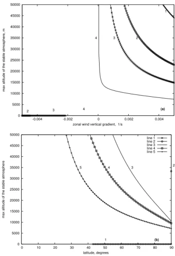
Figure 2 shows the dependence ofZmax onϕ and3for

isothermal stratification when3=const in the whole atmo-sphere, andT is expressed using the thermal wind equation asT =TeqeDcosϕ. Here the following designation are used:

D=2ω3/g,Teqis a surface temperature on the equator.

Figure 3 presents the dependence ofZmaxon latitude,ϕ,

and the equator-to-pole temperature contrast, 1T. Specif-ically, we model the surface temperature as T = Tp +

1Tcosϕ, where Tp is the surface temperature at the pole

and1T =Teq−Tp.

In the general case of a polytropic finite atmosphere, the area of stability decreases with increasing lapse rateγ (Fig. 1). In the model used,γ does not depend on latitude

0 5000 10000 15000 20000 25000 30000 35000 40000 45000 50000

-0.004 -0.002 0 0.002 0.004

max altitude of the stable atmosphere, m

1

2 3 4

4 (a) 3

2

0 5000 10000 15000 20000 25000 30000 35000 40000 45000 50000

0 10 20 30 40 50 60 70 80 90

max altitude of the stable atmosphere

latitude, degrees

5 4 3

1 (b) 2 line 1 line 2 line 3 line 4 line 5

Fig. 2.Dependence ofZmaxin a vertically isothermal atmosphere

(γ = 0) on the zonal wind vertical gradient3(a)and latitudeϕ

(b)for the case when3is constant in the whole atmosphere. In

(a), curves 1–4 correspond to latitudes 30◦, 45◦, 60◦, and 90◦. In

(b), curves 1–5 correspond to3= −0.005 s−1, 0 s−1, 0.001 s−1,

0.002 s−1, and 0.005 s−1.

ϕ. To show this, it suffices to differentiate the momentum equation (23) with respect toz:

f cp

∂u ∂z = −

cp

a ∂2T ∂z∂ϕ +

T a

∂2s ∂z∂ϕ +

1 a

∂s ∂ϕ

∂T

∂z (29)

Using Eq. (23) and the thermal wind equation f 3 = −γf u

T − cpγa

T a ∂T ∂ϕ

one can express the meridional gradient of entropy as 1

a ∂s ∂ϕ =

_{f u}

T − f 3 γa−γ

_γ

a−γ

γa

.

Substituting this result into Eq. (29) we conclude that ∂2T /∂z∂ϕ=∂γ /∂ϕ=0.

The maximum height of a polytropic stable finite atmo-sphere model is min(T0/γ , Zmax). Zmax for this case

(6)

0

5000 (a) 10000

15000 20000 25000 30000 35000 40000 45000 50000

25 30 35 40 45 50 55

equator-pole temperature difference, K 1

2

3

4

0

5000 (b) 10000

15000 20000 25000 30000 35000 40000 45000 50000

0 10 20 30 40 50 60 70 80 90

latitude, degrees 4 3 2 1

Fig. 3. Dependence ofZmaxon the equator-to-pole temperature

contrast,1T (a), and on latitude,ϕ(b). The meridional surface

temperature distribution is modelled asT = Tp+1Tcosϕ, and

vertical temperature gradient is constant (γ=0). In (a), curves 1–4

correspond to latitudes 45◦, 60◦, 75◦, and 90◦. In (b), curves 1–3

correspond to1T =25 K, 35 K, 45 K, and 55 K.

dependence ofZmax on these parameters is presented.

Re-sults depend weakly onα. Here the calculations were made for α = 5m/s. For the calculations with3 which do not depend on latitude, to satisfy the thermal wind equation we modelled surface temperature for the flow of interest asT0=

Teqexp{B(cosϕ−1)}+2A/B2(1+B)exp{B(cosϕ−1)}−

2A/B2(1 + Bcosϕ), where A = γ ωα/ag, and B =

2ω3a/g.

In these figures one can see that the rate of the change ofZmax with latitude noticeably depends both on3andγ

(Fig. 4). However the minimum height ofZmax on a pole

does not strongly vary and is equal to approximately 8-9 km (Fig. 5b). The dependence ofZmaxon the pole-equator

tem-perature difference1T, latitudeϕ and temperature gradient γ shows that the area of stability strongly diminishes under the approximationγ equalsγa(Fig. 6a).

0

5000 (a) 10000

15000 20000 25000 30000 35000 40000 45000 50000

0 10 20 30 40 50 60 70 80 90

latitude, degrees

1 5 4 3 2

0

5000 (b) 10000

15000 20000 25000 30000 35000 40000 45000 50000

0 10 20 30 40 50 60 70 80 90

latitude, degrees

1 5 4 3 2

0

5000 (c) 10000

15000 20000 25000 30000 35000 40000 45000 50000

0 10 20 30 40 50 60 70 80 90

latitude, degrees

1 5 4 3 2

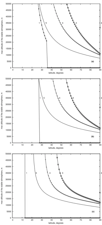
Fig. 4. Dependence of the maximum heightZmaxof a finite

sta-ble atmosphere on latitudeϕfor three values ofγ: 0.003K/m- in

(a), 0.006K/m- in(b), and 0.009K/m-(c). The curves labelled

1–5 correspond to constant values of 3 = −0.005s−1, 0 s−1,

0.001 s−1, 0.002 s−1, and 0.005 s−1.

6 Discussion and conclusions

(7)

0

5000 (a) 10000

15000 20000 25000 30000 35000 40000 45000 50000

-0.004 -0.002 0 0.002 0.004

zonal wind vertical gradient, 1/s 1

1 2

2 3

3

0

5000 (b) 10000

15000 20000 25000 30000 35000 40000 45000 50000

-0.004 -0.002 0 0.002 0.004

1

2

3

3 4

4

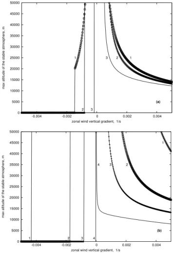
Fig. 5. Dependence of the maximum height of a finite stable

at-mosphereZmaxon the zonal wind vertical gradient3. In(a)for

latitudeϕ=60◦the curves marked by numbers correspond to: ’1’

toγ = 0.003K/m, ’2’ -γ = 0.006K/m, ’3’ -γ = 0.009K/m;

on(b)for the stratification withγ =0.006K/mthe curves marked

by numbers corresponding: ’1’ toϕ = 30o, ’2’ -ϕ = 45◦, ’3’

-ϕ=60◦, ’4’ -ϕ=90◦. The calculations correspond to the case of

3=const.

For the case of surface wind in solid body rotation, the sta-bility of the zonal flow depends on the sign-definiteness only of that part the second variation of a functional which is rep-resented by the three-dimensional integral. Zonal flow stabil-ity was examined directly for the case when the zonal wind changes linearly with height in a polytropic atmosphere.

In an isothermal atmosphere of infinite height, the zonal flow is stable only if the whole atmosphere rotates as a solid body. In an atmosphere bounded by an upper lid, the zonal flow can be stable when vertical shear in zonal wind exists.

For a negative value of the zonal wind vertical gradient (∂V /∂z <0), that is, when surface air temperatures increase from equator to pole, the atmosphere is always unstable. For a positive value of∂V /∂z, stability depends on the height at which the lid is placed. The height of the lid in turn depends on∂V /∂zand latitude, and decreases when∂V /∂zand lati-tude increase. For stability, the minimum height at which the lid would have to be placed at the pole is 8–9 km for the case of the observed values of vertical shear.

0

5000 (a) 10000

15000 20000 25000 30000 35000 40000 45000 50000

25 30 35 40 45 50 55

equator-pole temperature difference, K

1a

1b

1c 2a

2b

2c

3c, 3b, 3a

0

5000 (b) 10000

15000 20000 25000 30000 35000 40000 45000 50000

0 10 20 30 40 50 60 70 80 90

latitude, degrees

1 2 3

Fig. 6. Dependence ofZmaxon 1T (a)andϕ (b) for the case

where the meridional surface temperature distribution is described

asT =Tp+1Tcosϕ. In (a) the curves marked as ’1a’, ’1b’, ’1c’

correspond to latitudes 45◦, 60◦, 90◦andγ = 0.003 K/m; ’2a’,

’2b’, ’2c’ correspond to the same latitude andγ = 0.006 K/m;

and ’3a’, ’3b’, ’3c’ correspond to the same latitude andγ =0.009

K/m. In (b)γ = 0.006 K/m, and curves ’1 –3’ corresponds to

1T =25 K, 40 K, and 55 K.

As expected, the area of stability in latitude and∂V /∂z parameter space decreases as the vertical temperature gradi-entγ increases. For an adiabatic lapse rate, the zonal flow can become unstable for all values of∂V /∂z, even in a finite atmosphere. The area of instability appears near the equator and extends to the poles with increasingγ.

Appendix

To prove Eq. (7) it is necessary to apply to Eq. (1) an operator ∂/acosϕ∂λand to Eq. (2) an operator−∂/a∂ϕand to add. As a result we obtain (expressingpandρ throughsandT from ideal gas entropy equation)

df dt +

f acosϕ

_∂u

∂λ+

∂(v cosϕ) ∂ϕ

=

1 a2_cosϕρ2

_∂T

∂λ ∂s ∂ϕ −

∂T ∂ϕ

∂s ∂λ

(8)

Differentiating the entropy conservation Eq. (5) with re-spect toz, we have

d dt

_∂s

∂z

+ 1

acosϕ ∂s ∂λ

∂u ∂z +

∂s a∂ϕ

∂v ∂z +

∂s ∂z

∂w

∂z. (31) Then using equations for thermal wind

f∂u ∂z =

∂T ∂z

∂s a∂ϕ −

∂T a∂ϕ

∂s ∂z f∂v

∂z = − 1 a cosϕ

∂T ∂z

∂s ∂λ+

1 a cosϕ

∂T ∂λ

∂s ∂z and equation for vertical gradient of entropy

∂s ∂z=

cp

T

_g

cp

+∂T

∂z

and adding Eq. (30) divided byf and Eq. (31) divided by ∂s/∂zand subtracting the continuity Eq. (4) divided byρwe come to the equation

d dt

f ∂s_∂z ρ =0.

Acknowledgements. The financial support for this research by the Brazilian National Council for Development of Science and

Technology (CNPq) is gratefully acknowledged. I want also

to thank M. V. Kurgansky and S. Nilo Figueroa for the useful discussions.

Edited by: A. Osborne Reviewed by: two referees

References

Arnol’d, V. I.: On the conditions for nonlinear stability of stationary plane curvilinear flows of an ideal fluid (in Russian), Dokl. Akad. Nauk SSSR, 162, 975–978, 1965, (English transl.: Sov. Math., 6, 773–777, 1965.)

Baines, P. G.: The stability of planetary waves on a sphere. J. Fluid Mech, 73, 2, 193–214, 1976.

Barnes, R. T. H., Hide, R., F. R. S., White, A. A., and Wilson, C. A.: Atmospheric angular momentum fluctuations, length-of-day changes and polar motion, Proc. R. Soc. Lond,, A 387, 31–73, 1983.

Bengtsson, L.: Numerical prediction of atmospheric blocking – a case study, Tellus, 33, 19–42, 1981.

Burger, A.: Scale consideration of planetary motions of the atmo-sphere. Tellus,10, 2, 195–205, 1958.

Charney, J. G.: Planetary fluid dynamics. In Dynamical Meteorol-ogy, edited by Morel, P., 211–218, 1973.

Charney, J. G. and Drazin, P.: Propagation of planetary scale dis-turbances from the lower into the upper atmosphere, J. Geophys. Res.,66, 1, 83–110, 1961.

Chetaev, N. G.: Ustoichivost’ dvizheniya. (Stability of motion), Moskva, Nauka, Glavnaya redaktsiya fiziko-matematicheskoy literatury, 1990.

James, I. N. and James, P. N.: Spatial structure of ultra-low fre-quency variability of the flow in a simple atmospheric circulation model. Q.J.R. Meteorol. Soc., 118, 1211–1233, 1992.

Dikiy, L. A.: Nonlinear theory of hydrodynamic instability(in Rus-sian). Izv. Acad. Nauk SSSR, Applied mathematics and mechan-ics, 29, 852–855, 1965.

Dikiy, L. A. and Kurgansky, M. V.: Integral conservation law for disturbances of zonal flow and his application to study of stability (in Russian), Izv. Acad. Nauk SSSR, Fiz. Atmos. Okeana, 7, 9, 939–945, 1971.

Kurbatkin, G. P.: Investigation of ultralong atmospheric waves, in “Numerical methods for solving weather forecast and general atmospheric circulation problems”. Novosibirsk, VTS SO AN SSSR, 174–226, 1970

Kurgansky, M. V.: Introduction to large scale atmospheric dynamics (Adiabatic invariants and how to use them) (in Russian), Hidrom-eteoizdat, Saint Petersburg, 1993.

Kurgansky, M. V., Dethloff, K., Pisnichenko, I. A., Gernandt, H., Chmielewski, F.-M., and Jansen, W.: Long-term climate vari-ability in a simple, nonlinear atmospheric model. J. Geophys. Res., 101, D2, 4299–4314, 1996.

Lynch P.: Baroclinic instability of ultra-long waves modelled by planetary geostrophic equations. Geophys. Astrophys Fluid Dy-namics, 13, 107–124, 1979.

Lynch, P., The slow equations. Quart. J. Roy. Meteorol. Soc., 115, 201–219, 1989.

McIntyre, M. E. and Shepherd, T. G.: An exact local conservation theorem for finite-amplitude disturbances to non-parallel shear flows, with remarks on Hamiltonian structure and on Arnol’d’s stability theorems, J.Fluid Mech., 181, 527–565, 1987.

McNulty, R.: Vertical energy flux in planetary scale waves. Obser-vational results, J. Atmos. Sci., 33, 7, 1172–1183, 1976. Mu, M. and Shepherd, T. G.: Nonlinear Stability of Eady’s Model,

J. Atmos. Sci., 51, 23, 3427–3436, 1994.

Phillips, N.: Geostrophic motion. Rev. Geophys.,1, 2, 123–176, 1963.

Pisnichenko, I. A.: Dynamics of ultralong waves in

two-dimensional baroclinic atmospheric model(in Russian), Izv. Acad. Nauk SSSR, Fiz. Atmos. Okeana,16, 9, 883–892,1980. Pisnichenko, I. A.: Influence variable static stability on the

dynam-ics of ultralong waves in two-dimensional baroclinic model of the atmosphere, Izv. Acad. Nauk SSSR, Fiz. Atmos. Okeana, 19, 11, 1223–1226, 1983.

Pisnichenko, I. A.: A simple model of the influence of orography on behaviour of angular momentum vector components. Vortex dynamics and energetics of atmosphere investigations and cli-mate problem, Edited by Nikiforov, E. G. and Romanov, V. F., Leningrad, Gidrometeoizdat, 219–226, 1990.

Pratt, R. and Wallace, J.: Zonal propagation characteristics of large-scale fluctuations in the mid-latitude troposphere. J. Atmos. Sci., 33, 7, 1184–1193, 1976.

Shepherd, T. G.: Nonlinear saturation of baroclinic instability. Part II: Continuously stratified fluid. J. Atmos. Sci., 46, 888–907, 1989.

Starr, V. P.: Physics of negative viscosity phenomena, McGraw-Hill, New York, 256, 1968.