www.nonlin-processes-geophys.net/13/83/2006/ © Author(s) 2006. This work is licensed
under a Creative Commons License.
in Geophysics
Anisotropic turbulence and zonal jets in rotating flows with a
β-effect
B. Galperin1, S. Sukoriansky2, N. Dikovskaya2, P. L. Read3, Y. H. Yamazaki3, and R. Wordsworth3 1College of Marine Science, University of South Florida, St. Petersburg, FL 33701, USA
2Department of Mechanical Engineering/Perlstone Center for Aeronautical Engineering Studies, Ben-Gurion University of
the Negev, Beer-Sheva 84105, Israel
3Atmospheric, Oceanic & Planetary Physics, Department of Physics, Clarendon Laboratory, Parks Road, Oxford, OX1 3PU,
UK
Received: 9 September 2005 – Revised: 23 January 2006 – Accepted: 23 January 2006 – Published: 4 April 2006 Part of Special Issue “Turbulent transport in geosciences”
Abstract. Numerical studies of small-scale forced, two-dimensional turbulent flows on the surface of a rotating sphere have revealed strong large-scale anisotropization that culminates in the emergence of quasi-steady sets of alternat-ing zonal jets, or zonation. The kinetic energy spectrum of such flows also becomes strongly anisotropic. For the zonal modes, a steep spectral distribution,E(n)=CZ(/R)2n−5,
is established, whereCZ=O(1)is a non-dimensional
coef-ficient,is the angular velocity, andR is the radius of the sphere, respectively. For other, non-zonal modes, the clas-sical, Kolmogorov-Batchelor-Kraichnan,−53 spectral law is preserved. This flow regime, referred to as a zonostrophic regime, appears to have wide applicability to large-scale planetary and terrestrial circulations as long as those are char-acterized by strong rotation, vertically stable stratification and small Burger numbers. The well-known manifestations of this regime are the banded disks of the outer planets of our Solar System. Relatively less known examples are systems of narrow, subsurface, alternating zonal jets throughout all major oceans discovered in state-of-the-art, eddy-permitting simulations of the general oceanic circulation. Furthermore, laboratory experiments recently conducted using the Coriolis turntable have basically confirmed that the lateral gradient of “planetary vorticity” (emulated via the topographicβ-effect) is the primary cause of the zonation and that the latter is en-twined with the development of the strongly anisotropic ki-netic energy spectrum that tends to attain the same zonal and non-zonal distributions, −5 and −53, respectively, in both the slope and the magnitude, as the corresponding spectra in other environmental conditions. The non-dimensional
co-Correspondence to:B. Galperin ([email protected])
efficientCZ in the−5 spectral law appears to be invariant,
CZ≃0.5, in a variety of simulated and natural flows.
This paper provides a brief review of the zonostrophic regime. The review includes the discussion of the physical nature, basic mechanisms, scaling laws and universality of this regime. A parameter range conducive to its establish-ment is identified, and collation of laboratory and naturally occurring flows is presented through which the zonostrophic regime manifests itself in the real world.
1 Introduction
Planetary rotation, topographical constraints and other fac-tors lead to quasi-two-dimensionalization of the atmospheric, oceanic and planetary circulations on large scales. On even larger scales, the circulations are affected by the latitudinal variation of the Coriolis parameter, the “planetary” vorticity gradient or so-calledβ-effect. This effect can be captured in theβ-plane approximation in which a portion of the spheri-cal surface is replaced by a tangential plane (Pedlosky, 1987). Alternatively, theβ-effect is fully represented in simulations in spherical geometry. In the following, we shall not differen-tiate between theβ-plane and entire sphere representations; in both cases, we shall refer to the flows as two-dimensional (2-D) turbulence with aβ-effect.
formulations are idealizations of the real-world situations, they allow one to concentrate attention on various features of anisotropic turbulence and its interaction with Rossby waves. In addition, important flow characteristics, such as spatial and temporal scales and the energy spectra, can be distilled and quantified. These characteristics can be used as observ-able and predictobserv-able parameters when the results of the ideal-ized theory are validated against natural flows and utilideal-ized for interpretation of the processes that are taking place in these flows.
This paper summarizes recent progress achieved in theo-retical and numerical studies of quasi-2-D turbulence with aβ-effect and provides account of the real-world flows that can be described and quantified within this theory. The mate-rial presented here complements an extensive recent review by Vasavada and Showman (2005). The next section is a review which surveys results of computer simulations and elaborates the physical processes that govern the tendency to one-dimensionalization under the action of theβ-effect. The three sections that follow up bring together manifestations of this strongly anisotropic flow regime in the natural environ-ment that ranges from the large turntable in the laboratory, Sect. 4, to the outer planets of the Solar System, Sect. 5, and to the terrestrial oceans, Sect. 6. Finally, Sect. 7 provides some conclusions.
2 Computer simulations onβ-plane and on the surface of a rotating sphere
2.1 Basics
The equation that describes small-scale forced, anisotropic 2-D turbulence on theβ-plane is
∂ζ ∂t +
∂ ∇−2ζ, ζ ∂(x, y) +β
∂ ∂x
∇−2ζ=νo∇2ζ+ξ, (1)
whereζ is the fluid vorticity,νois the molecular viscosity,
andξis the forcing;xandyare directed eastward and north-ward, respectively. The constantβis the background vortic-ity gradient describing the latitudinal variation of the normal component of the Coriolis parameter,f=f0+βy, wheref0
is the reference value of the Coriolis parameter. The forc-ingξ, concentrated around some high wave numberkξ,
sup-plies energy to the system with the constant rateǫ, and is assumed random, with zero-mean, Gaussian and white noise in time. The relatively high wave-number modes are nearly isotropic and can be described by the classical Kolmogorov-Batchelor-Kraichnan (KBK) theory of 2-D turbulence. For those modes, a conventional eddy turnover time scale can be introduced,
τt =
h
k3E(k)i−1/2, (2) whereE(k)is the KBK energy spectrum,
E(k)=CKǫ2/3k−5/3, (3)
and where CK is the Kolmogorov-Kraichnan constant,
CK≃6. The β-effect-induced anisotropy becomes
increas-ingly profound for decreasing wave-number modes which are dominated by Rossby waves whose period is given by
τRW = −
k2 βkx
. (4)
Equatingτt andτRW, one can find a transitional wave
num-ber separating regions in which either isotropic turbulence or Rossby waves are the dominant processes,
kt(φ)=kβcos3/5φ, kβ =(β3/ǫ)1/5, (5)
whereφ=arctan(ky/ kx). The contourkt(φ)has been coined
“the dumb-bell shape” by Vallis and Maltrud (1993) or “lazy 8” by Holloway (1984). While the β-effect and ensuing flow anisotropy are relatively weak for the modesk>kβ, the
modes inside the dumb-bell are strongly anisotropic. Note that for stationaryǫ, the transitional wave numberskt(φ)and
kβ are also stationary even if the flow itself is not in a steady
state.
It is well-known that without kinetic energy removal at the large-scales, Eq. (1) does not possess a steady-state solution because, due to the upscale cascade, energy propagates to ever smaller wave number modes. To attain a steady state, an energy withdrawal mechanism in a form of the large-scale drag must be introduced. In that case, important questions arise about the impact of this drag upon the flow field. Due to the complexity of these issues, unsteady and steady state simulations, i.e., simulations without and with the large-scale drag included, will be discussed separately.
2.2 Unsteady simulations with small-scale forcing Simulations of 2-D turbulence in the energy range with no large-scale drag lead to energy accumulation in the lowest available modes (Smith and Yakhot, 1993, 1994). How-ever, such simulations can be useful in studies of transient flows prior to the energy condensation at the large-scale modes. Indeed, Smith and Yakhot (1993) showed that non-rotating, small-scale forced 2-D turbulence is governed by KBK statistics until the energy reaches the lowest modes. Similar simulations on a β-plane and on the surface of a rotating sphere were conducted by Chekhlov et al. (1996); Smith and Waleffe (1999) and Huang et al. (2001), re-spectively. In both settings, the energy spectrum becomes strongly anisotropic. In the spherical geometry, the total ki-netic energy spectrum is defined as
E(n)=n(n+1)
4R2
n
X
m=−n
h|ψnm|2i, (6)
Shepherd, 1983). Numerical simulations by Huang et al. (2001) and Sukoriansky et al. (2002) indicate that the spec-trum (6) can be represented as a sum of the zonal and residual spectra,E(n)=EZ(n)+ER(n), whereEZ(n)corresponds to
the addend withm=0, and where
EZ(n)=CZ(/R)2n−5, CZ≃0.5, (7)
ER(n)=CKǫ2/3n−5/3, CK ≃ 4 to 6. (8)
Here,andRare the angular velocity and the radius of the sphere. On the β-plane, the spectrum has a similar struc-ture, with the steep zonal slope,EZ(k)=CZβ2k−y5,CZ≃0.3
to 0.5, and KBK-like residual,ER(k)=CKǫ2/3k−5/3,CK≃
4 to 6. Note that/Rreplacesβin spherical geometry, and the spherical analogue ofkβ isnβ=[(/R)3/ǫ]1/5(Huang
et al., 2001; Sukoriansky et al., 2002).
Consider now energy evolution (unimpeded by the large-scale friction) in systems with the zonal spectrum (7), (8). Since on the large scales, the zonal energy becomes much larger than its non-zonal counterpart, the computation of the total energy, Etot(t ), can be based upon the zonal energy
spectrum only,
Etot(t )≃
U2(t )
2 ≃
∞ X
nm
EZ(n)∝
R 2
n−m4(t ), (9)
whereU (t )is the rms of the zonal velocity, andnm(t )
rep-resents the location of the “moving energy front” in spectral domain. In other words,nmis the time-dependent mode that
contains the maximum energy. Using Eq. (9),nmcan be
ex-pressed as
nm(t )∝
(/R)
U (t ) 1/2
= [β/U (t )]1/2, (10) thus, nm(t ) is in the same form as Rhines’s wave number
(Rhines, 1975). Here, for unsteady flows, Eq. (10) identifies Rhines’s wave number with the “moving energy front.” It is important to emphasize this result because Rhines’s wave number is often confused with nβ even in unsteady flows
wherenβ is stationary whilenmis time dependent.
Combining Eq. (9) with the linear trendEtot(t )=ǫt, one
obtains
Etot(t )=ǫt∝β2n−m4(t ), (11)
nm(t )∝(ǫtβ−2)−1/4∝t−1/4. (12)
A similar estimate of the “moving energy front” for classical KBK turbulence with no rotation yields the Richardson law (Lesieur, 1997),
n0m(t )∝(ǫt3)−1/2∼t−3/2. (13) Comparing the evolution laws (12) and (13), one concludes that aβ-effect slows down the up-scale march of the energy front which is the direct result of the steepening of the zonal spectrum since low zonal modes can absorb more energy
when β6=0. In other words, a β-effect increases the ener-getic capacity of the zonal modes, and this tendency becomes more pronounced with decreasingnm(Chekhlov et al., 1996;
Huang et al., 2001). The notion of increased energetic ca-pacity helps to clarify that the slowing down of the spectral evolution means not thecomplete arrestof the inverse en-ergy cascade, as is sometimes promulgated in the literature, but adecelerationof the energy front propagation because it takes an increasingly longer time to saturate zonal modes to their energy levels specified by Eq. (7) at the same rate of the energy injectionǫ. As a consequence, numerical simulations on aβ-plane or on the surface of a rotating sphere require much longer integration time than similar simulations with no rotation; this tendency is reflected in the “−14law” (12).
For convenience, we shall refer to the multiple-jet flow regime with the spectral scaling (7,8) as “zonostrophic”, from the Greek words ζ ωνη – band, belt and σ τρoφη – turn, thus describing the zonation in a rotating environment. To elucidate the physical nature of the zonostrophic flows, the following three major issues need to be addressed: (1) the mechanism of the anisotropic energy flux into the modeskx→0;
(2) the mechanism that allows the zonal modes to retain this energy;
(3) the factor that limits the energy absorption by the zonal modes.
2.3 The anisotropic inverse energy cascade
The first issue, the anisotropization of the energy cascade, has been widely discussed in the literature. Hasselmann (1967) demonstrated that the highest frequency wave in a res-onant triad is unstable with respect to the increasing energy of the other two waves. This facilitates energy transfer to low frequency waves. Later, Rhines (1975) extended this result by making the key argument that due to the dispersion rela-tion (4), simultaneous energy transfer to small wavenumbers and low frequencies is only possible when the energy flux is anisotropic and directed towards the zonal modes. This issue has received further attention in the papers by Legras (1980); Basdevant et al. (1981); Chekhlov et al. (1996); Huang and Robinson (1998); Huang et al. (2001) and others. A new view of flow zonation has been presented recently by Balk (2005). Exploring a new invariant for inviscid 2-D flows with Rossby waves (Balk, 1991), he has shown that the transfer of energy from small to large scales is such that most of the energy is directed to the structures withφ→±π/2, i.e., the zonal jets.
Fig. 1. Normalized spectral energy transfer,
TE(k|kc)/max|TE(k|kc)|, forkc=50.
T(k, t )in Fourier space as derived from the enstrophy
evo-lution equation, ∂
∂t +2νok
2
(k, t )=T(k, t ), (14)
where(k, t )is the vorticity correlation function. The spec-tral enstrophy transfer is given by
T(k, t )=2π kℜ
Z
p+q=k
dpdq
(2π )2
× p×q
p2 hζ (p, t )ζ (q, t )ζ (−k, t )i
, (15) where ℜ denotes the real part. To compute the spectral energy flux, we introduce a cutoff wavenumberkc and
re-fer to the modesk<kc as explicit and the modes k>kc as
implicit. Note that the energy source resides in the im-plicit modes. Using the DNS data, Chekhlov et al. (1996) have calculated the k-dependent spectral energy transfer, TE(k|kc)=T(k|kc)/ k2, from all implicit modes to a given
explicit modek. Following the ideas of Kraichnan (1976), the integral in Eq. (15) is evaluated by extending the inte-gration only over all such triangles(k, p, q)thatp and/or q are greater thankc. Figure 1 showsTE(k|kc)for the
sim-ulation DNS3 by Chekhlov et al. (1996) with an arbitrarily set value of kc=50 (<kβ) (the hole in the middle of the
Fig. 1 indicates that the energy front had not yet reached those wave numbers). There is a striking difference between
energy transfer to zonal modes kx→0 and the rest of the
modes. One can see that most of the energy flux is directed towards the zonal modes; a trend that dramatically increases as k decreases. The energy concentration in zonal modes, or zonation, results in increasing anisotropization of the flow field which, however, never attains a fully degenerated one-dimensional state. Weakx-dependency is necessary to main-tain nontrivial nonlinearity that susmain-tains the anisotropic trans-fer. In addition, non-zonal modes continue to adhere to the KBK spectrum.
As discussed in Huang et al. (2001), in the process of zona-tion the energy flux is funneled, through the narrow wedge between the dumbbell shape (5) and the zonal axis, into flow configurations with kx→0. The nonlinear interactions that
lead to the formation of zonal jets could be spectrally non-local. The large-scale wave modes enclosed inside the dumb-bell shape do not play a significant role in maintaining the zonal jets. The latter two points have also been emphasized in the analysis by Huang and Robinson (1998).
Note that the spectrum β2k−y5 is somewhat counter-intuitive because theβ-term vanishes in Eq. (1) for kx→0,
Rossby waves do not propagate in this direction, and scaling withβ would not be anticipated from considerations of the linear dynamics. On the other hand, forkx6=0 andk<kt, the
flow would be expected to be dominated by Rossby waves for whichβ is a natural scaling parameter. However, the spec-trum in the non-zonal directions remains KBK-like and, thus, scales with ǫ rather than β. This peculiar behavior stems from strong nonlinearity and anisotropy of the vorticity equa-tion (1).
2.4 The mechanism of the energy retention in zonal jets The second and the third issues above will be touched upon briefly; more general discussions can be found in Huang et al. (2001) and in Galperin and Sukoriansky (2005). Analyzing the evolution of the zonally-averaged zonal velocityU (y, t ) one finds that initially, the zonal jets are nearly symmetric with respect to the reflectiony→−y. However, as time pro-gresses, the jets develop strong asymmetry; eastward jets are sharp and narrow while westward jets are smooth and wide, in accordance with other simulations (Vallis and Maltrud, 1993; Manfroi and Young, 1999). In plane parallel invis-cid flows withβ=0, the linear stability is controlled by the Rayleigh criterion that requires the profileU (y)to have no inflection points. Whenβ6=0, this criterion is generalized into the Rayleigh–Kuo criterion according to which, in lin-early stable flows, the profileU (y, t )−β y2/2 should have no inflection points. Indeed, the examination of the second derivativeUyy(y, t )in simulations by Chekhlov et al. (1996)
1993). The extended Rayleigh–Kuo stability criterion can be identified as the primary mechanism that enables zonal modes to retain the energy funneled there by the anisotropic energy transfer.
2.5 The upper limit of the energetic capacity of zonal modes
To address the third issue above, one needs to consider triad interactions in the integral in Eq. (15). Interactions be-tween the modes enclosed inside the dumb-bell shape (5) are hampered by the necessity to satisfy the resonance condi-tionωp+ωq+ω−k=0 in addition to the triad selection
con-ditionp+q−k=0 (Holloway and Hendershott, 1977). Using a spectral closure theory, Huang et al. (2001) have shown that when the zonal spectrum reaches thek−5slope, the res-onance condition is relaxed and direct interactions between the wave modes inside the dumb-bell shape and the zonal modes become possible. This would facilitate direct energy exchange between Rossby waves and zonal flows. In this sense, the zonostrophic regime is unique and constitutes an attractive and stable manifold for 2-D turbulence with β-effect. For the same reason, Eq. (7) can be referred to as an equilibrium, or saturation spectrum. The presence ofβ in that spectrum can be understood as a result of strongly non-linear and anisotropic interaction between Rossby waves and zonal flows.
The three aforementioned mechanisms are basic compo-nents of the zonostrophic regime; they are characteristic of both time-dependent and steady-state flows. The latter, how-ever, include one more non-trivial element, a large-scale drag, which may have a significant impact upon the flow field. These flows are also more pertinent for real-world sit-uations and will be considered next.
2.6 Steady-state simulations
When large-scale drag is present, the balance between the small-scale energy injection and large-scale energy with-drawal makes a steady-state solution possible. However, the physical nature of this solution remains controversial. While Galperin et al. (2001); Sukoriansky et al. (2002) and Galperin and Sukoriansky (2005) have found that in a certain range of parameters, the steady-state solution develops universal fea-tures, Danilov and Gurarie (2004) and Danilov and Gryanik (2004) arrived at an opposite conclusion. The issue of the universality of the zonostrophic regime requires some clarifi-cation. The governing equation (1) represents a strongly non-linear, anisotropic system with waves whose complicated be-havior is affected by the details of the forcing, boundary con-ditions, large-scale drag parameterization, etc. It is hoped, however, that, similarly to the classical Kolmogorov regime in three-dimensional (3-D) turbulence or KBK regime in 2-D turbulence with no rotation, 2-2-D turbulence with aβ-effect also possesses a regime that can be described by a small
sub-set of the most intrinsic parameters, i.e., a universal regime. This regime can be identified as zonostrophic. It is clear that a universal regime is an idealization which, nevertheless, is useful for understanding and quantification of the basic dy-namics of the system under consideration. A dimensional analysis of a zonostrophic system was presented in Sukori-ansky et al. (2002). To further elaborate the universality of the zonostrophic regime, the following basic issues need to be addressed:
(i) the sensitivity of the steady state to the functional repre-sentation of the large-scale friction;
(ii) the sensitivity of the steady state to the parameterization of the small-scale dissipation;
(iii) the sensitivity of the steady state to the representation of the small-scale forcing.
2.7 The large-scale friction parameterization
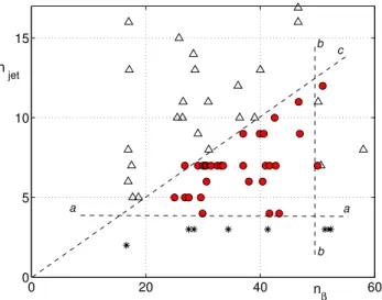
0 20 40 60 0
5 10
15 b
c
b a a
nβ n jet
Fig. 2. Parameter space of different flow regimes inβ-plane tur-bulence. The vertical axis shows the number of jets,njet, which
is equal to the wave number with the maximum energy. The filled (red) dots mark simulations in which the zonostrophic regime with
CZ≃0.5 had been established; the unfilled triangles and stars show
simulations lacking the universal regime. The large right triangle formed by the dashed lines delineates the parameter range con-ducive to the establishment of the zonostrophic regime.
important, therefore, to specify a relatively large dissipation capable of fully suppressing the enstrophy range (Maltrud and Vallis, 1991; Sukoriansky et al., 1999, 2002).
2.9 The small-scale forcing in 2-D simulations
In real systems, the energy sources are always related to 3-D processes. Since these processes are excluded in purely 2-D simulations, the forcing is introduced artificially, via random excitation of a number of small scale modes. Given computer limitations on the number of modes that can be resolved, such forcing may be acting on scales strongly affected by a β-effect which would result in loss of universality of the flow field. The issue (iii) above pertains to precisely such situa-tion and is concerned about the relative locasitua-tion of the forc-ing and transitional wave numbers,kξ andkβ, respectively.
We have investigated this issue in a new series of simulations and found out that for the establishing of the zonostrophic regime it is necessary thatkξ be sufficiently larger thankβ
as described in the next section, otherwise the emerging flow regimes are prone to a non-universal behavior. This condi-tion can be understood as a requirement that the forcing acts on relatively small scales where aβ-effect is weak.
2.10 A parametric study of the zonostrophic regime A new series of simulations was dedicated to studies of the nature of various steady-state regimes in a wide range of pa-rameters. A comprehensive description of these simulations will be given elsewhere; here, we provide a brief summary of
the pertinent results. Recall that the steep zonal spectrum re-sults in a very slow evolution of the flow field; a fact already noticed in unsteady simulations. Ifτis the characteristic time scale of the (linear) large-scale drag, then the establishment of a steady state has a duration of about 10τ, while to as-semble sufficient statistics for spectral analysis, one needs to extend the integration to about 100τ(Galperin and Sukorian-sky, 2005). All simulations performed in our new study had a duration between 35τ and 100τ. The friction time scale,τ, can be related to a large-scale friction wave number,nf r, if
we notice that a typical zonal spectrum in steady-state sim-ulations features a steep inertial range and a relatively flat plateau at the smallest wave numbers affected by the large-scale friction. The wave number,nf r, can be identified with
the transition from the steep spectral slope to the plateau and quantified in terms ofτ (Galperin et al., 2001; Sukoriansky et al., 2002). In some cases,nf rcan be associated either with
the wave-number at whichE(n)attains its maximum value or withnjet, the number of the alternating jets.
Our simulations have revealed that the parametric range admitting a steady-state zonostrophic regime withCZ≃0.5
is restricted by the following conditions:
(I) the forcingξ acts on relatively small scales only weakly affected by theβ-related anisotropy, such thatnξ/nβ&2;
(II) the extent of the inertial range should be large enough, nβ/nf r&4;
(III) the large-scale drag should be relatively small yet large enough to prevent the accumulation of energy in the largest available modes, such thatnf r>3 (in units of a sphere with
R=1);
(IV) the small-scale dissipation should be large enough to virtually suppress the enstrophy subrange, i.e., the ratio of characteristic length scales of the dissipation and the forcing, nξ/nd, should be slightly smaller than 1. The characteristic
dissipation length scale, 1/nd, can be determined by
equat-ing its characteristic time scale to that of a wave-number somewhat larger thannξ. Then, the dissipation parameters
can be adjusted in such a way as to attain the desirable target value of the rationξ/nd. In our simulations, this ratio was
kept close to 0.7.
Summarizing the criteria formulated in (I)–(III), one ar-rives at a chain inequality delineating the parametric range of the zonostrophic regime:
nξ &2nβ &8nf r &30. (16)
The criterion (IV) is important for purely 2-D simulations but has less significance in real flows where the energy sources are almost always associated with scales affected by three-dimensionality and vortex stretching.
regime withCZ≃0.5. On the other hand, the unfilled
trian-gles and stars pertain to flows in which at least one of the criteria (I)–(IV) was violated. All such flows were found to lack universal behavior. Most of the simulations by Danilov and Gryanik (2004) and Danilov and Gurarie (2004) belong in the latter group. In addition, all of their simulations were almost certainly of insufficient duration to enable “universal” flows to develop to full maturity. We have replicated some of these simulations; those satisfying criteria (I)–(IV) produced smoother spectra, Eqs. (7), (8), with CZ≃0.5 when
aver-aged over longer times. Note that in all simulations with the zonostrophic regime, the flow field exhibited slow variability which yielded, upon long-time averaging, smooth zonal and residual spectra. This result points to the stochastic nature of the flow field. In the framework of a general theory, the issue of stochasticity has important implications for the universal-ity of the flow regime. Clearly, if the large-scale structures were quasi-deterministic, as asserted in Danilov and Gurarie (2004) and Danilov and Gryanik (2004), then the quest for the universal statistical behavior would be meaningless.
It is of interest to find out about the fate of the “moving energy front,” Eq. (12), and the Rhines scale, Eq. (10), in steady-state flows. Recall that in such flows, the zonal spec-trum is comprised of the steep inertial part given by Eq. (7) forn>nf r and an approximate plateau forn<nf r. Noting
that in flows with a well developed spectrum (7) most of the energy is contained inEZ(n), their total kinetic energy is
es-timated by integrating this spectrum from 0 to∞(Galperin et al., 2001),
Etot=(5CZ/4)(/R)2n−f r4. (17)
Explorations of the planetary energetics based upon Eq. (17) are given in Galperin et al. (2001) and Sukoriansky et al. (2002). Substituting U=(2Etot)1/2 in the definition of the
Rhines’s number,nR=(β/U )1/2, and replacingβ by/R,
we obtain
nR=
5 4CZ
−1/4
nf r ≃nf r. (18)
A comparison of this result with Eq. (10) shows that, while in unsteady flowsnRdesignates the moving energy front, in
steady-state flows the advance of this front is terminated by the large-scale friction at wave numbernf r at which point
the spectrum flattens out. The wave numbersnf r≃nRshow
the “final destination” of the moving energy front; they both demarcate the low wave-number terminus of the spectral range with the−5 slope. Note that since the spectrum (7) is very steep, most of the energy is concentrated in the lowest modes with the−5 spectrum, i.e., around the wave-number nf r. Therefore,nf r determines the signature of the
veloc-ity profile and, thus, the number of the zonal jets (Galperin et al., 2001). Using unforced inviscid simulations on a rotat-ing sphere, Menou et al. (2003) have estimated the number
Fig. 3.Schematic representation of energy transfers in a two-layer system (after Salmon, 1998, and Read, 2005).
of zonal bands/jets asNband∼1/(2Ro)1/2, where the Rossby
number,Ro, is given by Ro≡ U
R. (19)
EvaluatingU, as before, from Eq. (17) and substituting it in Eq. (19), we findNband≃Rnf r thus demonstrating the
con-sistency between our definitions of the number of zonal jets and that of Menou et al. (2003). However, since the spectra have not been computed in Menou et al. (2003), it is difficult to judge whether or not the zonostrophic regime was attained in those simulations.
3 Barotropic mode in stratified flows
The flows considered so far were idealized, two-dimensional and barotropic. Real-world flows are more typically three-dimensional and baroclinic. Would it not be an over-simplification to seek for characterization of the latter by the former? Consideration of the normal-mode representa-tion allows one to establish an appropriate framework for such a characterization. In accordance with the Taylor-Proudman theorem, strong rotation results in a tendency to-wards two-dimensionalization of planetary flows on large scales. On even larger scales, theβ-effect leads to horizontal anisotropization and zonation. As demonstrated by Salmon (1998) on an example of a two-layer system (see also Rhines, 1979; Read, 2001, 2005) and schematically represented on Fig. 3, large-scale thermal forcing, via baroclinic instabil-ity at the scales of the first baroclinic deformation radius LRo∝1/nRo, leads to energy transfer to a barotropic mode
which is independent of vertical coordinate and, thus, be-haves like 2-D turbulence. If the baroclinic-barotropic en-ergy conversion takes place on sufficiently small scales, and the radius of the planet is sufficiently large, i.e., the Burger number is small, Bu≡(LRo/R)2≪1, then the barotropic
2.0 m 4.5 m
55cm 20cm
rotating spray arm
laser light sheet
Fig. 4.Schematic cross-section of the experimental rig used for the Grenoble experiment to demonstrate anisotropic zonation.
n<nRo and, thus, acquire features of barotropic 2-D
turbu-lence with aβ-effect. The criteria (I)–(IV) identified in the previous section as necessary conditions for the development of a universal flow regime in steady-state simulations can now be applied to the barotropic mode. Let us assume that even if the flow has additional forcing mechanisms that dif-fer from the baroclinic instability, their scale does not exceed LRo, i.e.,nξ&nRo. Using this assumption, we can extend the
criterion (16) to the barotropic mode of baroclinic flows, nξ &nRo&2nβ &8nf r &30. (20)
The chain inequality (20) sharpens the criterionBu≪1 and rectifies the conditions that can bring to life the zonostrophic flow regime.
Let us now turn to validating the criterion (20) versus data collected in laboratory experimentation and from observa-tions of the large-scale planetary and terrestrial circulaobserva-tions. Flows with small Bu and a topographic β-effect have re-cently been created in the world’s largest rotating tank, the Coriolis turntable, in Grenoble, France. The Grenoble ex-periment will be described in detail in the next section. In the natural environment, flows with small values ofBuand nf r/nβ abound in the atmospheres of the outer planets and
in the terrestrial oceans. These flows are analyzed in Sects. 5 and 6, respectively.
4 The Grenoble experiment
While results from clean and carefully formulated idealized numerical experiments can provide valuable insights from the viewpoint of basic theory, various assumptions made in their formulation need to be tested and evaluated under more physically realizable conditions. Laboratory experi-ments provide the best well-controlled environment in which to investigate dynamical phenomena in a real fluid, provided appropriate dynamical similarity can be achieved. In the case of turbulent zonation on aβ-plane, although a basic analog of the β-plane can be produced in a rotating fluid by use
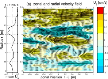
−0.5 0 0.5 3 3.5 4 4.5 5 5.5 6 6.5
Radius r [m]
mean Uθ
t = 11480 s Uθ [cm/s]
−1 −0.8 −0.6 −0.4 −0.2 0 0.2 0.4 0.6 0.8 1
−1 −0.8 −0.6 −0.4 −0.2 0 0.2 0.4 0.6 0.8 1 3
3.5 4 4.5 5 5.5 6 6.5
(a) zonal and radial velocity field
Zonal Position r ⋅θ [m]
Fig. 5. Instantaneous velocity field and zonal flow profile (in cm s−1) as a function of radius during the development of zonation in a convectively driven flow on a topographicβ-plane.
of sloping bottom topography, the requirements for dynami-cal similarity in the laboratory turn out to be very stringent, particularly with regard to achieving conditions under which viscous friction is sufficiently weak to allow for a significant turbulent inertial range to develop. Thus, although some hint of zonation effects has been evident in several small-scale ex-periments in the past (Mason, 1975; Bastin and Read, 1998; Sommeria et al., 1991), none of these were able to produce fully-developed zonal jets and anisotropic spectra exhibiting the properties discussed above, mainly because viscous dis-sipation was too strong and exerted a significant influence even at the energy injection scales (produced either by forced source-sink vortices or baroclinic instability).
Recently, Read et al. (2004) have conducted an experi-ment in a very large (13 m diameter) rotating tank with both strong rotation and a topographicβ-effect. The small-scale forcing was delivered via unstably-stratified convection, pro-duced by carefully spraying a continuous film of dense, salty water over the water surface. This generated a field of small convective plumes with a horizontal scale of around 15 cm, which were transformed into vortices via interaction with the background rotation. The basic experimental arrangement is illustrated in Fig. 4. A sloping bottom with depth increas-ing with radius (see Fig. 4) was produced with a stretched fabric sheet mounted on a conical tubular frame in the base of the tank. Both downward sloping and flat bottom config-urations were investigated (though a slight upward slope in the free upper surface was unavoidable due to the centrifu-gal distortion produced by the background rotation; but this never exceeded 0.6◦at mid-radius).
rotated at up to=π/20 rad s−1, corresponding to a Burger
numberBu∼5×10⁻⁴, and the forcing maintained for up to
4–6 h continuous operation.
When a flat bottom was used, the convective eddies were found to grow in size during the initial development of the flow until the annular channel was occupied by a small num-ber of weak domain-filling vortices, superimposed upon a broad, weakly retrograde zonal flow produced by residual wind-stress effects at the free upper surface. When a 5◦ sloping bottom was used, however, the vortex field which developed from the initial convection grew to a maximum size of around 1 m, in association with a persistent pattern of alternating prograde and retrograde zonal jets, also with a radial spacing of around 1 m. An example of this zonally-organized flow is shown in Fig. 5, in which the azimuthal flow is contoured and velocity vectors superposed at around the mid-depth of the tank. The coherent pattern of parallel, zonally-oriented jets is clear, with an amplitude of around 0.5 cm s−1.
Despite the baroclinic nature of the convective forcing, the rotationally-modified response, at least on large scales, was strongly barotropic. Figure 6 shows horizontal maps of the kinetic energy of the vertically averaged flow and that of the vertically-varying fluctuations for an example of a fully de-veloped flow (in fact with a flat bottom, though similar results were also obtained with a sloping bottom), measured by PIV at 5 levels in the vertical spanning the depth of the tank. The horizontal (vector) velocity field was first averaged in the ver-tical at each horizontal grid point and the mean and standard deviation of each velocity component was then used in turn to compute maps of vertical mean kinetic energy and that of the vertically-varying fluctuations. The fluctuation field is much less energetic than the mean field and is dominated by small scale features (with a typical diameter of 10–15 cm), repre-senting the scales of the individual convective plumes. In contrast, the mean field is at least 5–10 times more energetic than the fluctuations and evidently dominated by large scales, representing the rotationally-modified field of barotropic jets and vortices.
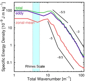
The clear change in the zonal structure of the horizontal flow by imposing the sloping bottom topography was also re-flected in the kinetic energy spectra. Figure 7 shows the time-mean spectrum obtained with a sloping bottom, in which the total kinetic energy density (integrated over all directions) decreases with increasing wavenumberk, but saturates to a near constant value fork less than a limiting value (corre-sponding roughly to a frictional wavenumberkf r). The eddy
contribution to the kinetic energy density shows an initial spectral slope (betweenk=15 and 30 m−1, cf. an energy in-jection scale of aroundkξ=40 m−1) corresponding roughly
to the classical−5/3KBK spectrum. In contrast, the zonal
mean spectrum (along thekθ=0 axis, whereθ is azimuth)
initially shows a much steeper fall-off beyond akf rof around
10 m−1, with a gradient of around−3 to−5, approaching the
−5 suggested by the predictions of the theory above.
More-Fig. 6. Instantaneous (horizontal) kinetic energy field and fluctua-tions at mid-depth as a function of radius and azimuth during the development of a convectively driven flow with a flat bottom in the Grenoble experiment (Read et al., 2004).
over, the magnitude of the zonal mean kinetic energy spec-trum is also roughly consistent with CZ≃0.5 as suggested
above, as indicated by the solid line with slope−5 in Fig. 7. These trends were not evident in the flat bottom case (cf. Read et al., 2004), for which the spectrum was generally shallower than the KBK−5/
3slope and the zonal spectrum
was dominated by wind-stress effects, greatly exceeding the strength suggested from the theory outlined above.
Although the spectra and other features of the sloping bottom experiment exhibit various characteristics of the anisotropic flow regime introduced above, they also exhibit various other features which depart from this ideal behav-ior. This is not unduly surprising, given the difficulties in satisfying the criteria represented by Eq. (20) under labo-ratory conditions, even on the largest available experimen-tal facility. By use of the convective forcing mechanism, kξ∼kRo∼40 m−1. The frictional wavenumber seems to
0.1 1 10 100
1 10 100
Specific Energy Density [10
−
9
J m kg
−
1
]
Total Wavenumber [m
−1]
−8/3
Rhines Scale
−5/3
−3
−5 total
eddy
zonal-mean
Rhines Scale
Fig. 7.Time-averaged (horizontal) kinetic energy spectra for fully-developed flows with a sloping bottom in the Grenoble experiment (Read et al., 2004).
effects are dominated by scale-invariant laminar Ekman bot-tom friction. The conditions concerning kβ, however, are
more problematic. Based on an estimate ofǫ∼5×10⁻¹⁰m2 s−3(∼one quarter of the ratio of the measured total kinetic
energy and the Ekman spin-down timescaleτE),kβ is
esti-mated at around 15 m−1. Given thatk
f r∼10 m−1, this leaves
little room to obtain a fully developed, anisotropic, inverse energy inertial range. Moreover, the maximum duration of the experiments of 4–6 h was probably insufficient to allow the turbulent flow field to evolve to full maturity. Neverthe-less, it seems clear that this experiment has come the closest so far in the laboratory to achieving the conditions required for the zonostrophic flow regime dominated by a topographic β-effect. It will be difficult to improve significantly upon this experiment in the future unless the rotation rate can be sub-stantially increased, which is a significant engineering chal-lenge.
5 Anisotropic turbulence and large-scale circulation on giant planets
Large-scale circulations in the cloud layers of the outer planets are good candidates for the development of the zonostrophic flow regime for the following reasons:
(1) large-scale planetary flows are two-dimensionalized due to the actions of strong rotation and weak density stratifica-tion;
(2) the outer planets are gaseous and do not have solid boundaries, their large-scale friction is therefore relatively low;
(3) convective cells, solar and/or internal heating may pro-vide the necessary small-scale forcing that would give rise to an anisotropic inverse energy cascade towards planetary scales;
(4) the Burger number is small for all outer planets. This issue requires some clarification. According to Menou et al. (2003), for example, a Burger number, based upon an
externaldeformation radius,LE, is smaller than 5.6×10⁻²
for all giant planets. Note, however, that LE (given by
LE=(gD)1/2/f, where g is the gravity acceleration and
D is the pressure scale height of an atmospheric layer) represents the length scale of geostrophic adjustment in the shallow water approximation (Gill, 1982). The analysis in Sect. 3 employsBu calculated for the firstinternal (baro-clinic) deformation radius, LD, characterizing the scale of
baroclinic instability and defined asLD=N H /f, whereN
is the Brunt-V¨ais¨al¨a frequency andHis the depth of a stably stratified layer. Using an estimateN∼[(g/ρ0)(|1ρ|/H )]1/2,
whereρ0 is the reference density and|1ρ| is a measure of
the density deviation from the adiabatic lapse rate across the stable layer, find thatLD/LE∼[(H /D)(|1ρ|/ρ0)]1/2. Since
for most situations,H /D<1 and|1ρ|/ρ0≪1, one concludes
that LD/LE<1. In the absence of any knowledge of the
deep vertical stratification on the giant planets, one cannot determine accurate values of that ratio; however, a rough estimate,LD/LE∼1/10, is sufficient and plausible enough
for the present purposes. For comparison, for Jupiter, for example, the Galileo Probe found evidence for weakly stable stratification (≤0.1 K km−1) averaged over the 1–20 bar
range in pressure (Magalhaes et al., 2002). This would suggest a first baroclinic deformation radius of no more than a few thousand km, implying a Burger number of∼3×10⁻³ or less (an estimate of the same order of magnitude has been given by Li et al. (2006) based upon a number of studies over the last 25 years). Similar conditions are likely to prevail on the other outer planets. The small values ofBu leave open the possibility for flow barotropization and development of the anisotropic inverse cascade in the barotropic mode; (5) the inertial range is large sincenβ/nf r&10;
(6) smallnf rallows for considerable energy accumulation in
the barotropic mode. The barotropic mode is thus expected to dominate the cloud movement and determine the shape of the cloud tracks.
100 101 10−10 10−8 10−6 10−4 n 10 0 101 10−5 10−4 10−3 10−2 n −400 0 400 90S
45S EQ 45N 90N
0 200 400 90S
45S EQ 45N 90N
−100 0 100 200 90S 45S EQ 45N 90N Latitude
100 101 10−10 10−8 10−6 10−4 n E(n)
Saturn Neptune
U(m/s) Jupiter
U(m/s) U(m/s)
Fig. 8.Top row: observed zonal profiles deduced from the motion of the cloud layers (Garc´ya-Melendo and S´anchez-Lavega, 2001; S´anchez-Lavega et al., 2000; Sromovsky et al., 2001); bottom row: observed zonal spectra (solid lines and asterisks) and theoretical zonal spectra, Eq. (7) (dashed lines) on the giant planets [all spectra are normalized with their respective values of(/R)2].
of the spectra and the planetary energetics can be found in Galperin et al. (2001); Sukoriansky et al. (2002); Galperin and Sukoriansky (2005).
5.1 Equatorial jets
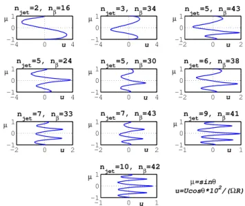
Numerous simulations with the 2-D vorticity equation on the surface of a rotating sphere have consistently produced westward equatorial jets (Cho and Polvani, 1996; Huang et al., 2001) although some of the simulations by Huang and Robinson (1998) did yield eastward jets. The westward jets are consistent with the circulation patterns on Uranus and Neptune, but they are opposite to the equatorial jets observed on Jupiter and Saturn. The seeming inability of the 2-D mod-els to produce eastward equatorial jets could indeed be a se-rious limitation of these models (Vasavada and Showman, 2005; Li et al., 2006). One of the issues investigated in our series of new long-term simulations described in the section 2.6 and shown in Fig. 2 was the direction of the equatorial jets which developed; the results are summarized in Fig. 9. The simulations revealed that the flow pattern was slowly meandering as a whole in the north-south direction such that the equatorial jets could be either eastward or westward; there were even situations when the equatorial velocity was zero. Slow fluctuations of the flow field are manifestation of the stochastic nature of turbulence with aβ-effect. To fully explore the question of stochasticity of the large-scale cir-culation on giant planets, long observational records, of the order of the time scale of the large-scale friction, would be required. However, such data is a matter of the remote future.
−4 0 4
−1 0 1
−2 0 2
−1 0 1
−2 0 2
−1 0 1
−2 0 2
−1 0 1
−1 0 1
−1 0 1
−1 0 1
−1 0 1
u
−4 0 4
−1 0 1
−4 0 4
−1 0 1
−4 0 4
−1 0 1
−2 0 2
−1 0 1
µ=sinθ u=Ucosθ*102/(ΩR)
n
jet=3, nβ=34 njet=5, nβ=43
njet=5, nβ=24 njet=5, nβ=30 njet=6, nβ=38
njet=7, nβ=33 njet=7, nβ=43 n
jet=9, nβ=41
n
jet=10, nβ=42 µ µ µ µ µ µ µ µ µ µ n
jet=2, nβ=16
u u u
u u u
u u u
Fig. 9.Zonal velocity profiles for different combinations ofnjetand nβfrom various long-term simulations using 2-D vorticity equation
on the surface of a rotating sphere.
An interesting insight into this problem from the viewpoint of the large-scale turbulence dynamics could be gained in the near future from the spectral analysis of the high-resolution circulation data collected by the Cassini mission for Jupiter and Saturn. A mission similar to Cassini could provide the same kind of data for Uranus and Neptune (Beebe, 2005).
Summarizing, let us emphasize that the existing opinion that the equatorial jets produced in barotropic simulations are always directed westward is fallacious although a certain preference to the formation of westward jets has been no-ticeable. Note also that the simulated equatorial jets are not necessarily symmetric with respect to the equator; this fact has been addressed in some discussions of the circulation on Uranus (Karkoschka, 1998; Hammel et al., 2001, 2005; Sro-movsky and Fry, 2005).
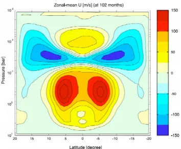
Fig. 10.Meridional cross-section through a baroclinic equatorial jet in an idealized 3-D numerical simulation of Jupiter’s upper tropo-sphere and stratotropo-sphere by Yamazaki et al. (2005).
variations may be due in part to fluctuations in cloud height as well as actual variations in the strength of the equatorial jet.
In an attempt to take this detailed structure into account, Yamazaki et al. (2005), for example, have recently pro-duced a baroclinic equatorial jet in numerical simulations involving angular momentum transport by both zonally-symmetric latitude-dependent heating (a Hadley circulation) and equatorially-trapped Kelvin waves. Figure 10 shows the result of such a combination of Hadley and Kelvin wave pro-cesses in producing a complex zonal velocity profile at cloud levels with a local minimum on the equator, much as ob-served. It does, however, imply a strongly baroclinic struc-ture below the clouds, for which there is as yet little observa-tional evidence either way.
6 The ocean-Jupiter connection
Eddy-permitting simulations of general oceanic circulation have consistently revealed systems of subsurface narrow zonal jets filling the entire ocean domain; see, e.g., Treguier et al. (2003) for the Atlantic, Nakano and Hasumi (2005) for the North Pacific, and Maximenko et al. (2005) for the global ocean. The signature of narrow zonal jets has also been detected in the maps of the surface geostrophic currents obtained from satellite altimetry (Maximenko et al., 2005). Comparing the visual appearance of the alternating zonal jets on the outer planets and in the ocean, Fig. 11, Galperin et al. (2004) have questioned whether or not their resemblance could be more than just coincidental. To answer this ques-tion, a spectral analysis of a 5-year long model-generated dataset of the North Pacific circulation (Nakano and Hasumi,
Fig. 11. (a)Composite view of the banded structure of the disk of Jupiter taken by NASA’s Cassini spacecraft on 7 December 2000 (image credit: NASA/JPL/University of Arizona);(b)zonal jets at 1000 m depth in the North Pacific Ocean averaged over the last five years of a 58-year long computer simulation (Nakano and Hasumi, 2005). The initial flow field was reconstructed from the Levitus cli-matology; the flow evolution was driven by the ECMWF climato-logical forcing. Shaded and white areas are westward and eastward currents, respectively; the contour interval is 2 cm s−1.
2005) was performed. In order to facilitate this calculation, a 60◦longitude sector of the Pacific was extracted from the original simulation. This sector was repeated 6-fold in the northern hemisphere, mirror-reflected relative to the equa-tor and repeated 6 more times in the southern hemisphere so as to assemble a continuous quasi-global dataset on the sphere. A spectral analysis of this dataset was performed us-ing the spherical harmonics decomposition; it yielded both zonal and residual spectra (Galperin et al., 2004). The cal-culated spectrum was averaged over the last 5 years of a 58-year long integration which was initialized using the Levi-tus climatology. As the simulated jets exhibit an equivalent barotropic structure, the analysis is based on the vertical av-erage from the surface to 500 m depth (as noted in Picaut and Sombardier (1993) and Wunsch (1997), the density field in the top 600 m of the water column is most important in com-putation of the normal modes). The results of the spectral analysis are shown in Fig. 12. The averaged zonal and non-zonal oceanic spectra are presented in Fig. 12a. A−5 slope is immediately evident for the zonal flows. Similarly to the case of giant planets (Figs. 12b and c), this slope extends up-ward to the dominant scale of the zonal jets yet for smallern the spectrum becomes flat. The universality ofEZ(n)is
sup-ported not only by the−5 slope, but also by the constancy of CZ≃0.5 for all cases. The energy spectrum for the nonzonal
components,ER(n), exhibits a slope close to−5/3over the
rangen=60−120. The departure ofER(n) from the−5/3
Fig. 12. Averaged and instantaneous zonal (thick solid lines) and non-zonal (thin solid lines) energy spectra on rotating planets with smallBu(top row) and in barotropic 2-D simulations on a rotating sphere Sukoriansky et al. (2002) (bottom row); the high wave num-ber spikes on the latter correspond to the small-scale forcing. All spectra are non-dimensionalized such thatEZ(1)=CZ. Idealized
−5 (thick dashed lines) and−5/3(thin dashed lines) slopes are
su-perimposed, based upon Eqs. (7) and (8), withCZ≃0.5,CK≃5 and
ǫ≃10−10m2s−3.
spectrum being about an order of magnitude larger. This re-sult is consistent with our Fig. 12a. We would also emphasize that both zonal and residual spectra of the horizontal currents have been obtained here from fully 3-D, realistic simulations of the circulation in the north Pacific rather than from ide-alized barotropic 2-D simulations used so far in theoretical studies. Note in addition that the barotropization on the lat-itudinal scale of the zonal jets’ width expected in flows with small Bu has been detected in simulations (Panetta, 1993; Williams, 2003; Nakano and Hasumi, 2005) as well as in ocean observations (Hall et al., 2004).
The spectraEZ(n)andER(n), obtained from a model of
2-D flow on a rotating sphere (Sukoriansky et al., 2002), are shown in Fig. 12e for comparison; they are averaged over about 300 years. As could be expected, longer averaging pro-duces smoother spectra. Since, as can be shown by simple energy balance arguments (Galperin et al., 2001), the char-acteristic time of the large-scale variability on Jupiter and Saturn is larger than the time of observations, the observed zonal spectra on these planets, presented on Figs. 12b and c, are, in fact,instantaneousspectra. Finally, Fig. 12d (Sukori-ansky et al., 2002) shows a typical instantaneous zonal spec-trum from a 2-D simulation. Large-amplitude fluctuations are characteristic of all instantaneous spectra including those in the ocean (not shown here).
Table 1. Parameters of large-scale circulation in various natural flows∗.
Source nξ n∗∗β nf r Bu
Coriolis turntable 40 15 10 5×10⁻⁴ Oceans 400 110 60 6×10⁻⁵ Jupiter 1000 310 16 3×10⁻⁵ Saturn 500 270 8 4×10⁻⁵ Uranus 400 150 3 5×10⁻⁵ Neptune 500 140 3 6×10⁻⁵
∗All wave numbers are given in units of a sphere withR=1. ∗∗In calculation ofn
β it was assumed thatǫ≃10−8m2s−3for all
giant planets
7 Conclusions
We have demonstrated that there exists a parametric range in which 2-D turbulence with aβ-effect develops a universal flow regime coined here a zonostrophic regime. This para-metric range is outlined by the chain inequality (16) and is distinguished by the anisotropic composite energy spectrum, Eqs. (7), (8), with the coefficientsCZ≃0.5 andCK≃5 which
thus appear to be universal constants. This regime is main-tained by the anisotropic inverse energy cascade that leads to the emergence of a flow pattern of alternating zonal jets. The lateral extent and preferred scale of these jets are de-termined by the large-scale energy withdrawal mechanism which is not completely understood at the present time, see e.g. M¨uller et al. (2005).
A similar regime may develop in the barotropic mode of stably stratified, 3-D, real-world flows with small values of a Burger number which is based upon the first baroclinic de-formation radius. The criteria (16) or (20) should also be fulfilled for the 3-D flows. One needs to keep in mind, how-ever, that these conditions have been derived from purely 2-D flows which have their own specific peculiarities absent in real 3-D flows. Therefore, these criteria are expected to be somewhat less restrictive when applied to the real world flows. Table 1 provides a summary of the parameters typical of various natural flows; the data used in this table is from Read et al. (2004); Galperin et al. (2004) and Galperin et al. (2001). The values of the Burger number for the giant planets are calculated according to the data in Menou et al. (2003) using the estimateLR=LE/10, established in Sect. 5. The
Analyzing Table 1, we take note that the inertial range for the Grenoble experiment is fairly narrow. Despite this, the experiment serves to link together data from the outer plan-ets, the subsurface oceanic circulation and computer simula-tions and seems generally to confirm that all these flows are governed by strongly non-linear dynamics with anisotropic inverse energy cascade. In view of the limitations discussed in Sect. 4, it would be a real challenge to expand this, re-quiring e.g. to significantly change the radius of the turntable and/or its rate of rotation.
For the terrestrial oceans, the criterion (20) generally holds although the inertial range is quite narrow. Note that the large-scale friction for these flows is fairly large, leading to nf r∼60, so that it would be generally wrong to say that the
zonostrophic regime can only develop in low-friction sys-tems. In the terrestrial oceans, the prevalence of the zonal energy over its meridional counterpart is not as prominent as on the giant planets, and this explains a highly fluctuating pattern of oceanic circulation on mesoscales.
Table 1 shows that the criterion (20) is best satisfied for the outer planets. In fact, they appear to present nearly ideal gigantic natural laboratories where the zonostrophic regime can materialize and be studied in all its complexity. Due to the low large-scale friction, most of the kinetic energy of the planetary atmospheric circulation is concentrated in the lowest zonal modes forming a pattern of relatively few, very stable, alternating zonal jets, particularly on the ice giants Uranus and Neptune. Through cloud advection, these jets manifest themselves as bands of different colors observable from a great distance.
The last decade has been distinguished not only by signif-icant progress in understanding of the atmospheric circula-tion on giant planets of the Solar System but also by the dis-covery of many planets beyond it, the so-called extra-solar system planets, or, briefly, exoplanets. Thus, Jupiter, Sat-urn, Uranus and Neptune are no longer the only giant planets whose atmospheric circulation can be understood and quan-tified within a general theory. At the present time, there are 170 gaseous giant planets known to move around their Sun-like stars (Burrows, 2005; the web page where the ex-trasolar planets’ catalogue is maintained is at J. Schneider, http://www.obspm.fr/encycl/encycl.html).
The present state-of-the-art in this area of planetary sci-ence has been vividly presented by Guillot (2005), “We lie on the verge of a true revolution: With ground-based and future space-based transit search programs, we should soon be able to detect and characterize many tens, probably hun-dreds, of planets orbiting their stars, with hope of inferring their composition and hence the mechanisms responsible for the formation of planets.” This information may also enable us to characterize the large-scale planetary circulations, at least under some circumstances. In particular, if the circu-lation regimes of at least some of these planets are similar to the ones found on the giant planets of the Solar System, then, as follows from Eq. (17), only a few parameters will
be needed for their quantification. Those parameters are the planetary radius, the rate of rotation, and the frictional wave numbernf r. The mass and the radius of some of the
plan-ets can presently be measured with a fair degree of accuracy (Guillot, 2005). As explained earlier,nf r is roughly equal to
the number of bands on the planetary disc. This data, as well as the planetary rotation rates may become available from future space-based observations.
Finally, we note that a rigorous confirmation of the pres-ence of the inverse energy cascade in real flows requires com-putation of the data-based spectral energy transfer with rela-tively high resolution of the velocity field. Such an analysis has not been performed yet for either of the systems con-sidered here. However, for the oceanic flows, the first steps in this direction have been undertaken by Scott and Wang (2005). In addition to the zonal spectrum (7) it is important to have a good estimate of the residual spectrum (8) which is an important characteristic of the large-scale circulation in systems with a strongβ-effect. This spectrum can be com-puted for the Grenoble experiment and for the ocean. The current resolution and the surface coverage are insufficient to determineER(n)for the flows on the outer planets. One
may hope that this situation will dramatically improve when the data from the Cassini encounters of Jupiter and Saturn will become available, opening up numerous venues for in-terdisciplinary, laboratory-terrestrial-planetary studies.
Acknowledgements. The authors greatly appreciate helpful com-ments by R. Salmon. This research has been partially supported by the US Army Research Office, the Israel Science Foundation and the UK Particle Physics and Astronomy, and Natural Environment Research Councils.
Edited by: W.-G. Fr¨uh Reviewed by: two referees
References
Balk, A.: A new invariant for Rossby wave systems, Phys. Lett. A, 155, 20–24, 1991.
Balk, A.: Angular distribution of Rossby wave energy, Phys. Lett. A, 345, 154–160, 2005.
Basdevant, C., Legras, B., Sadourny, R., and Beland, M.: A study of barotropic model flows: intermittency, waves and predictability, J. Atmos. Sci., 38, 2305–2326, 1981.
Bastin, M. and Read, P.: Experiments on the structure of baroclinic waves and zonal jets in an internally heated rotating cylinder of fluid, Phys. Fluids, 10, 374–389, 1998.
Beebe, R.: Comparative study of the dynamics of the outer planets, Space Sci. Rev., 116, 137–154, 2005.
Boer, G.: Homogeneous and isotropic turbulence on the sphere, J. Atmos. Sci., 40, 154–163, 1983.
Boer, G. and Shepherd, T.: Large-scale two-dimensional turbulence in the atmosphere, J. Atmos. Sci., 40, 164–184, 1983.
Burrows, A.: A theoretical look at the direct detection of giant plan-ets outside the Solar System, Nature, 443, 261–268, 2005. Chekhlov, A., Orszag, S., Sukoriansky, S., Galperin, B., and
Staroselsky, I.: The effect of small-scale forcing on large-scale structures in two-dimensional flows, Physica D, 98, 321–334, 1996.
Cho, J.-K. and Polvani, L.: The emergence of jets and vortices in freely evolving, shallow-water turbulence on a sphere, Phys. Flu-ids, 8, 1531–1552, 1996.
Danilov, S. and Gryanik, V.: Barotropic beta-plane turbulence in a regime with strong zonal jets revisited, J. Atmos. Sci., 61, 2283– 2295, 2004.
Danilov, S. and Gurarie, D.: Scaling, spectra and zonal jets in beta-plane turbulence, Phys. Fluids, 16, 2592–2603, 2004.
Flasar, F., Kunde, V., Achterberg, R., Conrath, B., Simon-Miller, A., Nixon, C., Gierasch, P., Romani, P., B´ezard, B., Irwin, P., Bjoraker, G., Brasunas, J., Jennings, D., Pearl, J., Smith, M., Orton, G., Spilker, L., Carlson, R., Calcutt, S., Read, P., Taylor, F., Parrish, P., Barucci, A., Courtin, R., Coustenis, A., Gautier, D., Lellouch, E., Marten, A., Prange, R., Biraud, Y., Fouchet, T., Ferrari, C., Owen, T., Abbas, M., Samuelson, R., Raulin, F., Adel, P., Ce´sarsky, C. J., Grossman, K., and Coradini, A.: An intense stratospheric jet on Jupiter, Nature, 427, 132–135, 2004. Galperin, B. and Sukoriansky, S.: Energy spectra and zonal flows on theβ-plane, on a rotating sphere, and on giant planets, in: Marine Turbulence: Theories, Observations, and Models, edited by: Baumert, H., Simpson, J., and S¨undermann, J., pp. 472–493, Cambridge University Press, 2005.
Galperin, B., Sukoriansky, S., and Huang, H.-P.: Universal n−5
spectrum of zonal flows on giant planets, Phys. Fluids, 13, 1545– 1548, 2001.
Galperin, B., Nakano, H., Huang, H.-P., and Sukoriansky, S.: The ubiquitous zonal jets in the atmospheres of giant plan-ets and Earth’s oceans, Geophys. Res. Lett., 31, L13303, doi:10.1029/2004GL019691, 2004.
Garc´ya-Melendo, E. and S´anchez-Lavega, A.: A study of the stabil-ity of Jovian zonal winds from HST Images: 1995–2000, Icarus, 152, 316–330, 2001.
Gill, A.: Atmosphere-Ocean Dynamics, Academic Press, 1982. Guillot, T.: The interiors of giant planets: Models and
out-standing questions, Annu. Rev. Planet. Sci., 33, 493–530, doi:10.1146/annurev.earth.32.101802.120325, Annual Reviews, 2005.
Hall, M., Joyce, T., Pickart, R., Smethie Jr., W., and Torres, D.: Zonal circulation across 52◦W in the North Atlantic, J. Geophys. Res., 109, doi:10.1029/2003JC002103, 2004.
Hammel, H., Rages, K., Lockwood, G., Karkoschka, E., and de Pa-ter, I.: New measurements of the winds of Uranus, Icarus, 153, 229–235, 2001.
Hammel, H., de Pater, I., Gibbard, S., Lockwood, G., and Rages, K.: Uranus in 2003: Zonal winds, banded structure, and discrete features, Icarus, 175, 534–545, 2005.
Hasselmann, K.: A criterion for nonlinear wave stability, J. Fluid Mech., 30, 737–739, 1967.
Heimpel, M., Aurnou, J., and Wicht, J.: Simulation of equatorial and high-latitude jets on Jupiter in a deep convection model, Na-ture, 438, 193–196, doi:10.1038/nature04208, 2005.
Holloway, G.: Contrary roles of planetary wave propagation in atmospheric predictability, in: Predictability of Fluid Motions,
edited by: Holloway, G. and West, B., pp. 593–599, American Institute of Physics, New York, 1984.
Holloway, G. and Hendershott, M.: Stochastic closure for nonlinear Rossby waves, J. Fluid Mech., 82, 747–765, 1977.
Huang, H.-P. and Robinson, W.: Two-dimensional turbulence and persistent zonal jets in a global barotropic model, J. Atmos. Sci., 55, 611–632, 1998.
Huang, H.-P., Galperin, B., and Sukoriansky, S.: Anisotropic spec-tra in two-dimensional turbulence on the surface of a rotating sphere, Phys. Fluids, 13, 225–240, 2001.
Karkoschka, E.: Clouds of high contrast on Uranus, Science, 280, 570–572, 1998.
Kraichnan, R.: Eddy viscosity in two and three dimensions, J. At-mos. Sci., 33, 1521–1536, 1976.
Legras, B.: Turbulent phase shift of Rossby waves, Geophys. As-trophys. Fluid Dyn., 15, 253–281, 1980.
Lesieur, M.: Turbulence in Fluids, Kluwer, third edn., 1997. Li, L., Ingersoll, A., and Huang, X.: Interaction of moist convection
with zonal jets on Jupiter and Saturn, Icarus, 180, 113–123, 2006. Magalhaes, J., Seiff, A., and Young, R.: The stratification of Jupiter’s troposphere at the Galileo Probe entry site, Icarus, 158, 410–433, 2002.
Maltrud, M. and Vallis, G.: Energy spectra and coherent structures in forced two-dimensional and beta-plane turbulence, J. Fluid Mech., 228, 321–342, 1991.
Manfroi, A. and Young, W.: Slow evolution of zonal jets on the beta plane, J. Atmos. Sci., 56, 784–800, 1999.
Mason, P.: Baroclinic waves in a container with sloping end walls, Phil. Trans. Royal Soc. London, Ser. A, 278, 397–445, 1975. Maximenko, N., Bang, B., and Sasaki, H.: Observational evidence
of alternating zonal jets in the world ocean, Geophys. Res. Lett., 32, L12607, doi:10.1029/2005GL022728, 2005.
Menou, K., Cho, J. Y.-K., Seager, S., and Hansen, B. M. S.: “Weather” variability of close-in extrasolar giant planets, Astro-phys. J., 587, L113–L116, 2003.
M¨uller, P., McWilliams, J., and Molemaker, M.: Routes to dis-sipation in the ocean: the two-dimensional/three-dimensional turbulence conundrum, in: Marine Turbulence: Theories, Ob-servations, and Models, edited by: Baumert, H., Simpson, J., and S¨undermann, J., pp. 397–405, Cambridge University Press, 2005.
Nakano, H. and Hasumi, H.: A series of zonal jets embedded in the broad zonal flows in the Pacific obtained in eddy-permitting ocean general circulation models, J. Phys. Oceanogr., 35, 474– 488, 2005.
Panetta, R.: Zonal jets in wide baroclinically unstable regions: per-sistence and scale selection, J. Atmos. Sci., 50, 2073–2106, 1993. Pedlosky, J.: Geophysical Fluid Dynamics, Springer-Verlag, second
edn., 1987.
Picaut, J. and Sombardier, L.: Influence of density stratification and bottom depth on vertical mode structure functions in the tropical Pacific, J. Geophys. Res., 98, 14 727–14 737, 1993.
Read, P.: Transition to geostrophic turbulence in the laboratory, and as a paradigm in atmospheres and oceans, Surv. Geophys., 22, 265–317, 2001.
Uni-versity Press, 2005.
Read, P., Yamazaki, Y., Lewis, S., Williams, P., Miki-Yamazaki, K., Sommeria, J., Didelle, H., and Fincham, A.: Jupiter’s and Sat-urn’s convectively driven banded jets in the laboratory, Geophys. Res. Lett., 31, L22701, doi:10.1029/2004GL020106, 2004. Rhines, P.: Waves and turbulence on a beta-plane, J. Fluid Mech.,
69, 417–443, 1975.
Rhines, P.: Geostrophic Turbulence, Annu. Rev. Fluid Mech., 11, 401–411, 1979.
Salmon, R.: Lectures on Geophysical Fluid Dynamics, Oxford Uni-versity Press, 1998.
S´anchez-Lavega, A., Rojas, J., and Sada, P.: Saturn’s zonal winds at cloud level, Icarus, 147, 405–420, 2000.
S´anchez-Lavega, A., Perez-Hoyos, S., Rojas, J., Hueso, R., and French, R.: A strong decrease in Saturn’s equatorial jet at cloud level, Nature, 423, 623–625, 2003.
Scott, R. and Wang, F.: Direct evidence of an oceanic inverse kinetic energy cascade from satellite altimetry, J. Phys. Oceanogr., 35, 1650–1666, 2005.
Smith, L. and Waleffe, F.: Transfer of energy to two-dimensional large scales in forced, rotating three-dimensional turbulence, Phys. Fluids, 11, 1608–1622, 1999.
Smith, L. and Yakhot, V.: Bose condensation and small-scale struc-ture generation in a random force driven 2D turbulence, Phys. Rev. Lett., 71, 352–355, 1993.
Smith, L. and Yakhot, V.: Finite-size effects in forced two-dimensional turbulence, J. Fluid Mech., 274, 115–138, 1994. Sommeria, J., Meyers, S., and Swinney, H.: Experiments on
vor-tices and Rossby waves in eastward and westward jets, in: Non-linear Topics in Ocean Physics, edited by: Osborne, A., pp. 227– 269, North-Holland, Amsterdam, 1991.
Sromovsky, L. and Fry, P.: Dynamics of cloud features on Uranus, Icarus, 179, 459–484, 2005.
Sromovsky, L., Fry, P., Dowling, T., Baines, K., and Limaye, S.: Coordinated 1996 HST and IRTF imaging of Neptune and Tri-ton III. Neptune’s atmospheric circulation and cloud structure, Icarus, 149, 459–488, 2001.
Sukoriansky, S. and Galperin, B.: Subgrid- and supergrid-scale parameterization of turbulence in quasi-two-dimensional barotropic flows and phenomenon of negative viscosity, in: Ma-rine Turbulence: Theories, Observations, and Models, edited by: Baumert, H., Simpson, J., and S¨undermann, J., pp. 458–470, Cambridge University Press, 2005.
Sukoriansky, S., Galperin, B., and Chekhlov, A.: Large scale drag representation in simulations of two-dimensional turbu-lence, Phys. Fluids, 11, 3043–3053, 1999.
Sukoriansky, S., Galperin, B., and Dikovskaya, N.: Uni-versal Spectrum of Two-Dimensional Turbulence on a Ro-tating Sphere and Some Basic Features of Atmospheric Circulation on Giant Planets, Phys. Rev. Lett., 89(12), DOI:10.1103/PhysRevLett.89.124501, 2002.
Treguier, A., Hogg, N., Maltrud, M., Speer, K., and Thierry, V.: The origin of deep zonal flows in the Brazil basin, J. Phys. Oceanogr., 33, 580–599, 2003.
Vallis, G. and Maltrud, M.: Generation of mean flows and jets on a beta plane and over topography, J. Phys. Oceanogr., 23, 1346– 1362, 1993.
Vasavada, A. and Showman, A.: Jovian atmospheric dynamics: an update after Galileo and Cassini, Rep. Prog. Phys., 68, 1935-1996, doi:10.1088/0034–4885/68/8/R06, 2005.
Williams, G.: Jovian dynamics. Part III: Multiple, migrating, and equatorial jets, J. Atmos. Sci., 60, 1270–1296, 2003.
Wunsch, C.: The vertical partition of oceanic horizontal kinetic en-ergy, J. Phys. Oceanogr., 27, 1770–1794, 1997.
Yamazaki, Y., Read, P., and Skeet, D.: Hadley circulations and Kelvin wave-driven equatorial jets in the atmospheres of Jupiter and Saturn, Planet. Space Sci., 53, 508–525, 2005.