FACULDADE DE ECONOMIA
PROGRAMA DE PÓS-GRADUAÇÃO EM ECONOMIA - CAEN
YURI LACERDA COSTA
MODELING BAYESIAN UPDATING WITH MANY NON-UPDATERS: THE CASE OF OWN SUBJECTIVE HOMICIDE VICTIMIZATION RISK
FORTALEZA
MODELING BAYESIAN UPDATING WITH MANY NON-UPDATERS: THE CASE OF OWN SUBJECTIVE HOMICIDE VICTIMIZATION RISK
Dissertação de Mestrado apresentada ao Pro-grama de Pós-Graduação em Economia, da Faculdade de Economia da Universidade Fe-deral do Ceará, como requisito parcial para obtenção do Título de Mestre em Economia. Área de concentração: Métodos Quantitativos em Economia.
Prof. Dr. José Raimundo de Araújo Carvalho Júnior
Dados Internacionais de Catalogação na Publicação Universidade Federal do Ceará
Biblioteca da Faculdade de Economia, Administração, Atuária e Contabilidade
C876m Costa, Yuri Lacerda.
Modeling bayesian updating with many non-updaters: the case of own subjective homicide victimization risk / Yuri Lacerda Costa – 2015.
41 f.: il.
Dissertação (Mestrado) – Universidade Federal do Ceará, Faculdade de Economia, Administração, Atuária e Contabilidade, Programa de Pós-Graduação em Economia, Fortaleza, 2015.
Área de Concentração: Métodos Quantitativos em Economia. Orientação: Prof. Dr. José Raimundo de Araújo Carvalho Júnior.
1.Probabilidades 2. Teoria bayesiana de decisão estatística I.Título.
MODELING BAYESIAN UPDATING WITH MANY NON-UPDATERS: THE CASE OF OWN SUBJECTIVE HOMICIDE VICTIMIZATION RISK
Dissertação de Mestrado apresentada ao Pro-grama de Pós-Graduação em Economia, da Faculdade de Economia da Universidade Fe-deral do Ceará, como requisito parcial para obtenção do Título de Mestre em Economia. Área de concentração: Métodos Quantitativos em Economia.
Aprovada em 27 de Março de 2015.
BANCA EXAMINADORA
Prof. Dr. José Raimundo de Araújo Carvalho Júnior (Orientador)
Universidade Federal do Ceará
Prof. Dr. Sérgio Aquino de Souza Universidade Federal do Ceará
À minha psicóloga, Cecília Sena, pelo acompanhamento e zelo fundamentais neste período decisivo (e extremamente duro) da minha vida.
Ao Prof. José Raimundo, pela dedicação na orientação deste trabalho, bem como pelos inúmeros conselhos e esforços, sem paralelo, no desenvolvimento da minha carreira de pesquisador.
Aos meus pais, Luiz Cláudio e Adáuria, assim como ao meu irmão, Sued, pela compreensão e apoio durante esses dois anos turbulentos.
Aos meus colegas do LECO, em especial Diego de Maria André, pelas inúmeras vezes em que me socorreu com seu conhecimento sobre os softwares que tive que aprender usando neste trabalho.
Aos amigos Cristiano, Diego, Francisco, Gustavo e Júnior por tornar esses anos mais leves, especialmente nas horas do cafezinho.
Aos professores Henrique Félix, Jair do Amaral e Leandro Rocco pelo tempo que gentilmente me presentearam para conversas e conselhos de carreira.
Aos funcionários do CAEN, Adelino, Adriana, Carmem e Márcia pela prestatividade e simpatia que sempre demonstraram comigo.
Aos professores membros da banca examinadora, Leandro Rocco e Sérgio Aquino, pelo tempo empregado em contribuições valiosas a este trabalho.
Nosso principal objetivo neste estudo é investigar o papel da heterogeneidade na atualização, depois de um choque de informação, do risco subjetivo sobre vitimização de homicídio. Nesse sentido, os dados utilizados neste trabalho também atestam a superestimação do crime encontrada na literatura. A novidade é que os entrevistados receberam um choque de informação que consiste na taxa oficial de homicídios, mas a grande maioria deles mantém a mesma percepção inicial. Ao propor um modelo deUpdateBayesiano permitindo que nenhuma atualização fosse realizada, dois modelos foram desenvolvidos: um Tobit modificado e um modelo Hurdle de dois níveis. Assim como em estudos anteriores, nossos resultados mostraram que poderíamos prosseguir com uma abordagem deUpdateBayesiano. Ainda, quanto mais altas as respostas iniciais eram definidas, mais propensos os indiví-duos estavam em proceder uma mudança de percepção. Além disso, fundamentalmente, pudemos racionalizar a decisão de não revisar as respostas seguindo um argumento de qualidade/credibilidade da informação percebida. Descobrimos que os participantes mais velhos e as mulheres são mais relutantes não apenas em alterar as respostas iniciais, mas também na escolha do nível da nova resposta, em caso de mudança. Outra conclusão feita foi que o nível educacional dos entrevistados era insignificante em nosso exercício. De fato, o nível educacional do entrevistador teve um papel fundamental em ambas decisões de mudança e magnitude de revisão. Finalmente, nossos resultados também levantaram fortes evidências sobre aspectos de homofilia. A ocorrência de uma correspondência em gênero entre entrevistadores e entrevistados teve o maior impacto sobre a decisão de mudar e na magnitude da atualização neste estudo.
Our main purpose in this study is to investigate the role of heterogeneity into the update of subjective homicide victimization risk after an informational shock. In this sense, the data used here also attests the crime overestimation found in the literature. The novelty is that our respondents faced an informational shock consisting in the official homicide rate, but the vast majority of them keeps the same initial perception. In proposing a Bayesian Update model allowing that no update takes place, two models were developed: a modified Tobit and a two-tiered Hurdle model. In accordance with previous papers, our results showed that we could proceed with a Bayesian Update approach. Also, the higher initial responses are set, more likely individuals are in proceeding a change in perceptions. Furthermore, fundamentally, we could rationalize a non-updating decision following a perceived informational quality/credibility argument. We found that older participants and females are more reluctant not only to change initial responses, but also to choose the level of the new response, in case of an update. In addition, respondents’ level of education was insignificant in our exercise. In fact, interviewers’ level of education had a key role in both the changing and updating magnitude decisions. Finally, our results also raised strong evidence on homophily aspects. The occurance of a matching in gender between interviewers and interviewees had a major impact on the decision to change and in the magnitude of the update in this study.
2 LITERATURE REVIEW 4
2.1 Subjective Expectations and Bayesian Update . . . 4
2.2 Early Contributions . . . 6
2.3 Recent Developments . . . 9
3 DATA 13 4 ECONOMETRIC MODELS FOR BAYESIAN UPDATING 18 4.1 Classical Bayesian Update . . . 18
4.2 Multiple Linear Regression and Victimization Expectation Update . . . 19
4.3 Bayesian Updating with Skepticism . . . 20
4.3.1 Model 1: A Generalized Tobit for Bayesian Updating . . . 22
4.3.2 Model 2: A Simple Two-Tiered Hurdle Model . . . 24
5 RESULTS 25 5.1 Bayesian Update with Skepticism: Model 1 . . . 25
5.2 Bayesian Update with Skepticism: Model 2 . . . 26
1
INTRODUCTION
The last four decades of economic research are characterized by major advances in applied microeconomics. Issues previously restricted to other social sciences were being included into economists’ research agenda due to an increasing interest in interdisciplinary topics. This is the context in which the Economics of Crime emerged with the seminal paper of Becker (1968). In this paper, the author models the engagement in illegal activities as result of a rational decision following a cost/benefit analysis under a neoclassical perspec-tive. Based on this idea, discussions on deterrence and punishment strategies were raised designing public policies for crime control.
Apart from criminals, delinquency also involves a victim. In this sense, our study recognizes that the experience of crime itself is not the only input being processed. Also, the fear of being victimized plays a significant role in welfare and it is not unusual the occurrence of psychological disorders simply caused by a surge in crimes, developing seri-ous problems to individuals’ health and economic capability. However, it is important to note that becoming a victim is a rare event specifically focused on certain socioeconomic groups. Thus, given the importance of fear and the weak probabilistic justification for such a severe concern, understanding the factors underlying crime expectations and how information affect those risk perceptions is a gap we want to fill in.
In this sense, the standard economic analysis would suggest the use of probability distributions in order to deal with the uncertainty and risk involved in this situation. Nevertheless, there is an open debate on which type of distribution should be used: ob-jective or subob-jective. Works such as Gollier (2004) have been explaining risky decisions through the first option, while a growing line of research argues in favor of the last one. This defense is mainly motivated by the ideas of Behavioral Economics, a field initiated by Tversky & Kahneman (1974), among others, consisting in an intersection between Psychology and Economics.
Under this perspective, studies on consumers’ behavior were being added into an already consolidated Theory of Choice, overcoming unjustified and unnecessary assump-tions in many applicaassump-tions. This is the ground on which Manski (2004) presents a detailed defense in using subjective probabilities and measuring expectations in several situations such as schooling choices and perceptions of the returns to it. Hereupon, subjective per-ception of crime occurrence probabilities appears as an important tool for understanding victimization.
In summary, this dissertation, much in the spirit of the literature initiated by Viscusi (1979) in a labor market context, assumes that citizens are rational agents with imperfect information on the actual probability of becoming a crime victim. Nevertheless, they face information news about crime which is not necesserily credible on a daily basis in such a manner compatible with a learning process. Indeed, credibility is a key concept in our discussion and it is going to be explored in greater details from section (3) onwards.
the existence of non-updaters in a Bayesian Updating context. Furthermore, we search for observable characteristics in explaining a two-step decision: i) Changing or keeping initial perception; ii) Setting an update (if any). The empirical exercise is going to take place by means of heterogeneity in both sides of the informational interaction, i.e., sender and receiver, as well as in matching aspects between them.
As suggested by its name, the Bayesian approach — the one adopted in this disserta-tion — relies on the widely known Bayes’s theorem whose major contribudisserta-tion is to propose a link between current and past beliefs based on further evidence. Hence, situations in-volving initial perceptions followed by informational shocks are ideally suited for such analysis. However, since this approach fundamentally deals with subjective probabilistic beliefs, two relevant concerns arise: i) Are individuals able to think in terms of proba-bilities? ii) Are those responses reliable? Both questions pose resistance in working with subjective expectations, and some works, such as Hogarth (1975), provide a criticism on this reasoning. Nevertheless, there is strong evidence supporting the Bayesian approach in situations where the respondents faced relevant life aspects.
This is the case according to Viscusi & O’Connor (1984). The paper aims to inves-tigate if chemical industry workers learn about the risks they face on the job and how this understanding affects the reservation wages. The authors conducted a survey and col-lected information for 335 individuals of many different occupations to conclude that these workers update their probabilistic beliefs in a way which is compatible with a Bayesian procedure. This main result is also found in Viscusi (1985). The author argues that the Bayesian Update model is a useful optimization approach for analyzing economic behavior and, in some cases, even the existing bias can be predicted by applying the model itself.
An application of this technique in Health Economics is found in Smith & Johnson (1988) analyzing agents’ ability in processing information about the health risks of being exposed to a harmful substance. The main message brought by this paper is that the intoxication information which was neither recent nor relevant to the individual had in-significant effects on risk perceptions. On the other hand, this information seen as more updated and relevant appeared to be positively correlated to the posterior probability response. The authors also list four basic characteristics that a behavioral model — in some sense, what we want to propose — must consider:
i) The risky event’s importance for individuals interviewed;
ii) The role of prior beliefs regarding the risky event;
iii) The implications of new information on this process;
iv) The acquisition costs of this new information;
Twenty interviewers applied a questionnaire to 4,030 citizens of Fortaleza dealing with subjective expectations about being a victim of homicide on the following twelve months from the interview day onwards, among other issues. Apart from its size and information for both interviewees and interviewers, perhaps the most distinguished feature of this sample in the context of Bayesian Update is its vast majority of individuals who kept the same expectation, regardless the fact that their perceptions were far from official rates. We will refer to this behavior asSkepticism and to these respondents asSkeptical Agents. We found that around 95% of our participants decided not to move from initial per-ceptions, which is, by far, very different empirical evidence than what is found in the literature. Instead of questioning the rationality of individuals who decided not to update expectations in a learning context, we might be facing a skeptical agent in such a way that the informational content must be relevant enough to make a change in his perception. The results found in our study support this understanding. For example, in all models we proposed, the interviewers’ level of education, a central variable concerning the informa-tional quality, had positive coefficients into the changing decision. The same is implied by a matching variable in gender, whose positive coefficients tell us that informational noise reduction is favorable to an update.
The analysis presented in this dissertation is divided into six sections. Section (2) presents a brief discussion on subjective expectations and Bayesian Update. Then, it analyses the contributions of Viscusi & O’Connor (1984) seminal paper and its influence on Smith & Johnson (1988) with greater details. Finishing the section, a recent application of subjective expectations in Delavande (2008) is presented. Section (3) presents the data, emphasizing its advantages in comparison with previous papers and our major challenge: to deal with a very different sample in this context. Also, it brings an initial exploratory analysis, as well as a brief discussion on selection bias.
2
LITERATURE REVIEW
2.1
Subjective Expectations and Bayesian Update
The origins of Statistical Theory were mainly motivated by games of chance. At that time, not only determining the chances of a particular game result, but also inferring, given past evidence, some aspect of the game itself were questions underlying the work of many important mathematicians in the eighteenth century. In this context, the greatest contribution of Bayes & Price (1763), which was later improved by Laplace (1785), consists in a way to link the probability of a hypothesis, given past evidence, with the probability of that evidence, given the hypothesis. Formally, the famous Bayes’s theorem establishes that:
P(A|B) = P(B|A)P(A) P(B)
Despite an intense debate surrounding Frequentist and Bayesian approaches, it is out of our scope considerations of such nature in this study. However, since we are interested in updating subjective expectations, we recognize that the Bayesian structure emerges as a convenient interpretation for our purposes. Sivia (1996) presents a discussion that makes this connection more evident. The author argues that the probability we assign to the proposition “it will rain this afternoon”, for example, will depend on whether there are dark clouds or a clear blue sky in the morning; it will also be affected by whether or not we saw the weather forecast. In other words, individuals dealing with probabilities are assigning numbers to express beliefs on events occurrences, conditioning it to previous knowledge about the generating process.
Although the conditioning on information background is often omitted in calculations to reduce algebraic cluttering, we must never forget its existence. In this sense, we need a slight modification on notation to let explicit this fundamental Bayesian aspect: Prob-ability is not an absolute entity; it is an individual belief intrinsically conditioned to an informational set.
P(A|B, I) = P(B|A, I)P(A|I) P(B|I)
whereI is the conditioning informational set. Assuming that Ais theHypothesisand B
is theEvidence, and from the fact that P(Evidence|I) may be omitted1, we have:
P(Hypothesis|Evidence, I)∝P(Evidence|Hypothesis, I)P(Hypothesis|I)
This expression represents the core of a Bayesian Update model and its terms are defined and interpreted as follows:
P(Hypothesis|Evidence, I) : Posterior
The state of knowledge about the truth of a hypothesis given extra evidence about the event under consideration.
P(Evidence|Hypothesis, I) : Learning factor
A maximum Likelihood function.
1
P(Hypothesis|I) : Prior
The state of knowledge (or ignorance) about the truth of a hypothesis before any further evidence about the event under consideration.
Given the connection between initial perceptions and further evidence, the Bayesian appealingness for situations where agents possess incomplete information and are exposed to new informational bits is straightforward. Nevertheless, a previous step for its usage is of great resistance in Economics and Econometrics since, traditionally, information not objectively observed has little credibility2. Advocates of such understanding are based
in Samuelson (1938) defending that the only information needed and usable is that of behavior only3. Proceeding this way, it is possible to recover initial preferences and the
risk of making wrong assumptions about the introspection process is avoided. Also, it prevents any inconsistency raised by possible differences between what is said and done by the decision maker.
In this sense, the standard approach treats uncertain events occurrences as following an objective and known probability distribution. Based on this idea, Neumann & Morgen-stern (1947) shows the existence of a particular function form known as Expected Utility
Function. This result is intensively conjured up when modeling choice under uncertainty
and, whenever it is necessary to comment on the expectations formation process, the Rational Expectation assumption is taken, or, at least, bounded rationality. However, as pointed out by Pesaran (1987), Rational Expectations has not proven to be sufficiently convincing to analysis out of macroeconomic long-run even in its weaker version.
Manski (2004), accomplished an extensive survey referring to Manski (1993) in a returns return to the schooling context. The author argues that students face the same inferential problems that labor econometricians do. Therefore, since much debate is still in course among experts, it is implausible to assume that students share the same objective and correct distribution generating the returns.
The problem is that avoiding the assumption of unique objective probability existence, perfectly known and identically processed by all individuals, the standard analysis cannot take place. This is so because any specific choice result may arise by many different preferences and probabilities combinations. Hence, Manski (2004) presents a detailed defense in favor of using expectations self-reported in probabilistic terms, the so called
Subjective Probabilities4. This data type could be used to validate or relax hypothesis
used in the models.
In light of such perspective, several papers have successfully applied subjective prob-abilities in many situations where expectations are crucial in the analysis. For example, Manski have co-authored studies in income expectations (Dominitz & Manski (1997)), social security and retirement (Dominitz, Manski & Heinz (2002)), consumer confidence (Dominitz & Manski (2004)) among others. An application in survival expectations is presented in Hurd & McGarry (1995).
Once having raised the relevance of bringing subjective probabilities for discussion, criticisms about the reliability of this data type cannot be neglected. Thus, it is coherent that the first empirical studies had concentrated themselves primarily in situations involv-ing critical aspects for individuals under study, such as serious risks of health or death.
2
Much of this skepticism is explained by early data type usefulness criticism found in Machlup (1946) and Hart, Modigliani & Orcutt (1960).
3
An example of this acquaintance in Econometric Theory is found in McFadden (1973). 4
This is the context in which W. Kip Viscusi makes important contributions applying the Bayesian Update structure to model updating risk perceptions.
2.2
Early Contributions
Viscusi (1979), who was interested in the relation between risks for health and physical integrity at work and labor market outcomes, found that workers’ perceived risk has a positive correlation with the industry specific risk. Also, it shows that industries whose employees had higher risk perceptions presented higher wages as well, supporting the Compensating Differentials Theory. Therefore, understanding how risk perception evolves and how it is processed, shaping a new subjective probability distribution, emerges as a further step on the study of labor markets dynamics.
Interested in the relationship between perceived risks for health and physical integrity at work and labor market outcomes, Viscusi (1979) finds that workers’ perceived risk has a positive correlation with the industry specific risk. Also, it shows that industries whose employees had higher risk perceptions presented higher wages as well, supporting the Compensating Differentials Theory. Therefore, understanding how risk perception evolves and how it is processed, shaping a new subjective probability distribution, emerges as a further step on the study of labor markets dynamics.
Viscusi & O’Connor (1984) investigates whether employees revise their risk perceptions and, if so, how the reservation wage revision under a new informational set would be. Due to the lack of available data on workers’ risk perceptions evolution, the authors applied a questionnaire to 335 employees of three major American chemical industries. Workers were asked to mark their risk perception in a linear scale ranging from very safe to dangerous, with the US private sector accident and diseases rate presented as a reference point. Finally, answers were converted into probabilistic terms giving rise to the variable
RISK.
The study indicates that workers’ perceptions were consistent with the US private sector risk average, even though it is 50% above that of the chemical industry. Moreover, about one third of the sample believed having been exposed to risks above the national average. Although these results may seem contradictory, the authors argued that the national reference rate was based on accidents related to work safety, aspect in which the chemical industry had a favorable track record. Thus, these official statistics had under-estimated the long-term impacts on workers health due to chemical substances exposure. This evidence suggests some degree of a learning process.
In addition, Viscusi & O’Connor (1984) presents some models seeking to explain in-come based on standard variables such as race, education and experience, as well as those related to risk. This exercise allowed to identify risk premiums on wages, where these differentials ranged from $ 258.4 to $ 788.6, depending on the risk variable used and the subgroup analyzed. Finally, the results were consistently significant, in accordance with previous papers.
Since they were interested in the labor market dynamics, the authors created three other variables: QUITA, QUITB and TAKEA. The first two are related to decisions of leaving the job without transaction costs of searching for a new position. They differ from each other only regarding whether individuals consider themselves “inclined to make a
genuine effort to find a new job with a new employer next year” or “strongly inclined
(...)”, respectively. TAKEA refers to the decision of repeating the choice in accepting
of the sample would decide, without hesitation, to accept the same job, the probability
of TAKEAassuming value 1 is negatively related to all risk variables. Similarly, QUITA
had a positive relationship.
The first message of Viscusi & O’Connor (1984) is that the data is consistent with a model in which the choice of employment when facing risks is a learning process. Reser-vation wages grow as perceived risks increase, so that there is a risk premium keeping workers at their jobs until such compensation is not enough. From that point on, they decide to leave the job or, at least, not to accept the offer if this choice was put back.
The major contribution of this paper, however, is to investigate the informational shock effect on workers’ perceptions, which is exactly what we want to do in a victimization context. Following this purpose, the authors presented each worker a label containing information regarding a chemical substance that would replace the old products used in everyday work activities. Then, workers were asked to repeat their responses under this new information. There were four label types: CARB (Sodium Bicarbonate), LAC
(Lachrymator Chloroacetophenone),ASB (Asbestos) andTNT. As expected, the control groupCARB had a significant reduction in reported risk levels, virtually eliminating the chemical risk. As for LAC, ASB and TNT, employees reported risk levels almost three times higher and the vast majority believed having been exposed to above-average risks. Assuming that workers had a learning process which was consistent with a Bayesian approach, Viscusi & O’Connor (1984) models the initial risk perceptions, or thepriors, as following aBeta distribution. This particular choice was made considering the great free-dom allowed by this distribution, its ideal fit for independent Bernoulli experiments and the fact that a beta distribution is a conjugate prior5. Thus, the new labels were treated
as additional observations from bernoulli trials about suffering or not a work accident. The distribution parameters are p and γ, the initial probability of an unfavorable
out-come, i.e. RISK, and a term measuring this prior accuracy, respectively. After observing
m unfavorable (accidents) and n favorable (non accidents) results, the paper shows that the posterior, p∗, is given by:
p∗ = γp+m
γ+m+n (1)
The informational content of each label i depends on both the information accuracy, ξi, i.e. the equivalent m+n observations implied by this information, andsi = m
m+n, the
proportion of unfavorable observations. Thus, a label i increases the worker perceived risk when si is greater than pi and the correction magnitude is positively related to ξi.
Replacingξi andsi in (1), the posterior probability, p∗
i, of a work accident after receiving
a warning for the chemical i is given by:
p∗i = γp+ξisi γ+ξi =
ξisi γ+ξi +
γp
γ+ξi (2)
Therefore, from (2), an estimable linear form can be established as follows:
RISKli =αi+βiRISKi+ui
whereRISKli refers to the risk perception for substance iafter the informational shock
and ui is a random error term. This equation represents the Viscusi’s linear estimable
model of Bayesian Update.
5
The regression results show that the coefficientαi has a positive value andβi plays an
important role, so that workersposteriors have been influenced by both priors and label contents, creating a reviewing process consistent with the Bayesian approach. This is the starting point for our initial estimable model presented in subsection (4.2). For now, if we want to follow this idea for victimization updating expectations, our βi must also be
significant.
Motivated by Viscusi & O’Connor (1984), Smith & Johnson (1988) investigates how a sample of households in Maine, United States, responded to information regarding risks associated with radon concentration in their homes and water supplies. Whereas radon problems in the area had been published widely since the 1970’s, the authors seek to address the question more specifically. Besides distributing pamphlets with information about the health risks caused by this chemical substance, they informed each household under study the radon concentration in its residence. The empirical model proposed is:
Rp =W0R0+WsRs
whereRp is the posterior risk perception reported,R0 is the prior and Rs is the inferred
risk from reading the pamphlet and from radon concentration result. W0 and Ws are
simply weights assigned in the risk reported calculation.
The authors argued that many aspects may affectRs; personal attributes may influence
both the interpretation of information provided and the credibility deposited on it. Thus, for simplicity, all these influences were grouped into a single vector,Z, wheref(Z,A) is a
function andAis the parameters vector describing the interaction withRs. Similarly, the
vectorXadds variables determining the relative weights and the functionsg0(X,B0) and
gs(X,Bs) act forming W0 and Ws, where B0 and Bs are parameters vectors. Therefore,
Rp =g0(X,B0)R0+gs(X,Bs)f(Z,A)
This is the model used in Smith & Johnson (1988) and, for estimation purposes, a linear relationship between Z and X is assumed and its respective parameters given by:
Rp =a0+a1R0j + N
X
i=1
biXijR0j+ M X k=1 CkZkj + N X i=1 M X k=1
dikXijZkj+ej
where N and M are the number of determinants taken for the construction of weights and to form Rs, respectively.
The sample of 230 observations is composed of two groups: the first one consists of households that had already been subjected to a lung cancer epidemiological study conducted at Maine Medical Center; the second one is a randomly selected control group. After receiving the informational pamphlet produced by the University of Maine and its home radon concentration result, the individuals were interviewed by phone and had their socioeconomic characteristics, risk perception and risk mitigating actions collected.
The analysis is based only on 117 observations, those households whose information provided is complete. Although questions may be raised about a possible selection bias, the authors argue that much of the sample loss is due to incomplete information on socioeconomic and behavioral variables not related to one’s ability in providing a valid response. After resizing the responses regarding perceived risk to a 0–1 scale,R0 and Rp
sources, decision to take risk mitigating actions, life expectancy, presence of cancer mem-bers at home and total number of years in which the individual smokes. The results bring up five central conclusions validating the use of available socioeconomic and environmental information in updating expectations:
i) Higher levels of exposure to the radon information provided have a positive impact on the posterior magnitude;
ii) Mitigating actions are negatively related to risk perceptions;
iii) Cancer victims are very likely to increaseposterior perception and the weight asso-ciated with the radon concentration;
iv) Life expectancy and age exhibit statistically insignificant results;
v) Individuals perceive new information with a third of their inital expectations;
Somehow extending the discussion presented in Viscusi & O’Connor (1984) to include other information thanpriors, Smith & Johnson (1988) provides an important insight for our study. Since the extent on which information is perceived determines its use when updating expectations, we should be cautious with these aspects in our analysis. Also, it is important to note that, despite the empirical success of these articles, we cannot overlook studies observing some nonconformity between experimental or empirical results and its underlying theory. As pointed out by Tversky & Kahneman (1974) the literature generally recognizes several specific decision rules used unconsciously and not necessarily in an optimal way to solve complex problems.
As it is the case for homicide victimization, dealing with rare events is an even greater challenge for most individuals. As an illustration of this, Kunreuther et al. (1978) shows that risk-averse consumers decided not to purchase insurance against floods and earth-quakes even though they had been largely subsidized to do so. However, despite the difficulty in modeling choice behaviors in this context, papers such as Lichtenstein et al. (1978) indicates a pattern: regarding risk perceptions, agents tend to overestimate low probabilities and underestimate those of high magnitude.
Anticipating part of the data discussion found in section (3), our empirical evidence is an example of this pattern. There is a huge gap between respondents’ initial perceptions and official values. The sampleprior mean is strikingly 943 times greater than the official rate for homicide. Viscusi (1985) shows that this result is exactly what one might expect from a Bayesian learning process as a final argument for using a Bayesian Update model in this context.
2.3
Recent Developments
In an experimental setting, El-Gamal & Grether (1995) finds evidence on the use of certain heuristics, such as Conservatism and Representativeness, in addition to the Bayes’s rule in updating subjective probabilities. In general, the results showed that this rule is the most likely approach used by agents, but the researcher should be alert to the fact that it is not the only one. This message is also found in Dominitz & Manski (2011). Looking at expectation revisions on equity returns, this paper evidences an extensive heterogeneity on the updating process.
In light of these results, Delavande (2008) develops theERS (Equivalent Random Sam-ple), a metric for subjective expectation updates, trying to accommodate the conflicting results about the specific revision process used by individuals. This metric is developed under the idea that reviewing processes can be formalized as follows: LetPi be the true
probability of an individual i experience the occurrence of B, a binary event. Assume
thatiis unaware of the value ofPi, so that he has only a subjective expectation about it.
Furthermore, letfi,1 ∈Γ be the distribution function of this initial subjective expectation,
where Γ is the set of all distribution functions defined on the interval [0,1].
Similarly, let fi,2 ∈ Γ be the distribution function of the final subjective expectation
about Pi, after i receives the information oi ∈ I, where I is the set of all information
regarding B. Thus, the update is given by a function Ui(, ..) : Γ× I → Γ such that
Ui(fi,1, oi) = fi,2 and discussions about the specific revision rules are translated into
particular assumptions on Ui(., .).
The metric proposed by Delavande (2008) is developed exactly in defining this func-tion. The author establishes the ERS, πi(oi), of individual i, with information oi, as
a random sample of binary events under Pi that would have generated, using Bayes’s
rule, the revision of fi,1 tofi,2 = Ui(fi,1, oi). Although we are not particularly interested
on the specificities of subjective distributions, this initial formalization is a fundamental motivation for our modeling in subsection (4.2), as it going to be clear later on.
Thus,Ui(., .) : Γ×I →Γ is established as:
Ui(fi,1, oi) =
P r(πi(oi)|p)fi1(p) R1
0 P r(πi(oi)|z)fi1(z)dz
(3)
Delavande (2008) follows previous studies in considering that fi,1 and fi,2 are beta
distributions. Doing so, given some restrictions on the distribution parameters, it finds a univocal determination ofπi(oi), overcoming the ambiguity in determining which updating
rule was used. It all depends on the induced πi(oi) sample in comparison to the one
implied by the given information. If the samples are equal, then the individual is revising like a Bayesian. If πi(oi) is bigger or smaller, the individual uses representativeness or
conservatism, respectively.
As an empirical exercise, Delavande (2008) proposes an analysis of women’s learning process on the effectiveness of a fictitious contraceptive method, M. Thus, let a sexually
active woman, i, who has a probability Pi ∈ [0,1], unknown for i, to get pregnant in a
rolling year ifM is being used. The distribution of subjective probabilities onPi at time t is given by fi,t. Also, let oi,t be the information possessed by i at time t. Under these
conditions, let Ai,t be the probability of i getting pregnant using the method M, i.e.,
Ai,t =
Z 1
0 zfi,t(z)dz
a wording concept based on the “strength of beliefs”, determining three other points on the cumulative distribution. Finally, following Dominitz & Manski (1996a), the author employs a least-squares-criterion to fit respondents’s answers to a specific individual beta distribution. This concludes theprior collection stage. For the updates, the same reason-ing is employed, apart from the fact that participants are provided with new information. After obtaining the optimal parameters choice, theERS determination is straightforward. The sample used consists of 92 sexually active female undergraduate students. Ini-tially, the respondents were presented to the new contraceptive method and had their expectations about its effectiveness collected. After this first stage, three more steps, each one consisting of fictitious pregnancies record, were followed. Then, conducting a series of tests on the responses probabilistic consistency, the author concluded that the sample exhibits a coherent learning process, respecting the main rules of probability.
Although equation (3) does not take participants’ observable characteristics into ac-count, this is an important part of the study and it is of great influence in our work. Delavande (2008) argues that the updating process might be affected by heterogeneity either by means of information interpretation or by the specific updating rule. Thus, an extension of (3) is given by:
Ui(fi,1, oi) =
P r(πi(oi,Xi|p)fi1(p) R1
0 P r(πi(oi,Xi)|z)fi1(z)dz
Assuming that B(p;a, b) is the beta cumulative distribution, the ERS, πi(oi,Xi)
be-tween staget and t+ 1 for an individual with characteristicsXi is given by: [at+1(Xi)− at(Xi), bt+1(Xi)−bt(Xi)], where at(Xi) and bt(Xi) are the parameters of the timet fitted
beta distribution. Given the positiveness required, the author proposes:
at(Xi, αt) = exp(αtXi) bt(Xi, βt) = exp(βtXi)
at+1(Xi, αt, σt) = exp(αtXi) + exp(σt+1Xi) bt+1(Xi, αt, δt) = exp(βtXi) + exp(δt+1Xi)
Obtaining ˆαt and ˆβt is by solving:
minX92
i=1
Lit(at(Xi, αt), bt(Xi, βt))
where,Lit(at(Xi, αt), bt(Xi, βt)) is the least-squares fitted beta distribution.
Similarly, for ˆσt and ˆδt,
minX92
i=1
Lit(at(Xi,αt, σtˆ +1), bt(Xi,βt, δtˆ +1))
beliefs at a first moment, i.e. they do not change perceptions until more evidence is provided in the following stages.
Delavande (2008) does not pay too much attention to this. In fact, although the author discusses some aspects on the updatingdecision, this is not of particular interest. The paper is more concerned to propose a metric explaining the updating mechanism
and, even when there is no change in beliefs, the ERS captures the mechanics of such decision. Also, since two more changing opportunities follow successfully, there was no reason to discuss this evidence in detail. But what if this first changing data is the only one available? What if explaining the updating decisions is the goal?
3
DATA
Before starting the sample description, we want to emphasize some key aspects that make us believe in its uniqueness. Firstly, we are dealing with crime risk perception data, a type of empirical evidence that is hard to find in the literature of Risk and Information, despite its relevance for social welfare purposes. Furthermore, our sample relates to a developing country, and it is well known that obtaining microdata in such societies challenges researchers of all fields. Focusing on crime issues, according to a recent study conducted by the United Nations6, Brazil, the country on which our data relies, shows one
of the highest homicide rates in the world, representing a significant concern for public policies. If one wants to study crime perceptions, our data offers rare information of individuals living in a pertinent environment.
Secondly, as to subjective perceptions, the amount of observations is far more than what is often presented in some important papers in the field. For example, Viscusi & O’Connor (1984) presents no more than 400 respondents in a seminal paper. Our sample is more than 10 times greater than this, presenting responses of individuals from all of the 116 districts of Fortaleza with an ample range of age, education and income, to name some of the available information.
In addition, unlike Delavande (2008), who conducted herself the survey, we have twenty different interviewers. This is crucial to avoid some potential, and very often unconscious, problems emerging from this data type being collected by the same person who is going to analyze it. Moreover, if we want to model information use and updating decisions, this issue may introduce unnoticeable selection bias due to the fact that informational source does not change. More importantly, the variation on the sender’s side, raising differences in gender, age and educational levels, enables to investigate aspects of matching with no concerns of self selection, since both participants were not able to choose each other7.
After a cleaning and imputation procedures in our initial data set, we have a sample of 2885 complete observations. Table (1) presents all variables we are going to use in this study. Overall, the big picture we are going to discuss in detail is depicted by a middle-age, non-white and female sample, with low income and educational levels. In other words, it is a relevant representation of Fortaleza’s residents.
Out of 4,030 observations, 2190 are women and 1840 are men with an average age slightly more than 39 years old. Due to this wide amplitude in age — the youngest citizen is 16 and the oldest is 94 years old —, it is informative to say that the median is 37 years old. With respect to marital status, we have 1928 single individuals, while the portion with a partner sums 2102. The respondents were also able to identify themselves as White, Black, Mestizo, Asian or Indigenous. Grounded on the standard approach, we classified our sample into White and Non-White, finding only 31% as Caucasian. In addition, respondents could choose between 8 levels of education and income. Following the Brazilian high income concentration and low educational level, the majority of our sample has 1 to 2 minimum wage as household income and an incomplete elementary school degree.
Getting into our major focus, which concerns the probabilities reported, after a prelim-inary training in basic probability concepts8, participants faced an initial question posed
as:
6
United Nations (2013). 7
The interview was held in a randomized household and interviewers were also randomly allocated. 8
Table 1: Variable Definitions
Variable Description Range
Prior Initial subjective probability about
be-coming a victim of homicide on the fol-lowing 12 months from the interview day onwards.
[0,100]
Change A dummy for respondent decision to
change initial perception.
0: No; 1: Yes.
Post∗ Final subjective probability about
be-coming a victim of homicide on the fol-lowing 12 months from the interview day onwards.
[0,100]
Gender A dummy for respondent’s Gender. 0: Male;
1: Female;
Age Respondent’s age in years. [16,94]
Police A level variable assessing the police
work in terms of crime control around the area of respondent residence.
1: Excellent; 2: Good; 3: Fare; 4: Poor; 5: Ter-rible.
Educ_Int A dummy for interviewer’s educational
level. 0: High School;1: More than High School.
Matching_Gender† A dummy for the existence of a
gen-der matching between respondent and interviewer.
0: No; 1: Yes.
∗ Note that, depending onChange, P ost=P riororP ost6=P rior.
† Note that it does not matter what specific gender matching is observerd.
Source: Elaborated by the author.
“Regarding numerical values, what is the chance (or probability) of you being a victim
of the following crimes in Fortaleza in the next 12 months: a) Homicide; b) Robbery”.
Despite the controversy surrounding human ability to think probabilistically, and in accordance with Ferrell & McGoey (1980) and Koriat, Lichtenstein & Fischhoff (1980), only a bit more than 1/4 of our sample is not able to give a valid response to this question, which is identified as either “Didn’t Know” or “Didn’t Answer” and eliminated from our database. We consider this result satisfactory and, due to a large data set, we have a great number of observations to work with: 2885. We will refer to this first response as
Prior.
informa-tional shock as follows:
“According to the Ministry of Justice, in 2009 the probability of a person in Fortaleza: a) being victim of homicide was 0,037% (37 homicides for each 100.000 inhabitants) and
b) being robbed was 0,96% (960 thefts for each 100.000 inhabitants)”.
Then interviewees are asked if they want to change their initial responses and, if so, to what value. We call this decision to change asChange and the posterior perception as
Post.
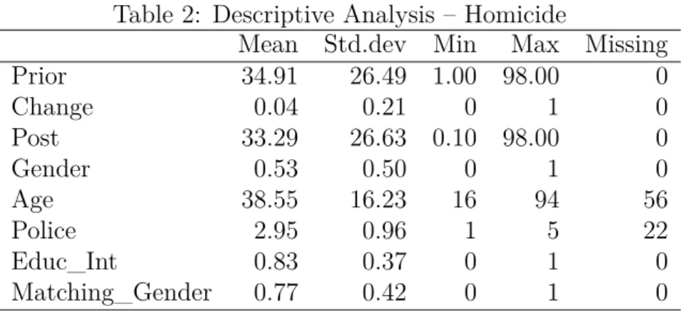
Table (2) summarizes the first sample statistics. We have already anticipated com-ments on Gender and Age. However, our empirical exercise is also going to include en-vironmental and matching issues, as well as interviewers’s characteristics. We argue that our interaction outcomes rely not only on the respondent’s side, but also on the sender’s side and on common features between both of them. Since we are trying to model per-ceived information, we should consider message quality aspects and a first natural choice is the interviewers’ level of education. All of our 20 questioners, at least, completed high school studies and 80% of them are undergraduate students or graduates.
Table 2: Descriptive Analysis – Homicide
Mean Std.dev Min Max Missing Prior 34.91 26.49 1.00 98.00 0 Change 0.04 0.21 0 1 0 Post 33.29 26.63 0.10 98.00 0 Gender 0.53 0.50 0 1 0 Age 38.55 16.23 16 94 56 Police 2.95 0.96 1 5 22 Educ_Int 0.83 0.37 0 1 0 Matching_Gender 0.77 0.42 0 1 0
Source: Elaborated by the author.
Equally, sources of information noise are concerns to take into account. Note that differences among interviewers and interviewees possibly raise obstacles on information, and it works against an update. In this sense, an important concept to this analysis is known as Homophily. McPherson, Smith-Lovin & Cook (2001) defines it as the contact between similar people occurring at a higher rate than among dissimilar people. It is important to keep in mind that, at first, homophily can be related to race, gender, age, religion, social status or any other similar characteristic relating individuals. For example, whenever a group exhibits one of these heterogeneities at a higher rate than it would be found randomly, there is homophily.
The impact of these differences on spontaneous groups’ formation and networks ties is widely documented since the early 1920’s. For example, Bott (1928) noted that school children formed friendships and play groups at higher rates if they were similar on de-mographic characteristics. The implications of homophily to information diffusion is a research agenda of recent papers such as Jackson (2009) and Golub & Jackson (2012). Both studies attest that, if a society is divided into several groups with a strong homophily within each one of them, i.e. contundent differences among groups, the convergence speed in which information spreads is decreased.
a particular heterogeneity between interviewers and interviewees. We conjecture that, in Latin cultures, gender plays a significant role on information credibility/use. Hence,
Matching_Gender was created to control this issue. In addition, given our interest in
vic-timization risk perception, the way respondents evaluate police forces is a very important piece of information to control for. In a range of five levels, individuals rated the police work around its middle point, which stands for Fare.
Finally, our subjective probabilities, i.e. Prior and Post, take almost the full range [0,100] with a huge variance. This initial result piles up to the empirical evidence
pre-sented in Manski (2004), refuting usual concerns about subjective probabilities being reported in values around 50%. Also, as in Delavande, Giné & McKenzie (2011), we re-fute the fears that poor, illiterate individuals in developing countries do not understand probability concepts. Equally, the significant difference between respondents’s initial per-ceptions and the official rate could be another source of distrust in such data type. Nev-ertheless, it finds reverberation in previous papers such as Dominitz & Manski (1996b) and Jr, Grasmick et al. (1999) also attesting the existence of a crime overestimation.
The fact is: although a high discrepancy between subjective victimization probabilities and official rates is not new, our participants were informed about the “true” probability and still less than 5% of them changed initial perceptions. Actually, following Hoffrage et al. (2000), we presented the same information in numbers (37 in 100.000), which brings better results in the participants’s use of probabilities. Therefore, given that initial perceptions are so overrated, what could explain almost no change in responses?
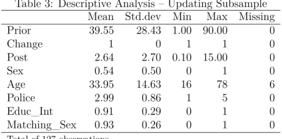
Perhaps looking at our updaters only provides some insight on this issue. It is impor-tant to keep in mind that we have two different steps after individuals receive an infor-mational shock: i) Whether or not to change initial responses; ii) Given that a change is going to happen, to what value it is going to be set. In a sample of 2885 responders, 2758 of them say no to the first question and 127 behave accordingly to previous studies on Bayesian updating processes. Since we have a reasonable updating subsample size here, we can restrict our analysis to this data part and look for any noticeable difference between updaters and the entire sample. Table (3) presents the results.
Table 3: Descriptive Analysis – Updating Subsample Mean Std.dev Min Max Missing Prior 39.55 28.43 1.00 90.00 0 Change 1 0 1 1 0 Post 2.64 2.70 0.10 15.00 0 Sex 0.54 0.50 0 1 0 Age 33.95 14.63 16 78 6 Police 2.99 0.86 1 5 0 Educ_Int 0.91 0.29 0 1 0 Matching_Sex 0.93 0.26 0 1 0
Total of 127 observations.
Source: Elaborated by the author.
into message quality might be on the right path. When we look back to table (2) and compare it with table (3), we find thatEduc_Int andMatching_Gender means increased considerably from 83% and 77% to 91% and 93%, respectively, in our updating subsample. Furthermore, Prior and Age are other variables that this crude analysis indicates to be aware of. The results show that our updaters are younger individuals with higher initial perceptions.
In summary, this very simple exercise induces us to believe that a selection bias might be working behind the scenes. Note that the Post reported is conditioned to a previous decision and, when we select our sample only for individuals who decide to change initial responses, this subgroup has some different characteristics from the entire sample. Those characteristics might be just what we are looking for.
Remember that our main purpose in this study is to investigate the role of hetero-geneity into the update of subjective homicide victimization risk after an informational shock. Guiding us to this task, Viscusi & O’Connor (1984) shows the existence of an estimable simple linear regression, using priors to explain posteriors. Also, Delavande (2008) provides us some insights on how to propose a Bayesian Update model allowing the possibility of skepticism, i.e. settingP rior =P ost.
In short, the data used here also attests the existence of a crime overestimation found in previous works. The novelty is that our respondents faced an informational shock consisting in the official homicide rate, but 95% of them keep the same initial perception. So far, looking at the updating subsample only, we found that these updating interactions were made by more educated interviewers, sharing the same gender with our interviewees. Thus, those two most important results enable us to follow our main line of explanation: informational quality.
4
ECONOMETRIC MODELS FOR BAYESIAN
UP-DATING
4.1
Classical Bayesian Update
As mentioned in subsection (2.1), the starting point of the Bayesian Theory is given by equation:
P(Hypothesis|Evidence)∝P(Evidence|Hypothesis)P(Hypothesis)
As a first motivating empirical exercise, consider the case of a random experiment composed by three coin tossesiid. Success, y= 1, consists of getting a head, with no loss
of generality and let θ be the unknown success probability. We want to use the tosses
result, say R= (1,0,1), to infer about the true value of θ.
The parameter θ is treated as an unknown parameter about which the individual has
a first approximation. Then, he will use evidence R to make an update over the true
value. Formally,
p(θ|R)∝p(R|θ)p(θ) (4)
wherep represents the probability distribution function at a Bayesian context.
Given the structure proposed,
p(R|θ) = θ2(1−θ) (5)
As for the heart of a Bayesian approach, we must admit an initial probability distribu-tion forθ. It represents the observer uncertainty about the population value. Following
Pratt, Raiffa & Schlaifer (1995) in the choice of aBetadistribution forBernoulliprocesses, we assume thatθ ∼Beta(α, β), i.e.,
p(θ) = Γ(α+β)
Γ(α)Γ(β)θ
α−1(1−θ)β−1 (6)
Substituting (5) and (6) into (4),
p(θ|R)∝θ2(1−θ)Γ(α+β)
Γ(α)Γ(β)θ
α−1(1−θ)β−1
i.e.,
p(θ|R)∝θα+1Γ(α+β)
Γ(α)Γ(β)(1−θ)
β (7)
Then, θ|R ∼ Beta(α+ 2, β+ 1). For the predicting exercise of y = 1 given R, we need p(y= 1|R). So,
p(x= 1|R) =
Z
p(y= 1, θ|R)dθ
=Z p(x= 1|θ, R)p(θ|R)dθ
=Z θp(θ|R)dθ
Then, the probability of getting a head in the next toss, given the past evidence, is:
P(y= 1|R) = p(y = 1|R) = E(θ|R)
Therefore,
P(y= 1|R) = α+ 2
(α+ 2) + (β+ 1)
Generalizing the number of tosses,
θ|(R1, R2, ..., RN)∼Beta(α+
N
X
i=1
Ri, β+N − N
X
i=1
Ri)
P(y= 1|(R1, R2, ..., RN)) =
α+PNi=1Ri
(α+PNi=1Ri) + (β+N − PN
i=1Ri)
Using this same reasoning, we will start our victimization expectation modeling. The
P rior collection is very similar to what we did here, but we introduce heterogeneity in
the discussion. Then, we look a bit closer to the role of observable and unobservable characteristics into the updating process, providing the first structural model. Finally, in assuming a linear form for the updating function, we propose our first estimable multiple linear model.
4.2
Multiple Linear Regression and Victimization Expectation
Update
Consider a victimization event, where y = 1 if the individual becomes a crime victim
and y = 0 on the contrary. Let Y ∼ Bern(π), iid, and assume that the respondent
has a probability distribution Beta(α, β) about the true, but unknown, probability π of
becoming a homicide victim.
In this fashion, we propose the following interaction structure: the initial respondent’s perception, P riori ≡ πi0, can be modeled as dependent on his observable characteristics,
for instance, age, gender, income, education, etc. Formally, we can define a function
f : Rq → [0,1] such that π0
i = f( ˜Xri), where ˜Xri is the q dimensional heterogeneity
vector of individual i. When asked about his initial perception, the individual assess P(y= 1|X˜ri) =E(π|X˜ri) =π0
i and establishes as response πi0 = αi
αi+βi.
After collecting π0
i, the interviewer sends an informational bit consisting in the
pop-ulation value, π. However, from the respondent’s perspective, this information may lack
credibility and its content may not be fully taken into account. In fact, letπ∗
i be the proper
value depicted by this information and defineg :Rk→[0,1], withπ∗
i =g(Xri,Xsj,Xmi,j, πi0).
In this function,Xr
i andXsj represent the vectors of observable heterogeneity for receivers9
and senders, respectively, andXm
i,j is a vector of matching aspects.
Abstractly, the information was translated into a sequence of victimization observa-tions, generating an informational contentI = (0,1, . . . ,0,1) withn1 values equal 1 and
n0 equal 0, where N =n0+n1. Finally, the respondent, whose initial perception wasπi0,
uses the perceived information,πi∗, to generateIi, creating a set of new evidence which is
the foundation to update his response towards a posterior perception. This new response,
P ost≡πip, is given by Pi(y= 1|Ii) = E(π|Ii) =πip.
9
In this structure,
pi(π|Ii)∝pi(Ii|π)pi(π)
∝πn1(1−π)n0Γ(αi+βi)
Γ(αi)Γ(βi)π αi−1(1
−π)βi−1
Then,
π|Ii ∼Beta(αi+n1, βi+n0)
And,
πpi =E(π|Ii) =
αi+n1
αi+βi+n1+n0
For estimation purposes,πip remains undefined, since it is not possible to identify none
of the given parameters. One way to dodge this problem is to realize that π∗
i = nN1 and
use the fact that π0
i = αi
αi+βi to establish:
πpi = N(n1
N) + (αi+βi) αi
(αi+βi)
αi+βi+N
Therefore, we are able to write our structural model as:
πip =
N
αi+βi +Nπ
∗ + αi+βi
αi+βi+Nπ
0
i (8)
Now, if we assume thatg :Rk →[0,1] is given by a linear form, it allows us to extend
Viscusi & O’Connor (1984) and Smith & Johnson (1988) at the same time by taking not only respondent’s heterogeneity into account, but also both interviewer and matching information through a coherent conditioning multiple linear regression as follows::
πpi =λ+γπi0+Xiδ+ǫ (9)
whereXi is an extended vector composed by Xri,Xsi,Xmi .
4.3
Bayesian Updating with Skepticism
As explored in section (3), we have a very different sample in the context of Bayesian Update. Our data presents an excess of individuals – our skeptical agents – who do not update and keep their posterior responses with the same value as their initial perceptions, i.e. P riori =P osti. One might point this issue as an important downside of our study.
In fact, previous works present data collection procedures specifically designed to assess subjective probabilities and its revision processes10. On the other hand, our dataset comes
from a broad household survey.
Clearly, individuals faced a critical question – homicide expectation – about which initial perceptions were too far from the truth. In addition, the information provided lasted less than a couple of minutes. However, even under such circumstances, if we proceed the estimation of equation (9) considering only those 127 individuals who changed initial responses, we will work on a sample almost 40% greater than what is presented in Delavande (2008), for example. Indeed, this exercise is part of our estimation procedure presented in subsection (4.3.2).
10
By now, we want to extend the discussion on informational content raised by Viscusi & O’Connor (1984) to move from an extreme, where almost every participant revises their initial perception, to the other, where the contrary occurs. Is that reasonable to keep considering an economy composed by agents who always believe in the information received for every risky decision to be made? Putting in other words, is all information provided about uncertain outcomes informative enough to make almost every individual change initial perceptions? Our dataset sends a clear message: for victimization expecta-tions this is not the case and restricting attention only to those updaters would lead us, at least, to waste a huge amount of information. Also, these statistics reported might be misleading, due to potential selection bias.
In this study, it is important not to neglect individuals who did not respond to new information, since they carry messages about the updating process. Still, how to accom-modate rational individuals in the same model facing the same information but behaving so differently? At this point, it is clear for us that our venture and major contribution is to propose a framework compatible to a Bayesian Update allowing the possibility that no update takes place. The main question is: could we build an econometric model which was able to estimate the impact of P riori on P osti and, at the same time, consider the
fact thatP riori is a threshold point for the existence of an update? In this sense, we seek
to develop an econometric model which is able to address the following issues:
i) Agents are Bayesian when updating their victimization expectations;
ii) Observable and non-observable heterogeneity must refer not only to the interviewee but also to the interviewer, since matching aspects may influence credibility and information usage;
iii) The presence of non updating individuals must receive an adequate treatment and be rationalized under a Bayesian context.
With that in mind, rewrite (8) as follows:
πpi =
1 + αi+βi
N
−1
π∗+1 + N
αi+βi
−1
π0i (10)
Note that, fromπi0, we may interpretαi+βi as the quantity of samples initially used
to form P riori. Following this reasoning, ηi = N
αi+βi ∈ [0,∞) may be interpreted as a
measure of the informational quality. In this way, (10) can be rewritten as:
πpi =
1 + 1
ηi
−1
π∗+1 +ηi−1πi0 (11)
This structural form will be crucial to skepticism rationalization. We need to explain individuals setting πpi = πi0, and it is reasonable to assume that the decision to revise
perceptions, i.e to make πip 6= π0
i, is directly related to the credibility and quality of
the information obtained. As (11) makes clear, when ηi approaches zero, or the more
irrelevant the information is seen by the decision maker,πip approaches πi0, which, in the
limit, translates into the complete non-existence of an update. In the other extreme, when
ηi approaches the infinity, πpi takes exactly the value πi∗.
In summary, individuals setting P osti = P riori tell us that informational content
rational decision based on an intrinsic optimization process, which might be dependent on observable characteristics. Therefore, technically, there are observable and unobservable characteristics influencing a previous decision, subsetting our sample non-randomly.
In this situation, as pointed out by Wooldridge (2010), it is hard to believe that the now restricted error term has a zero conditional mean and, even if the structural model is linear, OLS procedure leads to inconsistent parameter estimates. The appropriate approach to deal with these cases is to think of an unrestricted and unobservable latent
variable underlining the true observations through a specific structure. That is exactly what we will develop next.
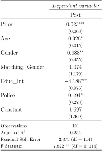
4.3.1 Model 1: A Generalized Tobit for Bayesian Updating
Initially, let Y be a random variable of interest and Y∗ its latent counterpart. then,
Yi∗ =Xiδ+ui, ui|Xi ∼N ormal(0, σ2) Yi =max(0, Yi∗)
whereXi is a vector of conditioning variables.
This model, originally motivated by Tobin (1958), is known as theStandard Censored
Tobit Model. Adapting it for our purposes, we assume the existence of a latent variable
P ost∗
i that will govern the censoring mechanism. What is P ost∗i? We conjecture that P ost∗
i captures the respondents’ latent posterior probability and, as such, according to
equation (9), we propose it is a function of theprior and of an observable variables vector regarding both interviewees and interviewers. Hence, consider the following Tobit:
P ost∗i =γP riori+Xiδ+ui, ui|P riori,Xi ∼N ormal(0, σu2) (12a)
P osti = min(P riori, P ost∗i) (12b)
But why the minimum? This is so because, in our sample, all initial perceptions are greater than the official rate. Thus, for the sake of rationality, we must have P osti ≤ P riori ∀i. Now, note that:
P osti = min(P riori, P ost∗i) =−max(−P riori,−P ost∗i)
However,
max(−P riori,−P ost∗i) = max(0, P riori−P ost
∗
i)−P riori
Then,
P osti =P riori−max(0, P riori−P ost∗i)
This means that our Tobit is equivalent to the following “new” Tobit:
P riori−P ost∗i = (1−γ)P riori−Xiδ+vi (13a)
P riori−P osti = max(0, P riori−P ost∗i) (13b)