ISSN 0101-8205 www.scielo.br/cam
A regularized solution with weighted
Bregman distances for the inverse problem of
photoacoustic spectroscopy
A.J. SILVA NETO and N. CELLA
Instituto Politécnico, IPRJ, Universidade do Estado do Rio de Janeiro, UERJ P.O. Box 97282, 28601-970 Nova Friburgo, RJ, Brazil
E-mails: [email protected] / [email protected]
Abstract. In the present work we propose the use of weighted Bregman distances in the
construction of regularization terms for the Tikhonov functional applied for the formulation and
solution of the inverse problem of photoacoustic spectroscopy. Test case results demonstrate
that better estimates were obtained for the simultaneous estimation of the thermal diffusivity and
optical absorption coefficient using, as synthetic experimental data, the information on both the
amplitude and phase-lag of the temperature at the interface sample-gas between the material under
analysis and the air chamber of the closed photoacoustic cell.
Mathematical subject classification: 35K05, 80A23, 90C30.
Key words: inverse problems, Tikhonov’s regularization terms, Bregman distances,
photo-acoustic spectroscopy, optical properties, thermal properties.
1 Introduction
The Photoacoustic Spectroscopy (PAS) [1], or more generally the Photothermal Spectroscopy [2–4], are non-destructive testing methodologies that have been applied for the thermal and optical characterization of materials [5–16]. There are other applications under development, such as gases monitoring [17, 18] and investigation of thermal contact resistance for copper coatings on carbon surfaces [19].
The photoacoustic effect is the basic phenomenon upon which PAS is built, and it occurs when a material sample placed inside a closed cell filled with air is illuminated with periodically interrupted light. The light absorbed by the sample is converted into heat through a nonradiative de-excitation process. The periodic flow of heat into the air chamber of the cell produces, as an acoustic piston, pressure disturbances in it, which can be detected by a microphone mounted at the cell wall. In the model for the direct problem developed by Rosencwaig and Gersho [20], known as RG theory, this is the only phenomenon taken into account in the PAS signal.
The PAS inverse problem is known to be ill-conditioned, and therefore regu-larization methods are usually required for its solution.
A number of different authors have investigated this problem, see for example Refs. [21–26], and most of them use Tikhonov’s regularization. Such approach allows the use of a priori information, when available.
In a previous work [27] we used an implicit inverse problem formulation, and the Levenberg-Marquardt method, for the PAS with the direct problem modeled with the RG theory. As experimental data it was used only the amplitude of the steady periodic temperature established at the surface of the material sample that is next to the air chamber of the closed photoacoustic cell. We were able to estimate, separately, the thermal diffusivity,α, the thermal conductivity, k, and the optical absorption coefficient,β, of the material under analysis. However, it was not possible to estimate any pair of coefficients simultaneously.
were, respectively, of the order of 14% and 7%. The range of the modulated frequency for external illumination was shifted from 5-17 Hz (in [27]) to 1-8 Hz (in [28]) in order to have a higher sensitivity of the parameters to be estimated.
In both works [27, 28], it was required, for most of the test cases, the use of a damping factor in the Levenberg-Marquardt method in order to achieve convergence.
As mentioned before, Tikhonov’s regularization [29] is the most well known approach used for the solution of ill-posed problems. In order to deal with the effects of the noise present in the experimental data, it has been used in numerous different areas of application [30–34].
Much work has been done on the analysis and proposition of regularization terms for Tikhonov’s functional [35–39], and the proper choice of the regulariza-tion parameter is of key importance for the implementaregulariza-tion of such an approach for the solution of inverse problems [40–42].
Cidade et al. [43, 44] proposed the use of Bregman distances [45] as Tikhonov’s regularization terms for one application in the restoration of atomic force mi-croscopy nanoscale images. Using Csiszár’s measure [46], called q-discrepancy, a family of regularization terms was constructed. Berrocal Tito et al. [47] and Pinheiro et al. [48] extended this idea by using moments of the q-discrepancy. The former work [47] is related to the estimation of parameters in an environ-mental model, and the latter [48] deals with an inverse problem of radiative properties estimation.
In the present work a one parameter family of regularization terms constructed with Bregman distances based on the q-discrepancy function is implemented in the formulation and solution of PAS as an inverse problem. The original idea [43, 44] was improved by the proper weighting of the unknowns to be determined, and we use here the denomination weighted Bregman distances. We have focused on the simultaneous estimation of the sample thermal diffusiv-ity,αs, and optical absorption coefficient,β.
The effects of the parameter q used in the construction of the regularization terms, as well as those of the regularization parameterλare investigated. Some test case results are presented.
As real experimental data is not yet available, we have used synthetic exper-imental data. The experexper-imental apparatus is available at our institution, and in the near future we will be able to acquire real experimental data. Before dealing with the difficulties associated with the real experiments, we decided to perform the numerical simulations in order to evaluate the best conditions in which the experiments will be performed.
2 Mathematical formulation and solution of the direct problem – RG theory
Consider the cylindrical closed photoacoustic cell represented schematically in Figure 1. The sample of the material under analysis is placed upon a backing material, and the other boundary of the sample adjoint to the air chamber of the cell, is exposed to an incident modulated light with intensity
I(t)= 1
2I0[1+cos(ω∙t)] (1)
where I0is the maximum intensity of the incident light,ωis the angular frequency of the chopping mechanism, and t represents time.
It is assumed that the light doesn’t go through any interaction within the air chamber and is fully absorbed by the material sample according to Beer’s law
Is(x,t)=eβxI(t) (2)
whereβ is the optical absorption coefficient, the subscript s represents the sam-ple, and x is the space coordinate representing the depth in the sample starting at the interface between the sample and the air chamber, as shown in Figure 1.
The volumetric heat generation at the sample due to the light absorbed is given by
S(x,t)= d Is(x,t)
d x =
1 2βI0e
Figure 1 – Schematical representation of the closed photoacoustic cell.
and the mathematical formulation of the heat conduction problem in the photoa-coustic cell is given by
∂2θg(x,t) ∂x2 =
1 αg
∂θg(x,t)
∂t , 0<x <lg (4a)
∂2θs(x,t) ∂x2 =
1 αs
∂θs(x,t) ∂t −
βI0 2kse
βx 1
+ejωt
, −ls <x <0 (4b)
∂2θb(x,t) ∂x2 =
1 αb
∂θb(x,t)
∂t , −(lb+ls) <x <−ls (4c)
with the interface conditions given by
θs(0,t)=θg(0,t) , θs(−ls,t)=θb(−ls,t) (4d, e)
ks
∂θs(x,t) ∂x
x=0
= kg
∂θg(x,t) ∂x
x=0
(4f)
ks
∂θs(x,t) ∂x
x=−ls
=kb
∂θb(x,t) ∂x
x=−ls
and the initial conditions given by
θg(x,0)=0, 0≤ x ≤lg (4h)
θs(x,0)=0, −ls ≤x ≤0 (4i)
θb(x,0)=0, −(ls +lb)≤x ≤ −ls (4j)
where j is the imaginary number√−1,θ is the complex valued temperature, k represents the thermal conductivity,αthe thermal diffusivity, and the subscripts
g,s and b denote air (gas), sample and backing material, respectively.
The complete solution for problem (4) is given in [1, 20, 27]. Here we are interested only in the temperature at the sample-gas interface, i.e. x=0,
θ (0,t)=F0+θ0ejωt (5) where F0is the time-independent (dc) component of the solution at x =0, and θ0is a complex valued number given by
θ0=
p1−p2+ p3
p4−p5
H, p1=(r −1) (b+1)eσsls, (6a, b)
p2=(r+1) (b−1)e−σsls, p3=2(b−r)e−βls, (6c, d)
p4=(g+1) (b+1)eσsls , p5=(g−1) (b−1)eσsls, (6e, f)
H = βI0
2ks(β2−σ2 s)
, b= kbab
ksas
(6g, h)
g= kgag ksas
, r = (1− j)β
2as (6i, j)
as =
ω 2αs
12
, ab =
ω 2αb
12
(6k, l)
ag=
ω 2αg
12
, σs =(1+ j)as (6m, n)
part is of physical interest. Therefore, we choose only the terms
Re [θ (0,t)]ac = |θ0|cos(ωt+φ) (7) Writing,
θ0=θ1+ jθ2 and θ1=Re [θ0], (8)
θ2 =Im [θ0] and θ0= |θ0|ejφ (9)
we obtain the amplitude
A= |θ0| =
q
θ2
1 +θ22 (10)
and the phase-lag
φ =arctan
θ2 θ1
(11)
If we know the optical and thermal properties of the sample, the thermal prop-erties of the other materials in the photoacoustic cell, the physical dimensions
ls, lband lgrepresented in Figure 1, the frequency of the chopping mechanism, and the intensity of the incident light, then eqns. (10) and (11) provide the calcu-lated values for the amplitude and phase-lag of the temperature at the interface sample-gas between the material and the air chamber at x =0.
3 Mathematical formulation and solution of the inverse problem
Consider a vector of unknowns,
E
Z =
Z1,Z2, ...,ZNu
T
(12)
where Zi,i =1,2, . . . ,Nu, are thermal or optical properties of a sample of the material being tested by Photoacoustic Spectroscopy (PAS), and Nu represents the total number of unknowns.
For each modulation frequency used in the PAS experiment, i.e. fi, i = 1,2, . . . ,Nf, where fi = ωi
The inverse problem is then formulated as an optimization problem in which we seek to minimize Tikhonov’s regularization functional
TZE =
2Nf
X
i=1
h
Ci
E
Z−Ei
i2
+λSZE,ZER
= ERTRE+λS
E
Z,ZER
(13)
where Ci(ZE) and Ei represent the calculated and experimental values of the amplitude, for i =1,2, . . . ,Nf, and the calculated and experimental values of the phase-lag, for i = Nf +1,Nf +2, . . . ,2Nf, R is the vector of residuesE given by
E
R=
Acalc1 −Aexp1, . . . ,AcalcN f −AexpN f,
φcalc1 −φexp1, . . . , φcalcN f −φexpN f
T (14)
λis the regularization parameter, S represents the regularization terms, andZER is a vector of reference values for the unknowns we want to determine, Z . WeE
have made an adjustment by a constant factor in the calculated and experimental values for the amplitudes, Aexpi and Acalci,i = 1,2, . . . ,Nf, to make them of
the same order of magnitude as the phase-lag values.
Using Csiszár’s measure [46], here called q-discrepancy [43, 44], we have
ηq E Z = 1
1+q
Nu
X
i=1
Zi
Zqi −mq
q (15)
where q is a real valued number with q>0, and m is a measure associated with a prior information (it will cancel out in the calculations to be done next), and the Bregman distance [43–45]
Dq
E
Z,ZER
=ηq
E
Z
−ηq
E
ZR
−D∇ηq
E
ZR
,ZE − EZR
E
(16)
a family of one parameter regularization terms can be constructed. From eqns. (15) and (16), we obtain
Dq
E
Z,ZER
= 1
1+q
Nu
X
i=1
(
Zi
Ziq− ZiR
q
q − Z
R i
q
Zi−ZiR
)
We must stress that varying the parameter q, with q >0, a family of regular-ization terms is obtained.
By taking the limit q → 0 in eqn. (17a), one gets the cross-entropy regular-ization term
D0
E
Z,ZER
=
Nu
X
i=1
Ziln
Zi
ZR i
− Zi −ZiR
(17b)
and with q=1 the usual energy regularization term is derived, namely
D1
E
Z,ZER
= 1
2 Nu
X
i=1
Zi −ZiR
2
(17c)
As the unknowns Zi,i =1,2, . . . ,Nu, may be of different orders of magni-tude, we propose a modification to eqn. (17a) by introducing a weighting factor 1
fZi,i =1,2, . . . ,Nu, such that
ˉ
Dq
E
Z,ZER= 1
1+q
Nu
X
i=1 1
fZi
(
Zi
Ziq− ZiR
q
q − Z
R i
q
Zi−ZiR
) (18a) ˉ Dq E
Z,ZERdenominated weighted Bregman distances, for the particular case of q→0 results in
ˉ
D0
E
Z,ZER
=
Nu
X
i=1 1
fZi
Ziln
Zi
ZR i
− Zi −ZiR
(18b)
In the present work we consider the weighting factor
fZi = Z
R i
q+1
, i =1,2, ...,Nu (19)
The regularization term in eqn. (13) may then be either
S
E
Z,ZER
= Dq
E
Z,ZER
or S
E
Z,ZER
= ˉDq
E
Z,ZER
(20a, b)
As described in [43, 44] the use of Bregman distances constructed with the
q-discrepancy measure yields a one-parameter family of regularization terms in
are particular cases. See eqns. (17b) and (17c). Therefore, by simply varying one parameter, q, different solutions are obtained and the user may decide which one is the best for a given application. It must be stressed that different sets of experimental data with different levels of noise are better handled by different regularization terms [43, 44, 49].
It is important to mention also that the regularization terms given by eqns. (20a,b) allow the use of prior information on the unknowns by including refer-ence values for such parameters.
In order to minimize the cost function given by eqn. (13), we write the critical point equation as
∂T
E
Z
∂ZE =0 i.e.
∂T
E
Z
∂Zj =
0, j =1,2, . . . ,Nu (21a, b)
resulting
JTRE+λSEZE =0 (22)
where the elements of the Jacobian matrix J are given by
Jst = ∂Cs ∂Zt
, s=1,2, . . . ,2Nf and t =1,2, . . . ,Nu (23)
and
E
SZE =
∂S
∂Z1 , ∂S
∂Z2
, . . . , ∂S ∂ZNu
T
(24)
The elements of the Jacobian matrix J , given by eqn. (23), were calculated numerically by using a central finite-difference approximation. By using the Taylor’s expansions
E
R
E
Zn+1
= ER
E
Zn
+Jn1ZEn (25)
E
SZ
E
Zn+1= ESZEZEn+JSn1ZEn (26) where n is used as the iteration index in the iterative procedure that will be constructed for the estimation of the vector of unknownsZ ,E
E
and the elements of the Jacobian matrix Js are given by
JSuv =
∂SZu
∂Zv = ∂ ∂Zv
∂S
∂Zu
, u=1,2, . . . ,Nu andv=1,2, . . .Nu (28)
Introducing eqns. (25) and (26) into eqn. (22) results in the following:
JnTJn+λJSn
1ZEn= −JnTREn+λSEZnE
(29) We are now in a position to construct an iterative procedure for the estimation of the vector of unknownsZ . We first choose an initial guessE ZE0, which may be for example,
E
Z0= EZR (30)
and then we calculate the Jacobian matrices J0 and J0
S, whose elements are given by eqns. (23) and (28), respectively, as well as the elements of the vector of residues given by eqn. (14). Next, the vector of corrections1ZE0 is calcu-lated by solving the system of algebraic linear equations (29). The vector, with new estimates for the unknowns, ZE1, is obtained using eqn. (27). The iterative procedure for calculating the corrections1ZEnwith eqn. (29) and new estimates for the unknownsZEn+1with eqn. (27) is continued until a convergence criterion
such as
1Zi
Zi
< ε for i =1,2, . . . ,Nu (31)
is satisfied, whereεis a given tolerance.
Before we proceed, we must show how the elements of the vectorSEZE, and the
elements of the Jacobian matrix JS, are calculated. From eqns. (20a,b) and (24) we observe that
∂S
∂Zj = ∂Dq ∂Zj
, j=1,2, . . . ,Nu or (32a)
∂S
∂Zj = ∂Dˉq ∂Zj
, j=1,2, . . . ,Nu (32b)
and from eqns. (28) and (32a,b) we obtain
JSuv =
∂2D q ∂Z2
u
if u =v
0 if u 6=v
or
JSuv =
∂2Dˉq ∂Z2
u
if u =v
0 if u6=v
u =1,2, . . . ,Nuandv=1,2, . . . ,Nu (33b)
The first and second derivatives of the Bregman distance in eqns. (32a,b) and (33a,b) are obtained from eqns. (17a,b) or (18a,b). These derivatives, as well as the Bregman distances, are shown in Table 1 for both situations: (a) regular Bregman distances, and (b) weighted Bregman distances.
(a) regular (b) weighted
Dq=1+1q Nu X i=1
ZiZi q−Z Rq
i
q −Z R
q
i
Zi−Z Ri ˉ Dq=1+1q
Nu X i=1
1
f Zi ZiZi q−Z Rq
i
q −Z R
q i
Zi−Z Ri
D0=NuP i=1
( Zi ln Zi
Z Ri !
−Zi−Z R i
)
ˉ D0=NuP
i=1 1
f Zi (
Zi ln Zi Z Ri !
−Zi−Z R i
)
∂Dq
∂Z j =
Zqj−Z R q
j
q , j=1,2, ...,Nu
∂Dqˉ
∂Z j = 1
f Zj Zqj−Z R
q
j
q , j=1,2, ...,Nu
∂D0 ∂Z j =ln
Z j Z Rj
, j=1,2, ...,Nu
∂D0ˉ ∂Z j=
1
f Zj
ln
Z j Z Rj
, j=1,2, ...,Nu
∂2 Dq ∂Z 2
j
=Zqj−1, j=1,2, ...,Nu ∂
2Dqˉ
∂Z 2 j
= 1 f Zi Z
q−1
j , j=1,2, ...,Nu
∂2 D0 ∂Z 2j =
1
Z j, j=1,2, ...,Nu
∂2D0ˉ ∂Z 2j =
1
f Zi
1
Z j, j=1,2, ...,Nu
Table 1 – Bregman distances used as regularization terms, and the first and second derivatives for both cases: (a) regular Bregman distances, and (b) weighted Bregman distances.
4 Results and discussion
generated with
Ei =Ci
E
Zexact
+2.576 riσ, i =1,2, . . . ,2Nf (34)
where ri is a random number in the range [-1,1], andσ represents the standard deviation of the measurement errors. The level of noise in the experimental data that will be reported next for the numerical test cases is computed by
noi sei(%)=
2.576 riσ
Ci
×
100%, i=1,2, . . . ,2Nf (35)
and we take the maximum value of the noi sei(%),i =1,2, . . . ,2Nf.
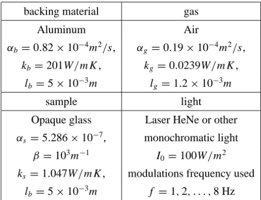
In order to compare the performance of the approach developed in the present work with that presented in [27, 28], we used the same geometry, process, ther-mal and optical parameters for the photoacoustic cell and for the sample of the material under analysis. In the test cases performed we have used frequencies of the modulated incident light from 1 to 8 Hz, which may yield higher sensitivities to the parameters we want to determine [28]. In Table 2 is presented a summary of the process, thermal and optical parameters used.
backing material gas
Aluminum Air
αb=0.82×10⁻⁴m2/s, αg =0.19×10⁻⁴m2/s,
kb=201W/m K , kg=0.0239W/m K ,
lb=5×10⁻³m lg=1.2×10⁻³m
sample light
Opaque glass Laser HeNe or other
αs =5.286×10⁻⁷, monochromatic light β =103m−1 I
0=100W/m2
ks =1.047W/m K , modulations frequency used
lb=5×10⁻³m f =1,2, . . . ,8 Hz
using three approaches: (i) without regularization, (ii) with regularization using the regular Bregman distances, and (iii) with regularization using weighted Breg-man distances. The first approach corresponds toλ=0 in eqn. (13), and for the second and third approachesλ=0.03 and q =1 with the regularization terms given, respectively, by eqns. (20a) and (20b). The reference values and the ini-tial estimates for the thermal diffusivity and optical absorption coefficients were taken as: αsR =4.0×10⁻⁷m2/s,βR =9.5×10²m−1,αs0 =5.0×10⁻⁶m2/s,
andβ0=0.9×10³m−1. The exact values, which we want to recover, are shown in Table 2.
Five computations were performed for each approach, using for each computa-tion a different set of pseudo-random numbers, simulating therefore five different experiments. The value ofσ = 0.5 in eqn. (34) led to synthetic experimental data with noise up to 4%.
Convergence difficulties were observed when the initial guesses were not taken close enough to the exact values, as usually happens with Newton-type methods. Therefore, in order to achieve convergence the full Newton correction step in eqn. (27) was not used. Instead we have applied a gain factorγ, with 0≤γ ≤1, such that
E
Zn+1= EZn+γ 1ZEn (36)
To obtain the results presented in Figure 2 we usedγ =0.5.
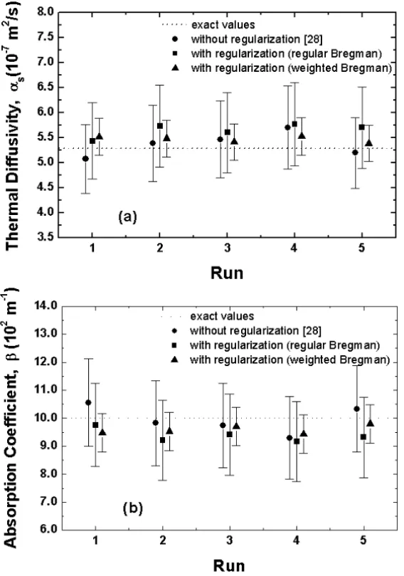
From Figure 2 we may conclude that the use of the regularization terms with weighted Bregman distances yielded better results, i.e. smaller confidence bounds. Nonetheless we must be careful because the confidence bounds were calculated using the inverse of the matrix JTJ+λJS, and therefore higher val-ues ofλcould yield smaller confidence bounds. This subject deserves further investigation.
Figure 2 – Estimates and confidence bounds for (a) thermal diffusivity, and (b) optical absorption coefficient using three approaches: without regularization; with regulariza-tion using regular Bregman distances; and with regularizaregulariza-tion using weighted Bregman distances.
therefore usedγ =1 in eqn. (36), going back to eqn. (27). It was also observed that the use of two different initial guesses led to very similar estimates for the unknowns, i.e. within the same order of confidence bounds and deviation of the exact values.
From the results shown in Figure 3a we observe a reduction in the values of the confidence bounds when the regularization with the weighted Bregman distances is used, but as mentioned before this reduction may have been caused by the terms added to the diagonal of the information matrix.
From the results presented in Figure 3b, for the difference between the esti-mated and exact values for the unknowns, we obtain as average values for 10 runs 4.33±2.84% and 4.86±3.07% for the thermal diffusivity, α, and the optical absorption coefficient,β, respectively, when no regularization is used. With the weighted Bregman regularization the following values are obtained: 2.97 ±1.42% and 3.60±1.72%. Therefore, one observes that not only the differences forα andβ are reduced when regularization is used, but also the standard deviation computed using 10 runs of the algorithm. This behavior is also observed in the results presented in Figure 4 and Table 3.
In Figure 4 are presented the variation of the average for the confidence bounds as a percentage of the estimated values of the unknowns, and the variation of the average values of the differences between the estimated and exact values, with the regularization parameterλand with the parameter q.
Here we have consideredα0s = αsR = 4.0×10⁻⁷m2/s, β0 = βR = 9.5×
102m−1, and the exact values of the unknown parameters are given in Table 2. It must be stressed that in Figure 4 the error bars correspond to one standard deviation from the average values of both the percentage differences and confi-dence bounds (as a percentage of the estimated values) obtained in 10 runs for each value of q and for each value ofλ. The standard deviation was calculated from the distribution of the results obtained in the 10 runs. Further, from the observation of the error bars shown in Figure 4 we conclude that the deviation of the estimates forαandβbecome smaller as higher values ofλare considered for a given value of q.
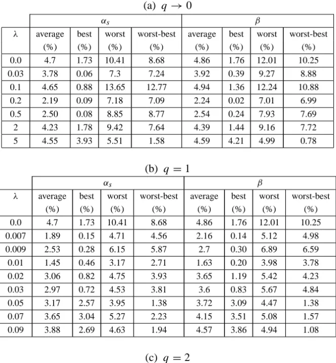
In Table 3 are presented the average, the best and the worst values for the differences between the estimated and exact values for the thermal diffusivityα and the optical absorption coefficientβ. In Table 3 is also presented the difference between the worst and the best values for the percentage differences.
(a) q →0
αs β
λ average best worst worst-best average best worst worst-best
(%) (%) (%) (%) (%) (%) (%) (%)
0.0 4.7 1.73 10.41 8.68 4.86 1.76 12.01 10.25
0.03 3.78 0.06 7.3 7.24 3.92 0.39 9.27 8.88
0.1 4.65 0.88 13.65 12.77 4.94 1.36 12.24 10.88
0.2 2.19 0.09 7.18 7.09 2.24 0.02 7.01 6.99
0.5 2.50 0.08 8.85 8.77 2.54 0.24 7.93 7.69
2 4.23 1.78 9.42 7.64 4.39 1.44 9.16 7.72
5 4.55 3.93 5.51 1.58 4.59 4.21 4.99 0.78
(b) q =1
αs β
λ average best worst worst-best average best worst worst-best
(%) (%) (%) (%) (%) (%) (%) (%)
0.0 4.7 1.73 10.41 8.68 4.86 1.76 12.01 10.25
0.007 1.89 0.15 4.71 4.56 2.16 0.14 5.12 4.98
0.009 2.53 0.28 6.15 5.87 2.7 0.30 6.89 6.59
0.01 1.45 0.46 3.17 2.71 1.63 0.20 3.98 3.78
0.02 3.06 0.82 4.75 3.93 3.65 1.19 5.42 4.23
0.03 2.97 0.72 4.53 3.81 3.6 0.83 5.67 4.84
0.05 3.17 2.57 3.95 1.38 3.72 3.09 4.47 1.38
0.07 3.65 3.04 5.27 2.23 4.15 3.51 5.08 1.57
0.09 3.88 2.69 4.63 1.94 4.57 3.86 4.94 1.08
(c) q =2
αs β
λ average best worst worst-best average best worst worst-best
(%) (%) (%) (%) (%) (%) (%) (%)
0.0 4.7 1.73 10.41 8.68 4.86 1.76 12.01 10.25
0.0001 5.22 0.88 8.7 7.82 5.33 0.91 8.71 7.8
0.0002 4.44 3.45 6.27 2.82 4.1 2.78 6.09 3.31
0.0005 4.98 3.66 6.01 2.35 4.92 3.65 5.90 2.25
0.0012 4.22 3.79 4.49 0.70 4.78 4.49 5.14 0.65
0.0020 5.28 4.75 5.94 1.19 4.93 4.51 5.48 0.97
regularization with the weighted Bregman distances.
From the results presented, we conclude that for different values of the pair (λ,q)the error in the estimates of the unknowns are of the order of, or smaller than, the level of the noise present in the experimental data, which represents an improvement on the results presented in [28].
It is interesting to observe that the spread of the estimates tends to become smaller when regularization is used. In Table 3 this corresponds to smaller values of the difference between the worst and the best estimates, i.e. worst-best in the fifth and ninth columns.
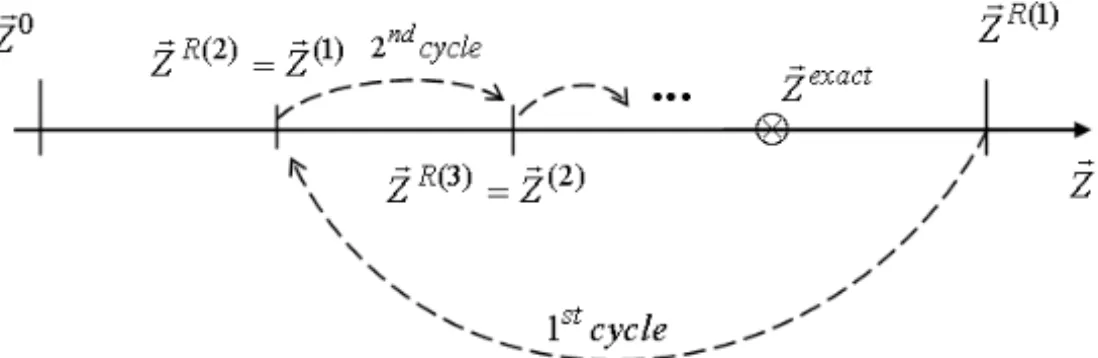
In order to get better estimates for the unknowns we have also implemented a feedback approach, following [50], in which the estimates at the end of one cycle of iterations, i , i.e. ZE(i), are used as the new values for the reference parameters in the subsequent cycle of iterations,ZER(i+1) = EZ(i). A schematical representation of the feedback approach is presented in Figure 5. Observe that the superscripts in parenthesis represent a specific cycle of iterations. As an example of the application of the feedback approach, we considered the pair λ = 0.05 and q = 1.0, and α0
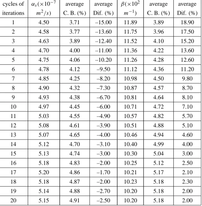
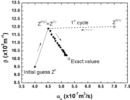
s = 4.0×10⁻⁷m2/s, β0 = 9.5×10²m−1, αsR(1) = 7.0×10⁻⁷m2/s, andβR(1) = 1.2×10³m−1. The exact values to be recovered are shown in Table 2. The results are presented in Table 4. Each result presented in Table 4 corresponds to an average calculated with five runs of the algorithm. The results shown in Table 4 are also presented graphically in Figure 6.
From the results presented in Table 4 and Figure 6 we observe the conver-gence ofα andβ to numerical values (average over the last 5 cycles of itera-tions)(5.17±0.02)×10−7m2/s and(10.22±0.02)×102m−1, respectively. Therefore, with this approach we were able to obtain better estimates than those obtained without the feedback approach whose results are shown in Figure 4b. In order to clarify this point such results are presented in Table 5.
cycles of αs(×10−7 average average β(×102 average average iterations m2/s) C. B. (%) Dif. (%) m−1) C. B. (%) Dif. (%)
1 4.50 3.71 –15.00 11.89 3.89 18.90
2 4.58 3.77 –13.60 11.75 3.96 17.50
3 4.63 3.89 –12.40 11.52 4.10 15.20
4 4.70 4.00 –11.00 11.36 4.22 13.60
5 4.75 4.06 –10.20 11.26 4.28 12.60
6 4.78 4.12 –9.50 11.12 4.36 11.20
7 4.85 4.25 –8.20 10.98 4.50 9.80
8 4.90 4.32 –7.30 10.87 4.57 8.70
9 4.93 4.38 –6.70 10.81 4.64 8.10
10 4.97 4.45 –6.00 10.71 4.72 7.10
11 5.03 4.55 –4.90 10.57 4.82 5.70
12 5.08 4.61 –3.90 10.51 4.88 5.10
13 5.07 4.65 –4.00 10.46 4.94 4.60
14 5.12 4.70 –3.10 10.40 4.99 4.00
15 5.13 4.74 –3.00 10.30 5.04 3.00
16 5.18 4.83 –2.00 10.25 5.12 2.50
17 5.20 4.86 –1.70 10.21 5.17 2.10
18 5.18 4.87 –2.00 10.23 5.18 2.30
19 5.14 4.88 –2.70 10.20 5.18 2.00
20 5.15 4.91 –2.50 10.20 5.18 2.00
Table 4 – Estimates obtained for the thermal diffusivity,αs, and the optical absorption coefficient, β, with the feedback approach using the weigthed Bregman distances as regularization terms withλ = 0.05 and q = 1.0, and αs0 = 4.0×10⁻⁷m2/s and
β0 =9.5×10²m−1. Also the reference values used at the first cycle of iterations are
αsR(1) = 7.0 ×10⁻⁷m2/s andβR(1) = 1.2×10³m−1. For the thermal diffusivity,
Figure 5 – Schematical representation of the feedback approach. The superscripts in parenthesis represent a specific cycle of iterations. ZE(i)represents the estimates obtained at the end of the cycle of iterations(i), and it is used as the reference value for the next cycle of iterations, i.e. ZER(i+1)= EZ(i). The initial guess isZE0, and it is kept the same throughout the iterative procedure.
αsesti mat ed−αsexact αexacts
×100%
βesti mat ed−βexact βexact
×100%
From Table 3(b)
q=1,λ=0.05
without the feedback 3.17±0.49 3.72±0.50
approach (average of
10 runs)
From Table 4
q=1,λ=0.05
with the feedback 2.18±0.41 2.18±0.22
approach (average
over the last 5 cycles
of iterations).
Table 5 – Comparison of the absolute values for the average of the difference between estimated and exact thermal diffusivity,α, and optical absorption coefficient,β, obtained with and without the feedback approach.
5 Conclusions
Figure 6 – Graphical representation of the results presented in Table 4 for the feedback approach. The level of noise in the synthetic experimental data was up to 4%. The numbers in parenthesis indicate the cycle of iteration and the dots represent the estimates obtained at the end of each cycle of iteration. ZE0is the initial guess and it is kept the same throughout the iterative procedure.
The use of weighted Bregman distances constructed with the q-discrepancy functional as regularization terms in Tikhonov’s functional appears to yield better estimates for the unknowns. We have varied both the regularization parameter λand the parameter q in the weighted Bregman distance in an attempt to find optimal values for such parameters. We have observed that by increasingλwe obtain a smaller dispersion of the estimates for the unknowns.
Acknowledgements. The authors acknowledge the financial support provided by CNPq, Conselho Nacional de Desenvolvimento Cientıfíco e Tecnológico, and FAPERJ, Fundação Carlos Chagas Filho de Amparo à Pesquisa do Estado do Rio de Janeiro. Acknowledgements are also due to Prof. Nilson C. Roberty who introduced us to the idea of using Bregman distances as regularization terms in the Tikhonov’s functional.
REFERENCES
[1] A. Rosencwaig, Photoacoustics and Photoacoustic Spectroscopy, Wiley, New York, 1980.
[2] H. Vargas and L.C.M. Miranda, Photoacoustic and related photothermal techniques. Phys. Rep., 161(2) (1988), 43–101.
[3] A. Mandelis and P. Hess, Life and Earth Sciences, Progress in Photothermal and Photoacoustic Science and Technology, Vol. 3, SPIE Optical Engineering Press, 1996.
[4] H. Vargas and L.C.M. Miranda, Photothermal techniques applied to thermophysical properties measurements (plenary). Rev. Sci. Instrum., 74 (1) (2003), 794–799.
[5] N. Cella, H. Vargas, E. Galembeck, F. Galembeck and L.C.M. Miranda, Photoacoustic monitor-ing of crosslinkmonitor-ing reactions in low-density polyethylene. J. Polym. Sci. Lett., 27(9) (1989), 313–320.
[6] A.C. Pereira, M. Zerbetto, G.C. Silva, H. Vargas, W.J. da Silva, G.D. Neto, N. Cella and L.C.M. Miranda, OPC technique for in vivo studies in plant photosynthesis research. Meas. Sci. Technol., 3(9) (1992), 931–934.
[7] W.J. da Silva, L.M. Prioli, A.C.N. Magalhães, A.C. Pereira, H. Vargas, A.M. Mansanares, N. Cella, L.C.M. Miranda and J. Alvarado-Gil, Photosynthetic O2evolution in maize inbreds
and their hybrids can be differentiated by open photoacoustic cell technique. Plant Sci., 104 (1995), 177–181.
[8] B. Büchner, N. Cella and D. Cahen, Lateral thermal diffusion effects on photothermal signals from photovoltaic cells. Israel J. Chem., 38(3) (1998), 223–229.
[9] A. Hernández-Guevara, A. Cruz-Orea, O. Vigil, H. Vilavicencio and F. Sánchez-Sinencio, Thermal and optical characterization of Z nx Cd1−x S embedded in a zeolite host. Mater.
Lett., 44 (2000), 330–335.
[10] K. Yoshino, N. Mitani, T. Ikari, P.J. Fons, S. Niki and A. Yamada, Optical properties of high-quality CuGa Se2 epitaxial layers examined by piezoelectric photoacoustic spectroscopy.
Sol. Energ. Mat. Sol. C., 67 (2001), 173–178.
[12] P. Rodríguez and G. Gonzáles de la Cruz, Photoacoustic measurements of thermal diffusivity of amylose, amylopectin and starch, J. Food Eng., 58 (2003), 205–209.
[13] A.L. Tronconi, A.C. Oliveira, E.C.D. Lima and P.C. Morais, Photoacoustic spectroscopy of cobalt ferrite-based magnetic fluids. J. Magn. Magn. Mater., 272-276 (2004), 2335–2336.
[14] D.T. Dias, A.N. Medina, M.L. Baesso and A.C. Bento, Statistical design of experiments: study of cross-linking process through the phase-resolved photoacoustic method as a multi-variable response. Appl. Spectrosc., 59(2) (2005), 173–180.
[15] P. Korpiun and B. Büchner, Modeling photoacoustic pulse measurements of oxygen evolution and carbondioxide uptake in leaves during photosynthesis. J. Phys. IV, 125 (2005), 701–703.
[16] V.L. da Silva, R.C. Mesquita, E.C. da Silva, A.M. Mansanares and L.C. Barbosa, Thermal diffusivity and photoacoustic spectroscopy measurements in CdTe quantum dots borosilicate glasses. J. Phys. IV, 125 (2005), 273–276.
[17] D.V. Schramm, M.S. Sthel, M.G. da Silva, L.O. Carneiro, A.J.S. Junior, A.P. Souza and H. Vargas, Application of laser photoacoustic spectroscopy for the analysis of gas samples emitted by diesel engines. Infrared Phys. Techn., 44 (2003), 263–269.
[18] C. Fischer, E. Sorokin, I. T. Sorokina and M. W. Sigrist, Photoacoustic monitoring of gases using a novel laser source tunable around 2.5μm. Opt. Laser Eng., 43 (2005), 573–582.
[19] E. Neubauer, G. Korb, C. Eisenmenger-Sittner, H. Bangert, S. Chotikaprakhan, D. Dietzel, A.M. Mansanares and B.K. Bein, The influence of mechanical adhesion of copper coatings on carbon surfaces on the interfacial thermal contact resistance. Thin Solid Films, 433 (2003), 160–165.
[20] A. Rosencwaig and A. Gersho, Theory of the photoacoustic effect with solids. J. Appl. Phys., 47 (1976), 64–69.
[21] O.V. Puchenkov, Photoacoustic diagnostic of fast photochemical and photobiological pro-cesses. Analysis of inverse problem solution, Biophys. Chem., 56 (1995), 241–261.
[22] L. Nicolaides and A. Mandelis, Image-enhanced thermal-wave slice diffraction tomography with numerically simulated reconstructions. Inverse Problems, 13 (1997), 1393–1412.
[23] J.F. Power, Inverse scattering theory of Fourier transform infrared photoacoustic spec-troscopy. Analyst, 121 (1996), 451–458.
[24] J.F. Power, S.W. Fu and M.A. Schweitzer, Depth profiling of optical absorption in thin films via the mirage effect and a new inverse scattering theory. Part I: principles and methodology. Appl. Spectrosc., 54(1) (2000), 110–126.
[25] J.F. Power, Linear Tikhonov regularization against an edge field: an improved reconstruction algorithm in photothermal depth profilometry. Appl. Phys. B, 76 (2003), 569–582.
[27] A.J. Silva Neto and N. Cella, Thermal and optical characterization of materials using photoacoustic spectroscopy: an inverse problem approach. 17t h International Congress of Mechanical Engineering (COBEM 2003), São Paulo, Brazil, 10-14 November, 2003.
[28] N. Cella and A.J. Silva Neto, Material properties estimation with the photoacoustic spec-troscopy using the information on the temperature and phase-lag variation, 13t h Inverse Problems in Engineering Seminar (IPES 2004), Cincinnati, USA, 14-15 June, 2004, pp. 27–35.
[29] A.N. Tikhonov and V.Y. Arsenin, Solution of Ill-Posed Problems. Wiley, New York, 1977.
[30] Y.-W. Chiang, P.P. Borbat and J.H. Freed, The determination of pair distance distributions by pulsed ESR using Tikhonov regularization. J. Magn. Reson., 172 (2005), 279–295.
[31] G. De Nicolao and G. Ferrari-Trecate, Regularization networks for inverse problems: a state-space approach. Automatica, 39 (2003), 669–676.
[32] A. Doicu, F. Schreier, S. Hilgers and M. Hess, Multi-parameter regularization method for atmospheric remote sensing. Comput. Phys. Commun., 165 (2005), 1–9.
[33] A. Mohammad-Djafari, J.F. Giovannelli, G. Demoment and J. Idier, Regularization, maxi-mum entropy and probabilistic methods in mass spectrometry data processing problems. Int. J. Mass. Spectrom., 215 (2002), 175–193.
[34] S. Moussaoui, D. Brie and A. Richard, Regularization aspects in continuous time model identification. Automatica, 41 (2005), 197–208.
[35] H.W. Engl, W. Rundell and O. Scherzer, A regularization scheme for an inverse problem in age-structured populations. J. Math. Anal. Appl., 182 (1994), 658–679.
[36] D. Hinestroza, D.A. Murio and S. Zhan, Regularization techniques for nonlinear problems. Comput. Math. Appl., 37 (1999), 145–159.
[37] W. B. Muniz, F. M. Ramos and H. F. Campos Velho, Entropy and Tikhonov-based regular-ization techniques applied to the backward heat equation. Comput. Math. Appl., 40 (2000), 1071–1084.
[38] T. Roths, M. Marth, J. Weese and J. Honerkamp, A generalized regularization method for nonlinear ill-posed problems enhanced for nonlinear regularization terms. Comput. Phys. Commun., 139 (2001), 279–296.
[39] Y. Wang and G. Baciu, Human motion estimation from monocular image sequence based on cross-entropy regularization. Pattern Recogn. Lett., 24 (2003), 315–325.
[40] D. Calvetti, S. Morigi, L. Reichel and F. Sgallari, Tikhonov regularization and the L-curve for large discrete ill-posed problems, J. Comput. Appl. Math., 123 (2000), 423–446.
[41] P. C. Hansen, Rank-Deficient and Discrete Ill-Posed Problems – Numerical Aspects of Linear Inversion. Society for Industrial and Applied Mathematics, USA, 1998.
[43] G.A.G. Cidade, C. Anteneodo, N.C. Roberty and A.J. Silva Neto, A generalized approach for atomic force microscopy image restoration with Bregman distances as Tikhonov regular-ization terms, Inverse Probl. Eng., 8 (2000), 457–472.
[44] G.A.G. Cidade, A.J. Silva Neto and N.C. Roberty, Image Restoration with Applications in Biology and Engineering Inverse Problems in Nanoscience and Nanotechnology. Brazilian Society of Computational and Applied Mathematics, 2003. In Portuguese.
[45] L.M. Bregman, The relaxation method of finding the common point of convex sets and its application to the solution of problems in convex programming. Zh. Vÿchisl. Mat. Mat. Fiz., 7(3) (1967), 620–631.
[46] J.N. Kapur and H.K. Kesavan, Entropy Optimization Principles with Applications. Academic Press Inc., San Diego, CA, 1992.
[47] M.J. Berrocal Tito, R.J. Carvalho and N.C. Roberty, Evaluation of parameters used in a multimedia environmental model application to Guanabara bay. 4t hInternational Conference on Inverse Problems in Engineering (4ICIPE), Angra dos Reis, Brazil, 26-31 May, 2004, II, pp. 163–170.
[48] R.P.F. Pinheiro, A.J. Silva Neto and N.C. Roberty, Inverse radiative transfer problem solu-tion with moments of the q-discrepancy. 10t hBrazilian Congress of Thermal Sciences and Engineering (ENCIT 2004), Rio de Janeiro, Brazil, 29 November-3 December, 2004. In Portuguese.
[49] R.F. Carita Montero, N.C. Roberty and A.J. Silva Neto, Absorption coefficient estimation in heterogeneous media using a domain partition consistent with divergence beams. Inverse Probl. Eng., 9 (2001), 587–617.