ISSN 0101-8205 www.scielo.br/cam
Four variations in global Carleman weights applied
to inverse and controllability problems
∗AXEL OSSES
Departamento de Ingenería Matemática, Facultad de Ciencias de Físicas y Matemáticas Universidad de Chile, Casilla 170/3, Correo 3, Santiago, Chile y
Centro de Modelamiento Matemático, UMI 2807 CNRS-Uchile E-mail: [email protected]
Abstract. This paper reviews four variants of global Carleman weights that are especially adapted to some singular controllability and inverse problems in partial differential equations. These variants arise when studying: i) one measurement stationary source inverse problems for the heat equation with discontinuous coefficients, ii) one measurement stationary potential inverse problems for the heat equation with discontinuous coefficients, iii) null controllability for fluid-structure problems in mobile domains and iv) recovering coefficients from locally supported boundary observations for the wave equation. In all the case we explain how to explicitly construct the Carleman weight.
Mathematical subject classification: 74G75, 76D05, 93B05.
Key words: Carleman inequalities, exact controllability, inverse problems, Navier-Stokes equations.
1 Introduction
Let be a regular domain in Rn and let us consider a second order adjoint
operator of the formPq∗z= f evolving inQ=×I, whereIis a time interval. We suppose that Pq depends on some stationary parameterq ∈ L∞(). Given
#696/06. Received: 14/XII/06. Accepted: 14/XII/06.
some suitable weight functiondefined inQ, we perform the following change of variables orconjugation:
w=ρz, ρ=exp(−s(x,t)), s >0, (1)
Pq∗z = f ⇔ρPq∗(ρ−1w)=ρ f. (2) For a given parameterλ >0 andα larger enough, typical weights functions are of the form:
Heat equation: Pq∗= −δt −+q,Q=×(0,T)
(x,t)= exp(λα)−exp(λψ(x))
T −t (3)
whereψ(x)is some suitable continuous function to be precised later (see for instance Table 1 for some conditions on ψ and Figure 1 for typical shapes ofψ).
Wave equation: Pq∗=δt t −+q,Q =×(−T,T)
(x,t)= −exp(λ(ψ (x)−βt2)), ψ(x)= |x−x0|2, (4) wherex0is some given point outsideandβ ∈(0,1)is suitably chosen.
Schrödinger equation: Pq∗=i∂t++q,Q =×(−T,T)
(x,t)= exp(λα)−exp(λψ(x))
(T −t)(T +t) , ψ(x)= |x −x0|
2, (5)
wherex0is some given point outside.
We also introduce a functionϕ(x,t)such that ∇= −λ∇ψ ϕ.
We consider aninternal observational or control regionω⊂⊂and aboundary observational or control regionŴ0 ⊂ ∂. Under some assumptions, we will work withglobal Carleman inequalitiesof the form
p1(s, λ)ϕ3/2ρ∇z2L2(Q)+p0(s, λ)ϕ1/2ρz2L2(Q)
≤Cρ f2
L2(Q)+p1(s, λ)ϕ3/2ρ∇z·n2L2(Ŵ
0×I)+p0(s, λ)ϕ 1/2ρz
2L2(ω×I)
ω
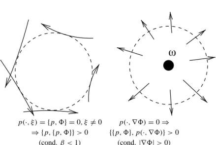
p(·, ξ )= {p, } =0, ξ =0 p(·,∇)=0⇒ ⇒ {p,{p, }}>0 {{p, },p(·,∇)}>0
(cond.β <1) (cond.|∇|>0)
Figure 1 – Graphical interpretation of pseudoconvexity for= |x−x0|2−βt2(waves) with increasing velocity from the outer to the inner levels of. p =ξ02− |ξ|2is the principal symbol ofP∗. Left: rays are bicharacteristics, right: arrows are∇.
0
=ct
Φ
Γ
0=
∂Ω
x
0
x
0
=ct
Φ
Γ
∇·n <0 outsideŴ0 ∇·n<0 outsideŴ0
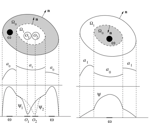
Ŵ0is the whole boundary Ŵ0is the exit/lateral part of the boundary Figure 2 – Graphical interpretation of the strong Lopatinskii condition for = |x−x0|2−βt2(waves) in the cases thatx0is inside and outside of the domain. The level sets of the weightare represented by the dotted lines.
wherenis the unit exterior normal to,pi are polynomial weights (see Table 2) andρ is the weight function given by (1). Notice thatρ →0 exponentially as
The internal observational or control regionωappearing at the right hand side of the global Carleman inequality is such that the pseudoconvexity of with respect toPq∗holdsoutsideω(for pseudoconvexity notion see [20], [43]). The boundary observational or control region Ŵ0 is such that a strong Lopatinskii condition holds outsideŴ0(see Table 1). If the condition of pseudoconvexity is satisfied in all×I then ωcan be empty. Also, if the strong Lopatinskii condition holds on all∂thenŴ0can be empty (see [43] for a much more general statement of global Carleman inequalities in this cases).
outsideω outsideŴ0 Condition |∇ψ (x)|>0 ∇ψ (x)·n<0
(necessary to pseudoconvexity) (strong Lopatinskii)
Table 1 – Pseudoconvexity and strong Lopatinskii conditions could not be satisfied in the internal and boundary observational/control regions.
Equation p1 p0 Heat sλ2 s3λ4 Wave sλ s3λ3 Schrödinger sλ s3λ4
Table 2 – Polynomial weights in global Carleman inequalities.
Some variants we consider in this review appear when considering operators withdiscontinuous coefficientsin the principal part. In this case, the functionψ has to be well adapted to this new situation and specific global Carleman estimates can be derived. In both cases, some spatial monotonicity of the coefficients is needed. As an application of these inequalities, we study one measurement inverse problems for the heat and wave equations using the general Bukhgeim-Klibanov approach [11]. The results explained here have been collected from the articles [13], [6], [7] and the preprint [2].
Other interesting variants we consider here arise in the case ofmobile domains
other hand due to the presence of the structure. The results we present in this review were adapted from the articles [9], [10].
The last variant is concerned with one measurement inverse problems from
local boundary observationsfor the wave equation. In this case, the function ψ is modified in order to obtain some strong Lopatinskii condition of the form (x−x0)·T n < 0, whereT is some linear transformation of the normal field. For further details we refer to the article [14] where the Carleman weights were introduced for two dimensional domains. Here we explain how to deal with the three dimensional case.
Although this is a reduced selection of variants, this collection of Carleman weights and applications illustrate the wealth of the extent of Carleman inequal-ities when they are applied to the study of some singular inverse and controlla-bility problems.
2 Inverse source problem for heat transmission problems
Given⊂Rnbe a bounded and regular subset and let1be a subdomain such that1 ⊂ and let us set0 = \1. LetS be the interface between 0 and1with unit normalnexterior to1. Let us denote byS+andS−the outer and inner sides of the interface S with respect ton and+ = S+ ×(0,T), − =S−×(0,T).
Let us consider the heat transmission problem
yt−div(a0(x)∇y)= f(x)g(x,t) in 0×(0,T)
yt−div(a1(x)∇y)= f(x)g(x,t) in 1×(0,T)
y|+ =y|−, a0 ∂y
∂n|+ =a1
∂y
∂n|−, y =0 on ∂×(0,T) (∗)
(7)
withai ≥c0>0 a.e. in. Let us introduce the space
V =y∈C2(i× [0,T]), i =0,1, ysatisfies(∗)
. (8)
some isotopy type condition is satisfied (see Figure 2 and the details in the article [13]). The inverse stability result is
Theorem 2.1 ([6], [7]). Let T0∈(0,T)andω0⊂0and let us assume that1
and0satisfy the isotopy type conditions of[13]. Assume that y solution of(7)
such that y,yt ∈V . Assume that a1|S−−a0|S+ ≥0and that g ∈C2(×[0,T]), |g(·,T0)| ≥ r0 > 0a.e. in. Then there exists a constant C =C(g, ω0,T0)
such that for all f ∈ L2()
fL2() ≤C y(·,T0)H2(0)+ y(·,T0)L2(1)+ yH1(0,T;L2(ω0)). (9) This result has as main ingredient a global Carleman estimate for the system (7) stated in [13]. This inequality was firstly used in order to prove the exact controllability to trajectories for a semilinear system similar to (7) that is con-trolled inω0×(0,T). In the general case when1is not simply connected, and in order to construct the weight functions, an isotopy type condition betweenS
and the boundary of two disjoint open subsetsOi,i =1,2 of1is used. Two weights similar to (3) are then constructed of the form
i(x,t)=
exp(λα)−exp(λψi(x))
T −t , i =1,2, (10)
whereψi ∈ V and∇ψ =0 only inOi (see Figure 1 left). Notice that you can
also consider the opposite case when 0 ⊂ and1 = \0, and always ω0⊂0. In this case, an isotopy type condition between∂andSis a sufficient condition. See Figure 1 right).
3 Controllability problems in mobile domain for fluid-structure interaction
Let⊂R2be a fixed bounded connected open subset with regular boundary. We denote respectively byS(t)andF(t)=\S(t)the domains occupied
by the structure (we consider here only one connected component of solid but the results shown here are still valid for a finite number of solids) and by the fluid respectively. Letn be the unit exterior normal to ∂S(t). The time evolution
O2
a
0
a
0 a1
ψ
2O
1
Ω1 Ω0
O1 O2
ψ
1ω
nω
ω
n 1 Ω0a
1a
0a
1ω
ψ
Ω nω
nFigure 3 – Construction of the global Carleman weight (bottom curves) for the heat equation with discontinuous coefficients such thata1(S−)−a0(S+) >0 (middle curves). In the case0⊂(left) two combined weights are used and in the case1⊂(right) one weight suffices. In both cases the observation zoneωis represented by a black dot.
the incompressible Navier-Stokes equations where the Cauchy tensorσ (u,p)= ν(∇u+ ∇ut)− pId with viscosityν > 0 will appear. The movement of the
rigid solid with massm >0 and moment of inertia J >0 is described by the velocity of its center of massa(t) ∈ R2 and by its angular velocityr(t)
∈ R. The system is
∂tu+(u· ∇)u−divσ (u,p)= f1ω, divu =0 in F(t) ma¨ =
∂S(t)
σ (u,p)ndσ, Jr˙ =
∂S(t)
(σ (u,p)n)·(x −a)⊥dσ,
u= ˙a+r(x−a)⊥on ∂S(t),u =0 on ∂,
u(0,·)=u0in F(0),a(0)=a0, a˙(0)=a1,r(0)=r0,
(e) (d)
(c)
(a) (b)
(e) (d)
(b) (c)
(a)
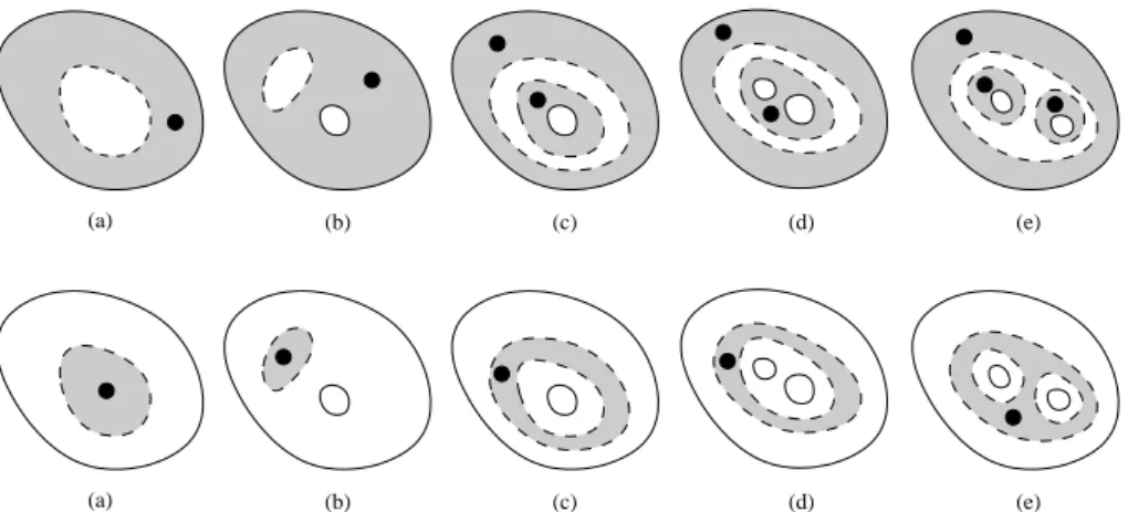
Figure 4 – In all the figures0is filled in gray and the observation regionωis represented by a black dot. The interfaceSbetween0and1is represented by a dashed line and the boundary∂by a solid line. In the lower line, all the examples except for (b) and (d) satisfy the isotopy type condition of [13] betweenSand∂. In the upper line, all the examples except for (e) satisfy the isotopy type condition betweenSand the boundaries of two disjoints subsets O1andO2of1. In all the exceptions, the Carleman weight can not be constructed with the method of [13].
Here the function f is thecontrolfunction which acts over a fixed small non-empty open subsetω(with characteristic function 1ω). See Figure 5.
n
(t)
F
Ω
S(t)(a,a,r)
Ω
O (u,p)
δ
δ ω
Ω
We have used the notation x⊥ = (x1,x2)⊥ = (−x2,x1). The total angleθ associated to the angular velocityr is defined byθ (t)=θ0+0tr(s)ds,where θ0 ∈ Rcomplements the initial data. The existence of solutions and regularity for this system has been recently studied in several papers (see [39], [41] and the references therein).
The controllability result is the following, saying that it is possible to drive the structure and the fluid at rest and the immersed solid up to its reference position in arbitrarily small time with a localized control f, provided the initial conditions are sufficiently small.
Theorem 3.1 ([9]). Suppose that: i) the initial body solid shape satisfies
S(0)⊂\ω, d(S(0), ∂(\ω)) >0,
∂S(0)
(y−a0)dσ =0; (12)
i i) the initial conditions u0 ∈ H3(F(0))2, a0 ∈ R2, a1 ∈ R2, θ0 ∈ Rand
r0 ∈Rsatisfy the compatibility conditions divu0=0 in F(0),
u0=a1+r0(x −a0)⊥ on ∂S(0) and u0=0 on ∂;
(13)
i i i) the acceleration u1 of the fluid and the accelerations a2 and r1 of the
structure at initial time (determined by the equations of the motion (11) and by the boundary conditions taken at initial time, well defined thanks to Helmholtz decomposition) satisfy
u1 =0 on ∂,
u1 =a2+r1(x−a0)⊥−r02(x−a0) − ∇u0 a1+r0(x −a0)⊥
on ∂S(0).
(14)
Under the above assumptions, for all T > 0 there exists ε > 0 and f ∈ L2((0,T)×ω)2such that if
u0H3(
F(0))2 + |a0| + |a1| + |θ0| + |r0| ≤ε
then
The last condition in (12) is a symmetry restriction over the shape of the solid needed in the proof of the Carleman inequality satisfied by the adjoint problem of the linearized system to get estimates on the structure motion from estimates on the fluid velocity on the interface.
The result only holds for small initial data because we want to keep the non-collision condition on the whole interval(0,T)
inf
t∈(0,T)d(S(t), ∂(\ω)) >0.
The first result of this kind using global Carleman estimates was obtained in [12] for a one-dimensional Burgers-particle system studied in [45]. Also, similar results to the one presented here has been simultaneously and independently obtained in the preprint [12] (see the preprint version of [10]).
The idea of the proof is the following and follows ideas for the controllability of the Navier-Stokes equations recently used in [15], [21] and the ideas of [12]. We first consider a linearized problem. Let(a˜,r˜)be given inH2(0,T)2×H1(0,T). We defineθ˜the angle associated to the rotation velocityr˜defined up to a constant. For anyt ∈(0,T), we define the structure domain
S(t)=
˜
a(t)+Rθ (˜t)−θ0(y−a0), y∈S(0)
.
We suppose thata˜(0) = a0, θ (0)˜ = θ0and inft∈(0,T)d(S(t), ∂(\ω)) > 0.
Thus, we can define the fluid domain F(t) = \S(t). We also consider
a given velocityu˜ satisfying regularity properties and compatibility conditions with(a˜,r˜). The linearized problem associated to (11) is the one where we have replaced in (11)S(t)byS(t),F(t)byF(t)and the nonlinear term(u·∇)u
in the first equation by(u˜ · ∇)u. We prove a null controllability result for the linearized problem with the help of a Carleman inequality shown on the adjoint system associated to a linearized system. Finally, Theorem 3.1 is proved by applying Kakutani’s fixed point theorem.
Let us first introduce the corresponding adjoint operatorPq∗on this case given
by the solution(v,q,b, γ )of the linear system
−∂tv−(u˜ · ∇)v−divσ (v,q)=0, divv =0 inF(t), mb¨(t)= −∂
S(t)σ (v,q)ndσ,
Jγ (˙ t)= −∂
S(t)(σ (v,q)n)·(x− ˜a(t)) ⊥dσ,
v= ˙b+γ (x− ˜a)⊥on∂S(t), v=0 on∂,
v(T,·)=vT
0 inF(T),b(T)=0, b˙(T)=b
T
1, γ (T)=γ
T
0 ,
(15)
with
divv0T =0 in F(T),
v0T =b1T +γ0T(x− ˜a(T))⊥ on ∂S(T) and
v0T =0 on ∂
(16)
andu˜ regular enough and conveniently chosen.
The following extremal weights appear when eliminating the explicit depen-dence on the pressureqof the Carleman inequality. For a given fieldv(x,t)we take the notation:
v(t)= sup
x∈F(t)
v(x,t), v(t)= inf
x∈F(t)
v(x,t). (17)
Theorem 3.2 ([9]). There existss,ˆ λˆ and C depending on,ωand T such that, for every regular solution(v,b, γ )of(15), for allλ >λˆ and s>s we have:ˆ
T
0
F(t)
ρ2
1
sϕ |v| 2
+ |∂tv|2
+sλ2ϕ|∇v|2+s3λ4ϕ3|v|2
d xdt
+sλ T
0
ρ2ϕb¨2+ | ˙γ|2
dt
T
0
∂S(t)
ρ2s3λ3ϕ3|v|2∇ψ·n+2sλϕ|∇vn|2dσdt
≤Cs19/2λ13 T
0
ω
(ρ/ρ)2ρ2ϕ10|v|2d xdt.
(18)
The Carleman inequality is expressed on themovingdomainsS(t)andF(t)
used here is of the form (compare with (3))
(x)= exp(λα0)−exp(α1λψ (x,t))
(T −t)4 (19)
whereα0, α1are suitable constants. The time dependent weight functionψ(x,t) is chosen as the standard weight for the heat equation but it follows the shape ofS(t). More precisely,ψ(x,t)is a regular function such that ∂ψ∂n <0 on,
|∇ψ| > 0 outsideωand it satisfies the time dependent conditions ∂ψ∂n > 0 on ∂S(t), ψ constant on ∂S(t). Notice that an interesting property is that the
spatial gradient ofψis related to 1/δ(t), whereδ(t) >0 is the distance between
S(t)and∂(\ω). This could be useful when doing explicit calculations of
constants in the Carleman inequality as the collision parameterδ(t) → 0+as
t →t0−for some collision timet0>0.
4 Inverse problem in wave equation with partial boundary data
The main idea is to modify the weight functiongiven in (4) in such a way that its gradient∇a rotation of the original field(x−x0)with a radially dependent magnitude. This concept come up from multipliers technique and controllability [19], [34].
Letbe a domain inRn,n
=2,3. In order to solve the Dirichlet to Neumann one measurement inverse problem, it suffices to measure on arotated exit part
of the boundaryŴr. Ifn =2, this region depends on a pointx0 ∈ Rn and on a rotationTθ in an angleθ ∈ (−π/2, π/2). Ifn =3, it depends also on a unit directionα∈R3and the rotationTθ is considered on the orthogonal plane toα denoted here byα⊥. We will use the notationv⊥=v−(v·α)αfor the projection of the fieldvonα⊥. More precisely
dot product between the vectorx −x0and the projectionn⊥ rotated inπ/2 is positive (see Figure 6). There are of course an infinite number of intermediate cases depending on the localization of x0, the direction ofα and the angle θ. The caseθ =0 corresponds to the standard exit condition previously used for the same inverse problem [24]. Remark also that the rotated exit condition is a particular case of the geometrical optics BLR condition [1], [33].
The main stability result is the following (we present here the casex0 ∈ , the other case in which two arbitrarily near interior points are used can be found in [14]).
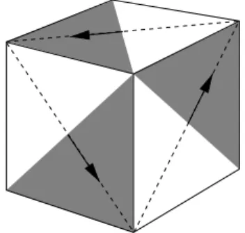
Figure 6 – Rotated exit boundary region in a cube(−a,a)3with respect to the origin
x0=0 and a diagonal axisαparallel to(1,1,1)with orthogonal planeα⊥(dotted lines). The exit region (shaded) are the boundary points whose position vectors have a positive dot product with theπ/2 rotation of the projection of the normaln⊥onα⊥(arrows). By taking a suitable time-dependent Neumann measure on a little bit more than this region, the inverse problem of recovering a time-independent potential in the wave equation is locally stable (not really in a cube but in a regularizedC2cube).
Theorem 4.1 ([14]). Let Pq∗ = ∂t t −+q and let u(q)and u(q)be the re-spective solutions of Pq∗u =0with Dirichlet boundary conditions associated to q,q ∈ L∞()and with Neumann measurementsξandξonŴr×(0,T) respec-tively. There exists a time T >0such that if T >T , if u(q)∈ H1(0,T;L∞())
and if|u(0)| ≥ α0 >0a.e. in, then there exists a positive constant CM de-pending on M = qL∞()such that
||q−q||L2() ≤CM
ξ −ξH1(0,T;L2(Ŵ
Ifθ → ±π2 then T → +∞and it behaves asymptotically as
T ≈ √R0
β exp
2 cosθθ0
, (23)
where R0=supx∈|x−x0|andθ0=supx∈arg(x−x0)⊥−infx∈arg(x−x0)⊥,
i.e., the angle of view ofwith respect to the axis of directionαpassing by x0. The proof of this Theorem is based on a global Carleman estimate using the variant of the Carleman weight for the wave equation (compare with (4))
(x,t)= −λexp cosθ|x −x0|2 exp 2 tanθarg(x−x0)⊥
−βt2 (24) for some suitable constantβ ∈ (0,1). This weight was constructed in order to make appear in the gradient∇the matrix
cosθ 0 0
0 cosθ sinθ 0 −sinθ cosθ
(25)
written in a basis attached toα, α⊥. The product of this matrix and a vector field v is exactly cosθ (v−v⊥)+Tθv⊥, expression which appears in the definition (21) ofŴr.
The main steps in the deduction of such inequality are taken from [35, 23] following a well known technique due to Bukhgeim and Klibanov [11], [29]. Roughly speaking, the technique in this case consists in reducing the problem to a source inverse problem for the perturbed equation aroundu(q)and then take its time derivative in order to obtain a quasi-observability inequality after use of the Carleman inequality. Quasi, since the initial condition is bounded not only by the observation but also by the unknown source term, but a sufficiently large time and the properties of the Carleman weight allow to get rid of this source term.
optic condition are not necessary to solve the one measurement inverse prob-lem (see [27]). Other completely different probprob-lem is the case when you have Dirichlet to Newmann map measurements. In this case, a suitable arbitrarily small boundary of measurements is enough to solve the inverse problem both for Schödinger and wave equations (see [28]). But recently, it has been shown that you can solve the one measurement problem for the wave equation with an arbitrarily boundary measurement region (in the case of Neumann bound-ary conditions and Dirichlet measurements), but the corresponding inequality analogous to (22) is logarithmic [5].
5 Inverse coefficient problem for wave transmission problems
Notice that recently, Global Carleman estimates and application to one mea-surement inverse problems for the wave equation were obtained in the case of variable but still regular coefficients [4], [26]. The inverse problem of retrieving coefficients from a wave equation with discontinuous coefficients from bound-ary measurements arise naturally in geophysics and more precisely, in seismic prospection of earth inner layers [44].
Letand1⊂be two open subsets ofR2with smooth boundariesŴand Ŵ1respectively and let2=\1. To fix ideas we assume that1is simply connected. We set:
¯
a(x)=
a1 x ∈1
a2 x ∈2
(26) withaj >0 for j =1,2, for eachq ∈ L∞(), we consideru(q)as the solution
of the following wave transmission equation
ut t −div(a¯(x)∇u)+q(x)u=0 in Q=×(0,T)
u =g on =Ŵ×(0,T)
u(0)=u0 in
ut(0)=u1 in.
(27)
The following inverse stability result holds (see the preprint [2]):
Theorem 5.1 ([2]). Assume1isstrictly convexand a1>a2>0. LetUbe a
and u(q)∈ H1(0,T;L∞()), then there exists C =C(,T,qL∞(),U) > 0such that:
q−qL2()≤C
∂u(q) ∂n −
∂u(q) ∂n
H1(0,T;L2(Ŵ))
for all u0∈ H01()and q∈U.
This Theorem is proved by combining the Carleman inequality for the wave equation with discontinuous coefficients proved in [2] and the method of Bukh-geim-Klibanov explained in section 4. To this end, system (27) is viewed as two wave equations with constant coefficients coupled with transmission conditions (see [31]). Then, a global Carleman inequality is found out for this transmission problem by working with variants of Carleman weights of the form (compare with (4))
(x,t)= −exp(λϕ(x)), (28)
ϕ(x)=
η(x) a2
r(x)2|x −x0|
2−βt2+M
1 in 1×(−T,T)
a1
r(x)2|x−x0| 2
−βt2+M2 in 2×(−T,T)
(29)
whereM1andM2are constants such thatM1−M2=a1−a2,r(x)= |x0−y(x)|,
y(x)=Ŵ1∩ [x0,x]andηis some cut-off function with support in1centered atx0. We also combine the Carleman inequalities obtained from two different interior points as we did in section 2, see also Figure 1, left. The convexity hypothesis on1comes from the fact that the positiveness of the Hessian of the weightis related with the curvature ofŴ1with respect tox0.
REFERENCES
[1] C. Bardos, G. Lebeau and J. Rauch,Sharp sufficient conditions for the observation, control and stabilization of waves from the boundary. SIAM J. Contr. Optim.,30(1992), 1024–1465. [2] L. Baudouin, A. Mercado and A. Osses,Global Carleman estimates in a transmission problem
for the wave equation. Application to a one-measurement inverse problem, Inverse Problems,
23(2007), 1–22.
[3] L. Bauduoin and J.-P. Puel,Uniqueness and stability in an inverse problem for the Schödinger equation. Inverse Problems,18(6) (2002), 1537–1554.
[4] M. Bellassoued,Uniqueness and stability in determining the speed of propagation of second-order hyperbolic equation with variable coefficients. Appl. Anal.,83(10) (2004), 983–1014. [5] M. Bellassoued and M. Yamamoto,Logarithmic stability in determination of a coefficient in an acoustic equation by arbitrary boundary observation. J. Math. Pures Appl.,85(2006), 193–224.
[6] M. Bellassoued and M. Yamamoto,Inverse source problem for a transmission problem for a parabolic equation. J. Inv. Ill-Posed Problems,14(1) (2006), 47–56.
[7] A. Benabdallah, P. Gaitan and J. Le Rousseau,Stability of discontinuous diffusion coefficients and initial conditions in an inverse problem for the heat equation. Preprint LATP – Labo-ratoire d’Analyse, Topologie, Probabilités, CNRS: UMR 6632, Université Aix-Marseille I, France, May 2006.
[8] G. Beylkin,The inversion problem and applications of the generalized Radon transform. Comm. Pure Appl. Math.,37(5) (1984), 579–599.
[9] M. Boulakia and A. Osses,Two-dimensional local null controllability of a rigid structure in a Navier-Stokes fluid. C.R. Math. Acad. Sci. Paris., Ser. I,343(2) (2006) 105–109. [10] M. Boulakia and A. Osses,Two-dimensional local null controllability of a rigid structure in
a Navier-Stokes fluid. Preprint 139, U. de Versailles Saint-Quentin, France, October 2005. To appear in ESAIM-COCV.
[11] A. L. Bukhgeim and M. V. Klibanov,Global uniqueness of a class of inverse problems. Dokl. Akad. Nauk SSSR,260(2) (1981), 269-272, English translation: Soviet Math. Dokl,
24(2) (1982), 244–247.
[12] A. Doubova and E. Fernandez-Cara,Local and global controllability results for simplified one-dimensional models of fluid-solid interaction, to appear in Math. Models Methods Appl. Sci.
[13] A. Doubova, A. Osses and J.-P. Puel,Exact controllability to trajectories for semilinear heat equations with discontinuous diffusion coefficients. A tribute to J. L. Lions. ESAIM Control Optim. Calc. Var.,8(2002), 621–661.
[15] E. Fernandez-Cara, S. Guerrero, O. Yu. Imanuvilov and J.-P. Puel,Local exact controllability of the Navier-Stokes system. J. Math. Pures Appl.,83(12) (2004), 1501–1542.
[16] A. Fursikov and O. Yu. Imanuvilov,Controllability of Evolution Equations. Lecture Notes,
34, Seoul National University, Korea, 1996.
[17] S. Hansen, Solution of a hyperbolic inverse problem by linearization. Comm. Partial Differential Equations,16(2-3) (1991), 291–309.
[18] A. Haraux,Séries lacunaires et contrôle semi-interne des vibrations d’une plaque rectan-gulaire. J. Math. pures et appl.,68(4) (1989), 457–465.
[19] L. Ho,Observabilité frontière de l’équation des ondes. (Boundary observability of the wave equation). C.R. Acad. Sci., Paris, Ser. I,302(1986), 443–446.
[20] L. Hörmander,The analysis of linear partial differential operators II. Springer-Verlag, Berlin, 1983.
[21] O. Yu. Imanuvilov,Remarks on exact controllability for the Navier-Stokes equations. ESAIM Control Optim. Calc. Var.,6(2001), 39–72.
[22] O. Yu. Imanuvilov and J.-P. Puel,Global Carleman estimates for weak solutions of elliptic nonhomogeneous Dirichlet problems. Internat. Math. Res. Notices,16(2003), 883–913. [23] O. Yu. Imanuvilov,On Carleman estimates for hyperbolic equations. Asymptot. Anal.,
32(3-4) (2002), 185–220.
[24] O. Yu. Imanuvilov and M. Yamamoto, Global uniqueness and stability in determining coefficients of wave equations.Commun. Partial Diff. Eqns,26(7-8) (2001), 1409–1425. [25] O. Yu. Imanuvilov and M. Yamamoto,Global lipschitz stability in an inverse hyperbolic
problem by interior observations. Inverse Problems,17(4) (2001), 717–728.
[26] O. Yu. Imanuvilov and M. Yamamoto.Determination of a coefficient in an acoustic equation with a single measurement. Inverse Problems,19(1) (2003), 157–171.
[27] S. Jaffard,Contrôle interne exact des vibrations d’une plaque rectangulaire, Portugal. Math.,
47(1990), 423–429.
[28] C. Kenig, J. Sjöstrand and G. Uhlmann,The Calderón problem with partial data, to appear. [29] M. V. Klibanov and J. Malinsky,Newton-Kantorovich method for three-dimensional poten-tial inverse scattering problem and stability of the hyperbolic Cauchy problem with time-dependent data. Inverse Problems,7(1991), 577–595.
[30] V. Komornik,Exact controllability and stabilization. The multiplier method, Research in Applied Mathematics 36, Paris, Masson, 1994.
[31] J.-L. Lions,Contrôlabilité exacte, perturbation et stabilisation de Systèmes Distribués, 1, Masson, Paris, 1988.
[33] L. Miller,Escape function conditions for the observation, control, and stabilization of the wave equation. SIAM J. Control Optim.,41(5) (2003), 1554–1566.
[34] A. Osses,A rotated multiplier applied to the controllability of waves, elasticity, and tangential Stokes control. SIAM J. Control and Optim.,40(3) (2001), 777–800.
[35] J.-P. Puel,Application of Carleman Inequalities to Controllability and Inverse problems, Textos de Metodos Matematicos de l’Instituto de Matematica de l’UFRJ, to appear. [36] J.-P. Puel and M. Yamamoto, Generic well posedness in a multidimensional hyperbolic
inverse problem, J. of Inverse and ill-posed problems,1(1997), 53–83.
[37] Rakesh,A linearised inverse problem for the wave equation. Comm. Partial Differential Equations,13(5) (1988), 573–601.
[38] Rakesh,An inverse impedance transmission problem for the wave equation. Comm. Partial Differential Equations18(3-4) (1993), 583–600.
[39] J. San Martín, V. Starovoitov and M. Tucsnak,Global weak solutions for the two dimensional motion of several rigid bodies in an incompressible viscous fluid. Arch. Rational Mech. Anal.,161(2) (2002), 113–147.
[40] W.W. Symes,A differential semblance algorithm for the inverse problem of reflection seis-mology. Comput. Math. Appl.,22(4-5) (1991), 147–178.
[41] T. Takahashi,Analysis of strong solutions for the equations modeling the motion of a rigid-fluid system in a bounded domain. Adv. Differential Equations,8(12) (2003), 1499–1532. [42] T. Takahashi and O. Yu Imanuvilov,Exact controllability of a fluid-rigid body system, Preprint
IECN, U. Nancy, France, november 2005.
[43] D. Tataru,Carleman estimates and unique continuation for solutions to boundary value problems. J. Math. Pures Appl., (9)75(4) (1996), 367–408.
[44] M. de Hoop,Microlocal analysis of seismic in inverse scattering. Inside out: in inverse problems and applications, 219–296. Math. Sci. Res. Inst. Publ.,47(2003), Cambridge Univ. Press, Cambridge.
[45] J.L. Vázquez and E. Zuazua, Lack of collision in a simplified 1-dimensional model for fluid-solid interaction, M3AS,16(5) (2006), 637–678.
[46] M. Yamamoto,Uniqueness and stability in multidimensional hyperbolic inverse problems. J. Math. Pures Appl.,78(1999), 65–98.