Using normal mode channel structure for narrow band underwater communications in shallow water

Using Normal Mode Channel Structure for Narrow Band Underwater Communications in Shallow water.

A. G. Silva , S. M. Jesus

Universidade do Algarve, Campus de Cambelas, 8000 Faro, Portugal.

Multipath and high temporal and spatial variability of the propagation environment causes severe signal degradation in shallow water acoustic digital communications. Among the many solutions that have been proposed most known is adaptive equalisation where cyclic training signals are used to adapt the equaliser to the variability of the acoustic channel. When the channel is rapidly changing, equaliser coefficients are frequently adapting and effective transmitting rate rapidly decreases. Another approach consists in using a priori information obtained from acoustic propagation models. These models can give a deterministic estimate of the true channel impulse response that can be used to detect the transmitted signals. In practice, the use of deterministic acoustic models is mainly dependent of the accuracy of the input environmental parameters. As a first step, this paper presents an exhaustive study of the signal detection sensitivity to model parameters mismatch. The scenario used is composed of a 100m depth water column with range dependent characteristics. The water column is located over a 10m thick sediment layer with variable properties. Source-receiver communication is made over a variable distance between 500 and 600m with the source near the bottom and the receiver near the surface. The communication signals are narrow band (1.5KHz) pulse amplitude modulated with a carrier frequency of 15KHz, and the detector is based on the Maximum-Likelihood Sequence Detector (MLSD).

I. INTRODUCTION

Detection of a digital signal sent by an acoustic source in a shallow-water environment is a difficult, yet interesting problem that has received a great deal of attention in the last few years [1]. Due to multipath and high temporal and spatial variability, the ocean environment causes severe degradation in the performance of communication systems. Additive noise, originated from Human and natural multiple sources, causes a relatively low Signal to Noise Ratio (SNR), that becomes of great importance when the source is located and has a limited power available. Among the many solutions that have been proposed to overcome these problems, adaptive equalisation presents the most effective results [2] for real time applications. In adaptive equalisation, cyclic training signals are used to adapt the equaliser to the variability of the acoustic channel. When the channel is rapidly changing, equaliser coefficients are frequently adapting and effective transmitting rate rapidly decreases. Array signal spatial diversity

processing, aiding equalisers, also presents good results [3]. Non-coherent modulation is still used on the implementation of robust systems but they have a poor spectral efficiency and a low transmission rate [4].

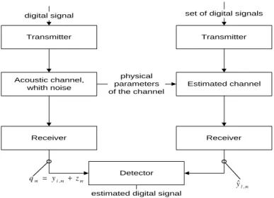
Another approach consists in using a priori information obtained from physical propagation models in order to determine how the transmitted signal is modified during its travel between the source and the receiver(s). Figure 1 shows a flow diagram of this approach: in the left side the digital signal travels through the true acoustic channel, and in the right side the set of possible digital signals travel through an estimated channel computed using the physical parameters of the true channel. In the detector both the receiver and the predicted signals meet to estimate emitted the digital.

It is commonly accepted that the wave propagation and the boundary interaction dominating shallow-water propagation can be well described by a normal-mode model

Acoustic channel, whith noise

Detector

estimated digital signal physical parameters of the channel Estimated channel Transmitter digital signal Transmitter set of digital signals

Receiver Receiver

qm = yi m, +zm _$

,

yl m

Figure 1 - Technical solution using a priori information obtained from acoustic propagation models. The idea pursued in this paper, is to

measure the degree of similarity between the estimated and the true channel impulse response and in that sense this technique can be referred as a model-based detection and has a strong analogy to matched-field processing being used in source localisation [5]. The detector is implemented using a Maximum Likelihood Sequence Detector since it is simple and optimal when the noise is white and gaussian. In practice, the use of deterministic acoustic models is mainly dependent on the accuracy of the input environment parameters. As a first step, this paper presents an exhaustive study of the signal detection sensitivity to model parameters mismatch. Particular emphasis is made on the source/receiver relative location, bottom characteristics, sound speed profile in the water column and channel geometry.

II. THEORY

A. Normal-mode modelling

The shallow-water ocean environment is modelled as a stratified wave-guide with an arbitrary sound-speed profile in the vertical. Long and medium range sound transmission in such environment can be described by the discrete normal-mode model [6]. The solution of the wave equation for a narrowband point source exciting an horizontal wave-guide is commonly expressed as a linear combination of wave-guide normal-mode depth functions.

For a monochromatic source the pressure at the receiver is given by the sum of the natural modes of vibration, and is approximately expressed by

( )

( )

( )

p r z e z r Z z Z z e k j s m s m jk r m m M m ( , )≈ − =

∑

π ρ π 4 1 8 . (1)

Where p r z

( )

, is the acoustic pressure as a function of depth z , and range r and ρ z is the

( )

density. The modal equation has a infinite number of solutions (modes), but only M of those, represent propagating modes. Those modes are characterised by a mode shape function Z_m

( )

z , and a horizontal propagation constant km

(horizontal wave number). One can also show that all the horizontal wave-numbers, are distinct and

( ) ( )

ω ω ω cb k k c z c z M w s ≤ < < ≤       ... ₁ max , , (2)

where cb, cw and cs are the sound speed in the

bottom, water and sediment respectively.For a narrowband point source one can compute the frequency response and then by Fourier synthesis the channel impulse response.

B. The Detector

From figure 1, a sampling version of the base-band equivalent signal after the receiver is

q_m = y_{i m,} +z_m, (3)

where y_{i m,} is one of L possible signals and represents the useful part of qm, and zm is a

zero-mean gaussian noise component. Considering that y_{i m,} = ∗h_m a_{i m,} (4)

where h_m is the impulse response of the channel, and a_{i m,} is one of the L possible digital signals, and that

$_, $ _,

y_{l m} = ∗h_m a_{l m}, for 1≤ ≤l L (5)

represents all the useful signals expected at the receiver. The detector can be implemented using a variant of the Maximum Likelihood Sequence Detector [7], shown in figure 2.

{ } Re + qm −1 2El Rl

{ }

max m $, * yl−m rl m, rl

Figure 2 - Variant of the Maximum Likelihood Sequence Detector.

This detector will compute L times

(

)

r_{l m} C_{h h} C_{a a} h _m a_{l m} z_m

i l

, = , $* , + $− ∗ ,− ∗

• ₍₆₎

where C represents the correlation function. According to figure 2 the detector will chose the sample of r_{l m,} that has maximum module, take the real part and subtract one half of the energy of the signal l . The decision will be made on the maximum R_l at the output. This detector will present the best results when the impulse response of the channel is known ( $h_m ≡h_m) and in presence of white gaussian noise.

III. TESTS AND RESULTS

The test case chosen in this paper is composed of a typical shallow water scenario of 100m depth water column with range dependent characteristics. The water column is located over a 10m thick sediment layer with variable properties. Source-receiver communication is made over a variable distance of 510m with the source near the bottom and the receiver near the surface.

The propagation model C-SNAP [8] was used to compute both the “true” acoustic channel and the estimate channel as sketched in figure 1. The mismatch between the two modelled channels is made by varying the physical parameters (one at a time). The communication signals are narrowband (1.5KHz) pulse amplitude modulated with a carrier frequency of 15KHz and a transmission rate of 750bits/seg. The mismatch environment parameters presented are the

source/receiver distance, the sound speed profile, the sediment characteristics and the bottom slope. The figure of merit will be the probability of error ( Pe ) versus the varying parameters and the signal to noise ratio (SNR).

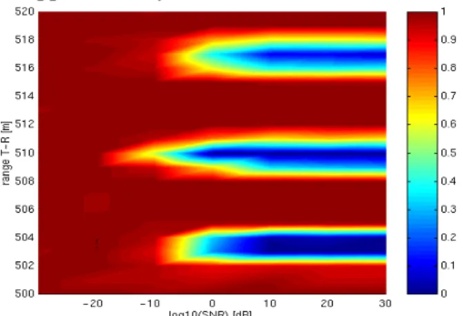
A. Source/receiver distance mismatch

For this parameter one considers that the source-receiver distance is varying between 500 and 520m. The results for this test are in figure 3. It can be seen that at 510m, where the channel impulse response matches the estimated one, the result is optimal with Pe≈0 for SNR>0dB; around the value of 510m the main valley is approximately 2m wide, for Pe attaining values of approximately 0.6.

Figure 3 – Probability of error versus receiver location mismatch (m) and SNR (dB).

One can also see that convergence zones are obtained within 7m from the main detection peak. These convergence zones are analogous to the mode/ray convergence zones found in monochromatic sound propagation [9]. In our case they can be found at the distance that simultaneously satisfies the modal interference distance for all the frequencies of the band. This “band interference distance” depends on the horizontal wave numbers and it will be seen later that the environment characteristics that change km will change the location of the convergence

zones.

B. Sound speed profile mismatch

In figure 4 one can see a typical summer sound speed profile. The mismatch will be obtained by moving point (4) between 1509.2 and 1510.8m/s.

1510 1503 1500 c(m/s) z(m) (4) (3) (5) (6) v 40 15 100 0

Figure 4 - Sound speed mismatch .

Figure 5 - Probability of error versus sound speed mismatch (m/s) and SNR (dB).

The result is shown in figure 5, where the no mismatch case is for a sound speed of 1510m/s. One can see that for a difference of 0.2m/s between the sound speed and its estimate, the Pe increases to 0.3 for SNR>10dB, and one can also see the appearance of a convergence zone due to the influence of the sound speed in the horizontal wave number.

C. Sediment characteristics mismatch

In C-SNAP code the sediment is modelled as a fluid and mainly characterised by the compressional attenuationα_p, density ρ_b and sound speed c_p. In table 1 one can see those characteristics for different kinds of sediments, from a soft one (silt) to a hard one (moraine).

Sediment α p ρb cp Silt 1.0 1.7 1575/1580 0.9 1.8 1612/1617 Sand 0.8 1.9 1650/1655 0.7 1.95 1725/1730 Gravel 0.6 2.0 1800/1805 0.5 2.05 1875/1880 Moraine 0.4 2.1 1950/1955

Table 1 - Sediment characteristic parameters. In figure 6, the no mismatch case corresponds to an attenuation of 0.7 and one can see that a variation of several orders of magnitude in the sediment softness results in only a few percent of performance degradation.

Figure 6 - Probability of error versus sediment mismatch and SNR (dB).

D. Bottom slope mismatch

The results in figure 7 show that the detector is highly sensitive to bottom slope. It also shows the appearance of convergence zones on both sides of the main valley. These convergence zones are not symmetric due to a highly concentration of energy for positive bottom slopes.

Figure 7 - Probability of error versus bottom slope mismatch and SNR (dB)

IV. CONCLUSIONS AND

PERSPECTIVES

When there is no parameters estimation error the channel impulse response is known and in the detector Pe≈0 for SNR>0dB as it was expected theoretically for a maximum likelihood detector. When only an estimate of the channel parameters is available, the detector performance decreases as the parameters estimation error increases. Considering the shape of the detector performance around the true value it can be seen that for SNR<10dB the Pe is dominated by noise while for SNR>10dB the detector performance is dominated by the quality of the match between the measured and estimated channel response. It was also shown that for receiver location mismatch, convergence zones appeared with a performance closer to the optimum. A mismatch in environmental parameters may change the location of the convergence zones. It was also found that a variation of several order of magnitude on sediment softness results in only a few percent of performance degradation.

In general the detector is very sensitive to model parameters mismatch, but the appearance of convergence zones can be an advantage that together with array processing may be explored in future work.

REFERENCES

[1] M. Stojanovic, “Recent advances in high-speed underwater acoustic communications”, IEEE Journal of Oceanic Eng., Vol. 21, No. 2, 1996.

[2] M. Stojanovic, J. A. Catipovic and J. G. Proakis, “Phase coherent digital communications for underwater acoustic channels”, IEEE Journal Oceanic Eng., vol. 19, 1994. [3] D. Thompson, J. Neasham, B. S. Sharif, O.R. Hilton, and A. E. Adams, “Performance of coherent PSK receivers using adaptive combining and beamforming for long range acoustic telemetry”, 3th European Conference on Underwater Acoustics, Greece, 1996.

[4] J. Capitovic, M. Deffenbaugh, L. Freitag and D. Frye, “An acoustic telemetry system for deep ocean mooring data acquisition and control”, in Proc. OCEANS’89, Seattle, WA, 1989.

[5] S. M. Jesus, “Normal-mode matching localization in shallow water: Environment and system effects”, J. Acoust. Soc. Am. 90 (4), 1991.

[6] Ivan Tolstoy and C. S. Clay, “Ocean Acoustics”, American Institute of Physics, 1966,1987.

[7] E. A. Lee, D. Messerschmitt, “Digital Communication”, Kluwer Academic Publishers, second edition, 1994.

[8] C. M. Ferla, M. B. Porter and J. B. Jensen, “Coupled SACALNTCEN normal mode propagation loss model”, Saclant Undersea Research Centre, 1993.

[9] Finn B. Jensen, William A. Kuperman, Michael B. Porter and Henrik Schmidt, “Computational Ocean Acoustics”, American Institute of Physics, 1993.