Cumulus boundary layers in the atmosphere : high resolution models and satellite observations

(1)

Universidade de Lisboa

Faculdade de Ciências

Departamento de Engenharia Geográfica, Geofísica e Energia

Cumulus Boundary Layers in the Atmosphere: High

Resolution Models and Satellite Observations

João Paulo Afonso Martins

Doutoramento em Ciências Geofísicas e da Geoinformação

(Meteorologia)

(2)

Universidade de Lisboa

Faculdade de Ciências

Departamento de Engenharia Geográfica, Geofísica e Energia

Cumulus Boundary Layers in the Atmosphere: High

Resolution Models and Satellite Observations

João Paulo Afonso Martins

Doutoramento em Ciências Geofísicas e da Geoinformação

(Meteorologia)

Tese Orientada por:

Prof. Pedro M. A. Miranda

Dr. João Teixeira

(3)

i

Acknowlegements

I would like to thank my two advisors, Prof. Pedro Miranda and Dr. João Teixeira not only for their scientific guidance, friendship and motivation, but also for the opportunity of working in three fantastic teams, one at Lisbon at Instituto Dom Luiz, and the other two in Los Angeles, California. In the first two years of this project I had the opportunity to meet amazing people from the Department of Atmospheric and Oceanic Sciences of the University of California at Los Angeles. In the last two years I have spent 6 months at NASA‟s Jet Propulsion Laboratory in Pasadena where I have met some of the smartest, funniest and competent people I have ever worked with. I will definitely never forget the time I have spent working there. I would like to thank in particular to those that I have met on those places who gave their support to make this thesis a reality. From my time at UCLA, Louise, Sergio, Katy, Greg, Celestino and Sambingo; from my time at JPL: Johannes, Jenny, Brian, Kay, Mathias, Qing, George, Daniel, Eric, Evan, Bill and Van. The discussions we had definitely improved the content of this work.

Of course I cannot forget home. My institute gave me all the tools, the knowledge and the support I needed. I cannot stress enough how grateful I am to Pedro Soares for dealing with my bad humor, successes, frustrations, distractions, (bad) jokes and deadlines… Thank you Pedro, I really enjoyed working with you for the past 4 years and I hope we can keep doing it for a long time. This acknowledgement has to be evidently extended to Ricardo and Emanuel, as they had to deal with all this on a daily basis as well for the whole course of this project. A big thanks to my other colleagues and friends, that in one way or the other helped me reaching my goals. I would also like to thank to the people outside the academic world, my family and friends for their constant support, friendship and love.

I acknowledge the funding I received from the Portuguese Science Foundation (FCT), under the doctoral grant SFRH/BD/37800/2007. I also acknowledge the funding I received from Fundação Calouste Gulbenkian by the “Programa Gulbenkian de Estímulo à Investigação” which helped in some of the expenses and also for funding from the FCT projects REWRITE (PTDC/CLI/73814/2006). IDL is funded by the FCT under the project PEST-OE/CTE/LA0019/2011/2012.

(6)

iv

Abstract

This project intends to explore some of the challenges on the representation of the Planetary Boundary Layer (PBL) using both high resolution models and state of the art observations. Some of the issues related the different types of boundary layers are highlighted in the context of a model intercomparison at a transect in the northeast Pacific that served as a benchmark for studying cloud regimes and transitions between them. Several model biases were detected and even reanalysis products do not show reasonable comparisons against observations in terms of low-cloud related variables. The transition from shallow to deep convection over land is a key process in the diurnal cycle of convection over land. High resolution simulations were analyzed the ability of the model to reproduce observed precipitation characteristics and its sensitivity to horizontal resolution and to the evaporation of precipitation. The latter physical process influences the development of new convection by increasing the thermodynamic heterogeneities at the PBL through the formation of cold pools which result from convective downdrafts. At the later stages of the transition these features dominate the PBL behavior, as the turbulent length scales increase up to several times the size of the PBL height. Results are however quite sensitive to model resolution. At the observational perspective, the Atmospheric Infrared Sounder was used to characterize the PBL properties in a variety of situations. An algorithm for PBL height determination was developed and validated against radiosondes launched at the Rain in Cumulus over the Ocean campaign. The encouraging results of the validation led to the calculation of a PBL height climatology over the tropical, subtropical and midlatitude oceans. Results were then compared to similar estimates from collocated profiles from ERA-Interim, revealing similar geographical distribution and seasonal variations. Diurnal variability is much different between both datasets which warrants further investigations.

(7)

v

Resumo

A camada limite planetária (CLP) apresenta desafios tanto em termos observacionais como em termos da sua modelação numérica. O seu papel no sistema climático traduz-se na mediação das interacções entre a superfície e a troposfera livre, através de fluxos turbulentos de calor, humidade , momento e outros constituintes químicos e aerossóis. A estrutura da CLP encontra-se profundamente relacionada com as condições climatéricas de uma dada região, em particular com tipo de nuvens predominantes. A intercomparação de modelos realizada sobre uma secção no Pacífico nordeste pretendeu avaliar a capacidade dos modelos de representar os diversos processos associados aos diversos regimes de nuvens presentes na região. A secção mostrou-se indicada para este exercício, pois além de amostrar as características principais das células de Walker e Hadley, é também representativa das transições que ocorrem entre nuvens estratiformes que ocorrem ao largo da costa da California, nuvens tipo cumulus pouco profundos na região dos Alíseos e nuvens tipo cumulonimbos que ocorrem preferencialmente na Zona Intertropical de Convergência (ITCZ). Os resultados da comparação evidenciaram as enormes discrepâncias que existem entre modelos em termos da representação dos processos associados às nuvens. Além dos modelos, a própria reanálise ERA-40 mostrou diferenças significativas quando comparada com observações de detecção remota dedicadas a esses processos.

A transição de entre convecção pouco profunda para convecção profunda é o processo que domina a fase matinal do ciclo diurno da convecção sobre terra nos trópicos, e a sua representação na maioria dos modelos de larga escala apresenta graves deficiências, com o pico da precipitação a ocorrer no período na manhã, enquanto as observações mostram que o mesmo ocorre a meio da tarde. Os modelos tendem a usar um fecho para a parameterização da convecção baseado no conceito de energia potencial disponível para a convecção (CAPE), que activa a convecção profunda demasiado cedo, sendo que as simulações de alta resolução têm mostrado que o processo é bastante mais gradual: inicia-se com a formação de uma camada limite bem misturada, seguida da formação de cumulus pouco profundos que humidificam as camadas inferiores da troposfera, para então se dar a transição para convecção profunda. Neste projecto realizaram-se simulações de alta resolução deste processo usando o modelo MesoNH, por forma a estudar a capacidade do modelo de reproduzir as características da precipitação e a sensibilidade dos resultados à resolução do modelo e à evaporação da precipitação. Este

(8)

vi

último processo físico desempenha um papel fundamental no estabelecimento da fase madura do regime de convecção profunda. Isto porque ao evaporar, a precipitação arrefece o ar, causando fortes correntes descendentes que ao atingir a superfície se espraiam sob a forma de correntes gravíticas. Nos limites destas correntes, fortes gradientes termodinâmicos forçam o ar da CLP a subir, originando novas térmicas que eventualmente formam novas células convectivas. Nas fases finais da transição, estas perturbações dominam o comportamento da CLP, tal como indicam os diagnósticos espectrais das escalas de comprimento dominantes. Esta análise mostra que o tamanho dos turbilhões na CLP varia desde a dimensão típica da altura da CLP na fase de convecção pouco profunda até dimensões que superam várias vezes essa escala típica na fase de convecção profunda. Esse comportamento é totalmente distinto na simulação sem evaporação de precipitação, com os turbilhões a manterem dimensões associadas à altura da CLP durante todo o processo. Os resultados revelam contudo uma grande sensibilidade à resolução do modelo, com evoluções bastante distintas no alcance vertical da convecção nas simulações com diferentes resoluções. As diferenças são atribuidas à diferente representação dos processos turbulentos por parte do modelo de turbulência de subescala, mas os resultados são ainda inconclusivos.

A observação da CLP por métodos de detecção remota apresenta também desafios próprios. Neste projecto, a base de dados do Atmospheric Infrared Sounder (AIRS) V5 L2 Support Product foi usada para estimar parâmetros da camada limite. Este produto apresenta um espaçamento de grelha vertical superior ao dos produtos AIRS convencionais, o que o torna mais indicado para estudar a CLP. Um algoritmo para determinação da altura da CLP foi desenvolvido e validado contra dados das sondagens lançadas no contexto da campanha Rain in Cumulus over the Ocean, ocorrida nas Caraíbas no Inverno de 2004-2005. Essa área é dominada nessa altura do ano por convecção pouco profunda embebida nos ventos alíseos, o que a torna ideal para a validação dos perfis obtidos com o AIRS, dado que o sensor utiliza radiâncias da banda do infravermelho, fortemente atenuadas pela presença de nuvens. Os perfis utilizados foram comparados com os das radiossondagens e revelaram a sua capacidade de ilustrar as principais características da CLP, com margens de erro dentro do aceitável de acordo com as características desejáveis para o instrumento. Os resultados mostraram-se insensíveis a diversos factores como a fracção de nuvens e de píxeis terrestes no campo de visão, radiação de longo comprimento de onda no topo da atmosfera e distância entre

(9)

vii

a radiossonda e o pixel do satélite. As alturas da CLP são determinadas a partir de perfis de temperatura potencial e humidade relativa, a partir da localização do nível com maiores gradientes verticais dessas propriedades. Os métodos utilizados na determinação da altura da CLP são ainda objecto de debate e dependem da base de dados utilizada; este foi o método escolhido por ser o mais simples, mais adequado aos dados disponíveis e com maior aplicabilidade em diferentes regiões do globo. A comparação entre as estimativas dos dados de satélite e das radiossondas revela erros médios quadráticos da ordem de 50 hPa, o que mostra que o produto é capaz de caracterizar de forma aceitável a altura da CLP.

Uma climatologia da altura da CLP foi calculada usando toda a base de dados do AIRS (2003-2010) ao longo dos oceanos das regiões tropicais, subtropicais e das latitudes médias. Essa climatologia foi comparada com estimativas semelhantes obtidas a partir de perfis da reanálise ERA-Interim extraídos da localização mais próxima e da hora mais próxima da hora de passagem do satélite. Ambas as estimativas revelaram distribuições realísticas da altura da CLP, com valores mínimos a coincidir com as áreas dominadas por nuvens estratiformes ao largo da costa oeste dos continentes subtropicais e valores mais altos nas zonas dominadas por convecção profunda. As variações sazonais são também realistas em ambos as bases de dados, com características como a migração da ITCZ ao longo do ano e o estabelecimento das características típicas de monções sazonais em determinadas regiões do globo. Contudo, o ciclo diurno aparece representado nas duas bases de dados de forma bastante distinta: enquanto o AIRS mostra variações realísticas da altura da CLP ao longo do ciclo diurno, a ERA-Interim não apresenta variações diurnas significativas, o que indica a presença de algumas deficiências na representação de processos de camada limite sobre o oceano nessa base de dados. Os dados foram analisados em particular sobre a secção no Pacífico nordeste com objectivo de explicar alguns dos desvios encontrados. Essa análise evidenciou a tendência do instrumento para amostrar principalmente pixeis com características de céu limpo ou com nebulosidade reduzida, pois ao aplicar amostragem condicional aos dados ERA-Interim de modo a isolar os perfis característicos de baixas coberturas nebulosas, mostra-se que existe uma correspondência bastante melhor entre as duas bases de dados. Neste trabalho mostra-se que tanto modelos como observações da CLP sofrem dos seus problemas e que avanços significativos no conhecimento desta camada tão importante da atmosfera só podem ser atingidos combinando eficazmente ambas as estratégias.

(10)

viii

List of acronyms and abbreviations

AIRS Atmospheric InfraRed Sounder

BOMEX Barbados Oceanographic and Meteorological Experiment CALIOP Cloud-Aerosol Lidar with Orthogonal Polarization

CAM Community Atmosphere Model

CAPE Convective Available Potential Energy (m2s-2)

CBL Convective Boundary Layer

CIN Convective Inhibition

CMIP Coupled Model Intercomparison Project CONTROL Control Experiment (chapter 3)

CPR Cloud Profiling Radar

CRM Cloud Resolving Model

DJF December-January-February

ECMWF European Centre for Medium-Range Weather Forecasts

CLP Camada Limite Planetária

EDMF Eddy-Diffusivity/Mass-Flux EIS Estimated Inversion Strength (K) EPIC East Pacific Investigation of Climate ERA-40 ECMWF 40-year reanalysis

ERA-I ECMWF Interim reanalysis

EUMETSAT European Organization for the Exploitation of Meteorological Satellites

EUROCS European Union Project on Cloud Systems GCM Global Circulation Model

GCSS GEWEX Cloud System Studies

GEWEX Global Energy and Water Cycle Experiment GFDL Geophysical Fluid Dynamics Laboratory GMAO Global Modeling and Assimilation Office GPCI GCSS Pacific Cross-Section Intercomparison GPS RO Global Positioning System Radio Occultation IASI Infrared Atmospheric Sounding Interferometer IPCC Intergovernmental Panel on Climate Change ISCCP International Satellite Cloud Climatology Project ITCZ Inter-Tropical Convergence Zone

JJA June-July-August

JPL Jet Propulsion Laboratory

L2 Level 2

LBA Large-Scale Biosphere-Atmosphere Experiment in Amazonia LCL Lifting Condensation Level (m)

LES Large Eddy Simulation

LFC Level of Free Convection (m)

LOWRES Low resolution simulation (chapter 3)

(11)

ix LTS Low Tropospheric Stability (K)

MAM March-April-May

MesoNH Mesoscale No-Hydrostatic Model MISR Multi-angle Imaging SpectroRadiometer

MODIS Moderate Resolution Imaging Spectroradiometer NASA National Aeronautics and Space Administration

NCAR G&M NCAR Global Forecast System and Modular Ocean Model NCAR National Centers for Atmospheric Research

NCEP National Centers for Environmental Prediction

NOEVAP Simulation with evaporation of precipitation turned off (chapter 3) NSF National Science Foundation

NWP Numerical Weather Prediction

OLR Outgoing Longwave Radiation

OpenMPI Open Source Message Passing Interface

PBL Planetary Boundary Layer

PDF Probability Distribution Function

RH Relative Humidity

RICO Rain in Cumulus over the Ocean

RMSE Root Mean Square Error

SBL Stable Boundary Layer

SCM Single Column Model

SON September-October-November

SSM/I Special Sensor Microwave Imager SST Sea Surface Temperature (K)

TCC Total Cloud Cover

TKE Turbulent Kinetic Energy (m2 s-2) TRMM Tropical Rainfall Measurement Mission UCLA University of California at Los Angeles UTC Coordinated Universal Time

V5 Version 5

VAMOS Variability of the American Monsoon Systems VOCALS VAMOS Ocean-Cloud-Atmosphere-Land Study VOCALS-Rex VOCALS Regional Experiment

WGNE Working Group on Numerical Experimentation WMO World Meteorological Organization

(12)

x

List of Symbols

b Slope of the linear regression line

CF Cloud Fraction

CAPE Convective Available Potential Energy (m2 s-2)

CIN Convective Inhibition (m2 s-2)

Cloud Length Scale (m)

Estimated Inversion Strength (K)

Wavenumber. Radial component of the wavenumber in a cylindrical coordinate system (m-1)

Wavenumber along the -axis (m-1

) Wavenumber along the -axis (m-1

)

Nyquist wavenumber (m-1)

Lifting Condensation Level (m)

LF Land Fraction

Low Tropospheric Stability (K)

Number of cloudy grid points

OLR Outgoing Longwave Radiation (W m-2)

Specific humidity (kg kg-1)

Coefficient of determination

RH Relative Humidity (%)

Spectral density of variable

Temperature (K)

TCC Total Cloud Cover

TKE Turbulent Kinetic Energy (m2 s-2)

w Vertical velocity (m s-1)

Height (m)

PBL height (m)

Height of the 700 hPa pressure level (m)

Tangential wavenumber in a cylindrical coordinate system (m-1) Model resolution along the -axis (m)

Model resolution along the -axis (m)

(13)

xi

Lapse rate of the decoupled layer (K m-1) Free tropospheric lapse rate (K m-1)

Dominant length scale of variable

Generic 3D variable

Variance

Shallow convection adjustment time scale (s)

Potential Temperature (K)

Potential Temperature at the 700 hPa level (K) Potential Temperature at the surface (K)

(14)

1

1. Introduction

1.1 Motivation

The Planetary Boundary Layer (PBL) is a key component of the Climate System and its effects must be represented in a satisfactory way in numerical weather forecast and climate models. The PBL has rather unique characteristics: it is relatively shallow, it is characterized by large spatial and temporal variability, and the processes that govern its behavior depend on strong interactions with many features of the models such as radiation, surface, microphysics and also large scale dynamics.

The goal of this project was to improve the understanding of cloudy PBLs, through the use of model and observational techniques. The GPCI (GCSS Pacific Cross-section Intercomparison) initiative (Teixeira et al 2011), organized to assess the quality of Global Circulation Models (GCMs) in the representation of ocean tropical convection, highlighted a number of difficulties in the representation of cloud processes in large scale models, with an emphasis on processes governing the transition from shallow to deep convection regimes. Other intercomparison exercises (Bechtold et al., 2004; Guichard et al., 2004), looking at the representation of tropical convection over land, also found relevant discrepancies in the behavior of numerical models with systematic biases in essential and well-established characteristics of the precipitation fields, also most probably related with the transition into deep convection. However, at the other end of the modeling spectrum, numerical experiments with high-resolution cloud-resolving and large eddy simulation models (Grabowski et al., 2006; Khairoutdinov and Randall, 2006), have been able to reproduce the main features of deep convection, although with large spread of results.

High resolution cloud resolving models are very expensive, but they are able to resolve larger turbulent eddies, while still relying on subgrid scale parameterization schemes to represent unresolved turbulence. In these models, the effects of resolved turbulence can be explicitly diagnosed and used in the development of subgrid-scale parameterization schemes in larger scale models. Such approach is used in the present study, with a set of simulations of deep convection over land, with a state-of-the-art model.

(15)

2

An understanding of the processes governing the cloudy PBL is not possible without a joint use of modeling and observational techniques. At the global scale, and especially over the oceans, satellite remote sensing provides the major source of information. A new set of sensors, and new way of operating multiple platforms with cooperative sensors, has been offered as a way to get a new tridimensional view of the Earth. Infrared Sounders like AIRS (Atmospheric InfraRed Sounder, onboard NASA‟s Aqua platform) and IASI (Infrared Atmospheric Sounding Interferometer, onboard EUMETSAT‟s MetOp platform) produce continuous, global and three dimensional datasets of temperature, water vapor mixing ratio and other constituents. A new, high vertical resolution, version of the AIRS product is here used to verify the ability of this instrument to represent the structure and variability of oceanic boundary layers. A validation of results against in-situ data from the RICO field experiment, in the Caribbean, is produced, followed by a global climatology of the oceanic PBL.

1.2 Thesis outlook

This thesis is organized in six main chapters (plus introduction and conclusions), which reflect the lines of research that were pursued during the course of this work. Chapter 2 introduces basic concepts and addresses some of the issues that remain unsolved in the general problem of representing the PBL and its interaction with shallow and deep convection in numerical weather and climate models. The general problem of the transition from shallow stratocumulus to trade wind cumulus and to deep cumulus in the tropical oceans is discussed. There is a brief reference to the paper from Teixeira et al. (2011) published in Journal of Climate. The paper analyzes the transition using a variety of information coming not only from remote sensing platforms but also global reanalysis and models that participated in a model intercomparison project.

Chapter 3 describes a set of Large Eddy Simulations (LES) of the transition from shallow to deep convection over land. This important mechanism is not well resolved in the majority of current state-of-the-art numerical weather prediction (NWP) models, mainly due to the interactions between different scales of turbulence and convection that has proven difficult to model. This motivated the development of a technique for studying the evolution of the dominant length scales throughout the transition. The results show the importance of the turbulent small scales in the initial stage of the

(16)

3

process and of the larger convective/mesoscale features such as deep convective structures, convection organization and cold pools towards the later stages.

In Chapter 4 an extended version of the study that was published in Geophysical

Research Letters is presented, in which a comparison of a high-vertical resolution

version of the AIRS dataset against a set of radiosondes launched during the Rain in Cumulus over the Ocean (RICO) campaign was performed. Due to the compact format of the submitted paper, some of the results were omitted therein, and they are presented here. The quality of the support product of the AIRS dataset is assessed and it is shown that this product presents characteristics that are within the pre-launch requirements of the instrument. A methodology for the determination of the PBL height is developed and applied to both AIRS and RICO sondes and it is shown that AIRS has the potential to provide useful PBL height information.

A global climatology of PBL height is presented and compared to ERA-Interim estimates in Chapter 5. This is the best comparison that can be made, due to the global nature of the used datasets and the limited capacity of launching radiosondes in the open ocean. This reanalysis is arguably the best source of global data, as it assimilates data from a huge variety of sources and combines them with a state of the art model first guess. It is shown that there is some sensitivity to the PBL height determination method that is used, and also to the cloud regime that dominates each region. PBL height is a variable that is planned for public release in the upcoming new version of the retrieval algorithm for AIRS products.

(17)

4

2. PBL processes, Clouds and Climate

Note: Parts of the text included in section 2.6 are taken from Teixeira et al. (2011), published in Journal of Climate. The author of the present thesis is a co-author of that manuscript. Only the main results (with focus on those of which the author was directly involved) are presented here. For further information, the reader may want to consult the paper itself.

2.1 The Planetary Boundary Layer

The Planetary Boundary Layer (PBL) may be defined as the part of the troposphere that is directly influenced by the presence of the Earth‟s surface, and responds to surface forcings with a timescale of about an hour or less (Stull, 1988). At the same time, this atmospheric layer mediates the exchanges of energy, momentum, water, other chemical constituents and aerosol between the surface (land, water and ice) and the free troposphere aloft. Its thickness ranges from a few tenths of meters to a few kilometers, varying considerably in space and time. The PBL top is generally marked by strong gradients in the thermodynamic properties, allowing its identification in radiosonde temperature and humidity profiles. The most noticeable feature is the presence of a relatively thin layer where temperature increases with height: the PBL top inversion. Knowledge of PBL processes is important not only for meteorology but also for areas such as air quality monitoring, wind energy planning, agrometeorology, aviation and climate modeling, as the intensity of turbulence affects the way the air is mixed at the lower levels of the atmosphere. Pollutants and aerosols are dispersed quicker if there are many wind gusts; wind farms have to be planned to resist a certain expected level of turbulence; environmental studies for airport construction take into account expected turbulent structures that may be hazardous for air traffic. In short, it is the atmospheric layer that affects human lives the most.

Apart from this range of applications, PBL processes influence the atmospheric circulation in many different ways. Air masses originate as PBLs that form over different surfaces and conserve their thermodynamic properties as they travel to a different geographical setting. When neighboring air masses “collide”, they cause baroclinicity that is responsible for the formation of extra-tropical cyclones that affect

(18)

5

the weather in mid-latitudes. The presence of a statically stable capping temperature inversion (at the PBL top) not only traps heat and moisture in the PBL, which may fuel convective clouds, but also may inhibit the formation of thunderstorm clouds allowing for the buildup of Convective Available Potential Energy (CAPE) in the free atmosphere. The dissipation of kinetic energy in the PBL slows down large scale weather systems. Surface heterogeneities also cause important PBL circulations such as sea and mountain breezes or at a larger scale, monsoon systems.

The PBL structure is strongly affected by static stability. Stable PBLs often form over relatively cold surfaces that absorb heat from the atmosphere, making the PBL air colder than the air aloft. These occur frequently at night time, over land and whenever there is a very cold surface, such as ice or snow. Usually they are not associated with any specific cloud type, although fog may form due to the radiative cooling close to the surface. Dry/shallow cumulus boundary layers often form by heating from the ground and are associated to organized thermals that may be topped by fair weather cumulus clouds if the thermal reaches the Lifting Condensation Level (LCL). They are associated to the presence of an unstable surface layer, where potential temperature ( ) decreases with height. Stratocumulus boundary layers generally have neutral stability, and form over humid and relatively colder environments, such as the eastern parts of the subtropical oceans. Stratocumulus clouds help maintaining their structure as the evaporative cooling at the cloud top forces convection from upside down.

The main focus of this thesis is on convective PBLs. The typical convective PBL is formed by eddies of many different sizes, ranging from the microscale to those of the size of the PBL, but some structures may even have larger horizontal scales (e.g. cold pools – see chapter 3). The interaction of these different scales has been a major challenge to the numerical modeling community. On one hand, small scale eddies are reasonably represented as diffusion processes. However, the convective organized structures, when present, provide an alternative and efficient way of mixing the thermodynamic properties of the PBL, and they are usually modeled with mass-flux approaches. A recent concept was proposed to describe the mixing induced by the variety of eddies that form convective PBLs: the Eddy-Diffusivity/Mass-Flux approach (Soares et al., 2004; Siebesma et al., 2007; Rio and Hourdin, 2008; Neggers et al., 2009; Köhler et al., 2011; Witek et al., 2011). This theory divides the turbulent fluxes in the PBL in two parts: 1) the local transport, which is modeled using the aforementioned

(19)

6

diffusion theory, and 2) the non-local (convective) transport, done by the organized eddies (updrafts and downdrafts) which is represented using the mass-flux approach, typical of convection schemes. The improvements this theory has allowed in NWP show that the description of the different turbulent scales is a key issue to successfully describe the PBL.

One of the emerging issues in climate modeling is the understanding of the feedbacks between low clouds and climate, which have recently been recognized as the main source of uncertainty in climate sensitivity studies (Bony and Dufresne, 2005; Wyant et al., 2006). Figure 1 shows the diversity of responses across different models to 4 types of forced climate runs: a SST spatially uniform increase of 2K, a decrease of 2K, a spatially and monthly varying SST perturbation (ΔCMIP), and a perturbed case with doubled CO2 concentrations.

Figure 1 – Changes in two key PBL cloud variables (cloud fraction and total water path), normalized by the tropical mean surface change for each perturbation types (see legend). Data from three major US climate

models: CAM 3.0, GFDL 2.12b and GMAO (version NSIPP-2). From (Wyant et al., 2006).

Results from that intercomparison show distinct model responses to the same perturbations: while the Community Atmosphere Model (CAM; Collins et al., 2004) gets more low clouds with more water content in a warmer climate, the same is not true for the Geophysical Fluid Dynamics Laboratory model (GFDL; Andersson and team, 2004) or for the NASA Global Modeling and Assimilation Office (GMAO) NSIPP-2 model (Bacmeister et al., 2006), which curiously show a decrease in clouds both for negative and positive SST perturbations. This is a critical feedback mechanism, as low clouds affect the overall climate state through their interactions with radiation, precipitation and surface properties.

Teixeira et al. (2008) a number of unresolved issues regarding the representation of PBL processes in climate models: 1) The need to better represent the sub-grid vertical turbulent fluxes; 2) The need to better represent cloud fraction and cloud water content;

(20)

7

3) The need to solve the equations that model these processes in a computationally efficient way; and 4) The need to parameterize different boundary layers using unified schemes, such as EDMF. These authors also stress some of the particular processes that still require some improvement in their representation, such as boundary layer clouds (not only in the oceanic subtropics but also in polar and continental regions), stable boundary layers, interaction with ocean and land surfaces, as well as with deep convection. Some of these issues will be tackled in the remaining of this work.

2.2 Large Scale Tropical Circulations and Clouds

Oceanic tropical large scale circulations are often idealized as a combination of the effects of the Walker and Hadley circulation cells. The first controls the mechanisms that regulate the trade wind belts and is mainly caused by the large scale pressure gradient between the Western and Eastern parts of the Equatorial oceans, as well as by the large differential land-sea heating contrasts. In the low pressure areas, such as the Pacific Warm Pool, warmer SSTs cause atmospheric instability and frequent and strong deep convection occurs. The latent heat release fuels the upper level westerlies, which upon cooling will subside in the opposite side of the oceanic basin (e.g. the eastern Pacific). The circulation is closed by the surface Easterlies (the Trades), that are forced by the zonal pressure gradient. Variations in the strength of this large scale circulation cell are the cause of the El Niño/Southern Oscillation phenomenon, which affects the climate at a truly global scale, changing weather patterns everywhere, with stronger impacts in the tropical belt itself.

The Hadley cell is a meridional circulation which is also fueled by deep convection at the ITCZ, and pumps air towards the polar regions through the upper troposphere. Heavy precipitation at the ITCZ will make the air relatively warm and dry. This air will subside in the subtropics, causing the prevalent high pressure centers that characterize those latitudes. The circulation is closed near the surface by the trade winds.

The joint effect of these two similar mechanisms creates regions with very different climatic characteristics, with particular emphasis on the predominant cloud types. Stevens (2005) discussed the variety of moist convection regimes that dominate the tropical and subtropical oceans. Figure 2 shows an idealized view of what happens in the North Pacific Ocean, which may easily be translated to what happens in the other oceanic basins. There are three main convection regimes in this region: Stratiform

(21)

8

Convection, Shallow Cumulus Convection and Deep Cumulus Convection. They occur in each region for different reasons. Near the Equator, convergence, higher SSTs and strong static instability favor deep convection. In the subtropical eastern oceans, relatively strong subsidence induces high static stability and lowers the PBL. In between, intermediate environmental conditions (mainly SST and large-scale subsidence) lead to the formation of shallow cumulus. These form in response to increasing SSTs towards the Equator, which helps increasing turbulent transport at the PBL that progressively deepens. Due to the presence of the temperature inversion caused by the subsiding air, these clouds are confined to the PBL, but they are extremely important in maintaining the overall circulation, as discussed in some detail in section 2.4.

Figure 2 – Idealized picture of the location of predominant cloud regimes across the Hadley/Walker circulation. Dashed lines denote the PBL top. (from Stevens, 2005).

2.3 Low Stratiform clouds

In the eastern borders of the subtropical oceans, coastal upwelling occurs due to the action of the anticyclonic highs and land-sea circulations. Colder SSTs help keeping the PBL very shallow and moist. At its top, saturation occurs over wide areas, and large Stratocumulus decks form. Convection is then maintained from the top, through evaporative cooling at the cloud top, which further enhances mixing across the PBL. A strong temperature inversion usually caps the PBL (i.e. a very stable layer where temperature increases with height). It forms at the interface between the relatively dry and warm (in terms of potential temperature) air from the subsiding free troposphere and the moist and relatively cold air from the PBL.

(22)

9

The presence of large stratiform low cloud decks has been shown to be strongly correlated to Low Tropospheric Stability (LTS) (Slingo, 1987; Klein and Hartmann, 1993; Wood and Hartmann, 2006), which is usually defined as the difference of the potential temperature at 700 hPa and the surface:

(1)

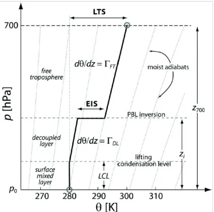
The 700 hPa level is chosen because it corresponds to the pressure at which an inversion is usually found as the air flows to the Equator from the subtropics. This bulk measure of the inversion strength has been used in different parameterization schemes for low level clouds, as high values of this parameter are usually associated to higher low cloud fractions. A recent work by Wood and Bretherton (2006) proposes an alternative measure that relates low cloud fraction to a more refined estimate of the inversion strength, which they termed Estimated Inversion Strength (EIS). This new estimate depends not only on the bulk LTS but it takes into account the detailed vertical structure of the lower tropospheric potential temperature profile (Figure 3).

The inversion at the PBL top is located a certain height with a strength , which normally ranges from 1-10 K. The PBL may be vertically well mixed or decoupled into multiple turbulent layers. This decoupling is usually modeled using a bulk scheme that breaks the PBL into a surface mixed layer, that extends from the surface up to the LCL and has constant ; and a decoupled layer that extends from the LCL up to the inversion level, where increases linearly with height at a rate . Above the inversion (in the

free troposphere), also increases linearly with height, at a rate . It is straightforward to relate the inversion strength to the LTS and these lapse rates:

( ) ( ) ( ) (2)

where is the height of the 700 hPa pressure level. This would perfectly correlate with the LTS (the first term on the rhs), provided that all the other terms are constant. However, it can be shown that they actually vary as a function of . In the Tropics the temperature profile is close to a moist adiabat, which is supported by the idea that due to the relatively weak Coriolis force, large horizontal temperature gradients are very unlikely (Wood and Bretherton, 2006), so the temperature profile is largely determined by the regions of deep convection at the ITCZ. Moreover, it was shown that is positively correlated to , which shows that the LTS alone cannot be the only

(23)

10

responsible for . On the other hand, the decoupled layer also shows some degree of dependency on surface properties, as its temperature profile is usually is approximated by the shape of moist adiabat that crosses the LCL (which may be determined as a function of surface properties alone). If it is assumed that the decoupled layer is usually much shallower than the free tropospheric layer below 700 hPa, and that , the

EIS may then be computed as:

( ) (3)

The latter relationship holds not only in tropical and subtropical regions (which were already satisfactorily explained by the LTS relationship) but also at the midlatitudes, as shown in Figure 4. Regions marked with “At” (North Atlantic) and “Pa” (North Pacific), collapse into the regression line using EIS which did not happen with the LTS relationship, that only holds in tropical and subtropical regions.

Figure 3 – Typical vertical structure of the potential temperature profile in a situation of undisturbed flow with moderate tropospheric subsidence. The gray lines are moist adiabats. From (Wood and Bretherton,

2006).

Global remote sensing observations of these parameters are possible using multi-sensor approaches, such as the one proposed by Yue et al. (2011). They used thirteen months of observations of temperature and water vapor from the Atmospheric InfraRed Sounder (AIRS) onboard Aqua, cloud profiles from the Cloud Profiling Radar (CPR) onboard

(24)

11

Cloudsat and Cloud-Aerosol Lidar with Orthogonal Polarization (CALIOP) onboard CALIPSO, which are part of NASA‟s A-Train (Stephens et al., 2002), a constellation of polar-orbiting satellites with orbits minutes apart from each other that provide complementary views of the same ground scene. These datasets were collocated with European Center for Medium-Range Forecasts (ECMWF) model analysis (non-collocated National Centers for Environmental Prediction (NCEP) National Centers for Atmospheric Research (NCAR) reanalysis data was also used for comparison). The authors focused on the characterization of stratocumulus decks, namely in the global estimation of parameters such as LTS and EIS. As expected, higher values of EIS are related to the presence of low clouds, as diagnosed by CloudSat. The comparison between both reanalyses revealed large discrepancies that were attributed to differences in model physics as well as to different temporal and spatial sampling. The use of CALIOP allowed the confirmation of the results shown in Figure 4 (on which a linear relationship between LTS/EIS and cloud fraction is derived), using global remote sensing data, and not only surface based cloud observations, as done by Wood and Bretherton (2006).

Figure 4 – Relationship between Low Cloud Fraction a) LTS and b) EIS using data from regions where low stratiform clouds are predominant according to Klein and Hartmann (1993). See text for details. From Wood

and Bretherton (2006).

The structure of the stratiform cloud decks is not homogeneous, as shown by the results from VOCALS-Rex (Bretherton et al., 2010). In the particular case of the Peruvian stratus deck, the clouds tend to be shallower close to land and the air above the inversion tends to be more humid, an effect of the ventilation caused by mountain breezes originating in the Andes. Offshore, the PBL is usually deeper and decoupled (e.g. Zuidema et al., 2009) and drizzle often occurs. The horizontal structure is also characterized by the presence of pockets of open cells. The transition between these two regimes is not well understood. Some studies suggest that LTS alone is not a suitable

(25)

12

indicator of the presence of low clouds out of the core of the stratocumulus regions, near the transition to the shallow cumulus region. Instead, cold advection seems to be more important (Klein, 1997), which suggests that the local cloud amount may be determined by the upstream conditions. This conclusion is supported by Pincus et al. (1997) who used satellite data to demonstrate the existence of significant correlations between images separated up to 24h in different locations of the Lagrangian trajectory the clouds perform on their way towards the tropics. The way these clouds later evolve to shallow cumuli is still a matter of debate. The traditional explanations rely on the fact that the

LTS is reduced as SST increases, increasing turbulence and favoring the cloud top

instability, which favors entrainment of free tropospheric air into the PBL, breaking the cloud decks.

2.4 Trade Wind Shallow Cumulus

Shallow cumulus may form everywhere on Earth, and are particularly common over the ocean, and over land in fair weather conditions. The trade wind belts are areas where this type of convection is favored due to their light subsidence rates and warm SSTs (when compared to the SSTs in the stratocumulus regions). Their importance in maintaining the overall tropical circulation has been recognized for a long time (e.g. Riehl et al., 1951). In these regions, a temperature inversion caps the PBL and inhibits further vertical development of the PBL clouds. It is generally weaker than the inversions found over stratocumulus decks.

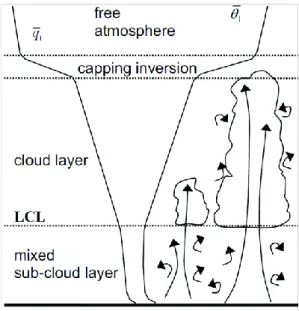
The typical structure of the PBL under shallow convection is depicted in Figure 5. The region closer to the ground is slightly unstable due to the underlying warming, favoring vertical updrafts. Some of them are strong enough to reach the LCL and form a cloud. Clouds usually occupy less than 10% of the horizontal area. The traditional view of the vertical transport in a shallow cumulus cloud layer employs the notion that there cloudy updrafts that occupy a relatively small area which are compensated by a slowly subsiding environment. There are recent studies using LES that show that a large part of the downward vertical transport is actually done by narrow subsiding shells around the cumulus clouds, that form when cloudy air detrains from the cloud and evaporates, becoming negatively buoyant (Heus and Jonker, 2008; Jonker et al., 2008). At the top of the turbulent layer, there is an inversion which may extend up to a few hundred meters above the cloud top.

(26)

13

Figure 5 – The typical vertical structure of a shallow convective PBL. from Soares et al. (2004).

Neggers et al. (2007) demonstrated the importance of shallow convection to tropical climate. They used a simplified tropical circulation model, the Quasi-equilibrium Tropical Circulation Model (Neelin and Zeng, 2000) and varied the intensity of the subtropical shallow cumulus convective mixing through the adjustment of the shallow convective adjustment time scale, . They found that due to a decrease of shallow cumulus activity, the tropical evaporation and temperature decrease. This sensitivity is explained by a somewhat complex feedback mechanism (Figure 6). The reduction of the mixing due to less active shallow convective clouds decreases the amount of water vapor that is transported from the PBL to the lower free troposphere. Locally, the PBL will then retain that extra moisture and the surface evaporation is reduced, so a local energy imbalance occurs, which has to be compensated. The relatively dry air just above the PBL is transported by the trade winds towards the Equator, where it plays an important role in the onset of deep convective towers at the ITCZ. As shown by Derbyshire et al. (2004) with Cloud Resolving Model (CRM) simulations, deep convection is very sensitive to the mid-tropospheric humidity, so a reduction of moisture transported towards the Equator results in an inhibition of deep convection at the edges of the ITCZ and consequently in a narrowing of this region. The decrease in latent heat release due to suppressed convection will cause a temperature drop in the whole tropics by a few degrees. This has a significant radiative impact, as the longwave radiation emission will decrease, along with a slight increase of the surface heat flux. In the core of the ITCZ, the situation is slightly different: the net radiation is positive there and the convection is actually strengthened, helped by a stronger surface convergence

(27)

14

(associated to the equatorial convergence of the trade wind belts), increasing precipitation and surface evaporation.

Figure 6 – Illustration of the mechanisms leading to the sensitivity of the strength of the tropical general circulation to the evaporation caused by trade wind shallow cumulus. From Neggers et al. (2007).

2.5 Deep convection

Near the Equator, the Sun zenithal angle is minimum, so the amount of direct radiation that reaches the top of the atmosphere is greater there than in any other region in the planet. The impacts of the solar radiation on the atmosphere are indirect and depend on the surface characteristics. Ocean areas store heat more efficiently than land areas, not only due to the larger heat capacity of water, when compared to heat capacities of land surfaces, but also due to the mixing on the oceanic boundary layer. The surface re-emits the energy it receives from the Sun in the form of surface turbulent fluxes of heat and moisture. The partition between both is different depending on surface type and affects the way convection develops during the diurnal cycle.

The ocean areas where deep convection occurs are characterized by high SSTs (generally warmer than 27-28ºC), convergent surface winds and high relative humidity (e.g. Bretherton et al., 2004; Derbyshire et al., 2004). The atmosphere in these regions is also characterized by high values of CAPE (Riemann-Campe et al., 2009). This concept has been used as a closure for the majority of the cumulus convection parameterization schemes (e.g., Arakawa, 2004 and references therin). It is defined as the vertical integral

(28)

15

of the positive departure of the temperature profile with respect to the temperature profile that a rising air parcel would have if it was lifted through a moist adiabatic process from the surface (Emanuel, 1994). Deep convection occurs as PBL air parcels become able to overcome the Convective Inhibition (CIN) – the amount of energy needed by an air parcel to reach the Level of Free Convection (LFC), i.e. the height where the temperature of the moist adiabatic process becomes greater than the environmental profile. Only a few plumes have enough energy to overcome this layer, so the more turbulence there is in the PBL, the more turbulent plumes are likely to become deep cumulus clouds. The local effects of deep convection are twofold: it dries and warms the atmosphere where it occurs. The drying happens more intensely below the freezing level (at about 5km), whereas the warming occurs at upper levels. This is consistent with the co-existence of two modes of convection in these areas: shallow non-precipitating and deep precipitating. In fact, convective towers tend to self-organize in cloud clusters and sometimes into rather large mesoscale convective systems. The surroundings of these systems are usually characterized by the presence of shallow cumuli (that may later develop into congestus) or regions of stratiform clouds - which may also produce large amounts of precipitation, or even no clouds at all, such as in the case of what happens in the cold pools produced by the evaporation of precipitation from the convective towers (Khairoutdinov and Randall, 2006). Precipitation comes from these deep convective clouds, but also from the stratiform regions in equal parts, despite the fact that the intensity of individual showers is much larger (by a factor of four or greater; Schumacher and Houze, 2003).

Nesbitt and Zipser (2003) discussed some of the differences of the deep convection diurnal cycle over land and over the ocean. Its amplitude is much larger over land surfaces, with maximum rainfall in the afternoon due to stronger solar irradiation and boundary layer destabilization. There are certain regions where local convection is reinforced by sea-breeze and complex terrain circulations or even by the occurrence of mesoscale convective systems, leading to maximum rainfall a few hours later during the night. Over the oceans, there are a few studies pointing to the strong influence of remote forcing from nearby land regions through gravity waves or coastline effects (Rahn and Garreaud, 2010). In regions that are not close enough to land masses, there is some degree of debate on the causes of the observed diurnal cycle. Possible mechanisms include 1) the differential radiative heating between convective and the surrounding

(29)

16

cloud-free region producing a daily variation in the horizontal divergence field that modulates convection; 2) the minimum in the morning precipitation may be related to the absorption of shortwave radiation by the upper portions of the cloud anvils, which increases static stability and inhibits vertical motions; conversely, in the night longwave cooling in clouds decreases stability and increases the strength of the convection; 3) the increase in relative humidity at night due to longwave cooling reduces the effects of entrainment and enhances cloud development; 4) more complex and debatable mechanisms such as the occurrence of a maximum in ocean skin temperature in late afternoon, consequent enhanced convection during the night and reduction in the morning due to depletion of moist static energy in the wakes produced by convection and shading of the ocean by deeper clouds. These mechanisms may act altogether, since it is very difficult to isolate their individual action in currently available datasets (Nesbitt and Zipser, 2003). The representation of the diurnal cycle of deep convection has been a major challenge in the numerical weather prediction and climate modeling communities and will be further discussed in chapter 3.

2.6 The GCSS/WGNE Pacific Cross-section Intercomparison

(GPCI)

The need to better understand the physics and dynamics of clouds and to improve the parameterizations of clouds and cloud-related processes in weather and climate prediction models led to the creation of the Global Energy and Water Cycle Experiment (GEWEX) Cloud Systems Study (GCSS) in the early 1990s (Browning et al. 1993; Randall et al. 2003). Research efforts in GCSS have been divided into different cloud types: boundary layer clouds, cirrus, frontal clouds, deep convection, and polar clouds. The GCSS community has extensively used LES and CRMs to assess those models‟ ability to describe clouds, through the development and evaluation of parameterizations for single column models (SCM), which are one-dimensional versions of weather and climate prediction models.

The traditional GCSS strategy can be divided in the following steps: (i) create a case study using observations; (ii) evaluate CRM/LES models for the case study; (iii) use SCMs to evaluate the parameterizations; and (iv) use the statistics from CRM/LES to develop and improve parameterizations. This strategy has been quite successful in improving CRM/LES models, in helping to define and understand fundamental cloud

(30)

17

regimes (e.g. Bretherton et al., 1999; Bechtold et al., 2000; Redelsperger et al., 2000; Duynkerke and Teixeira, 2001; Stevens et al., 2001; Randall et al., 2003) and in developing new parameterizations for clouds and the cloudy boundary layer (e.g. Cuijpers and Bechtold, 1995; Lock et al., 2000; Golaz et al., 2002; Teixeira and Hogan, 2002; Cheinet and Teixeira, 2003; Lenderink et al., 2004; McCaa and Bretherton, 2004; Soares et al., 2004; Bretherton and Park, 2009).

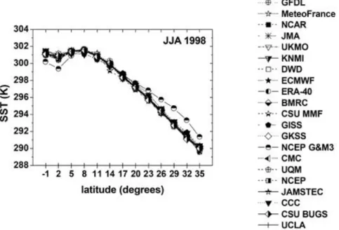
The convection regimes described above predominantly occur in certain regions where the environmental characteristics favor their maintenance. In the East Pacific Ocean the large scale circulation advects air masses that form off the west coast of California towards the Equator along the trade wind streamlines. In their trajectory, the environmental conditions change quite dramatically: SST changes from 290 K off the coast of California to 302K in the Equator – see Figure 10, and the subsidence rates also change rather severely. As a consequence, transitions between convection regimes occur. Stratocumulus decks turn into broken stratocumulus, which then evolve to shallow cumulus and finally deep cumulus convection occurs at the ITCZ. Teixeira et al. (2011) reviewed some of the deficiencies in the representation of these transitions by comparing the results from 20 models from different climate and weather prediction centers, satellite observations and ECMWF reanalysis in an transection in the East Pacific, designed to coincide with the trade wind streamlines and to be representative of the large scale circulation and of the transition between the different convection regimes. The transect consists of 13 locations ranging from (35ºN, 125ºW) in the northeast to (1ºS, 173ºW) in the southwest, with steps of 4º longitude and 3º latitude (Figure 7). Preliminary studies using a similar cross section across the Pacific Ocean were performed in the context of a European Union Project on Cloud Systems (EUROCS). While important, the EUROCS results (Siebesma et al., 2004) were limited due to coarse temporal resolution (only monthly mean values at four different times per day were available) and the absence of some critical observational data sources for the evaluation of the model results, such as information about the tropospheric temperature and humidity structure. In the course of the work discussed here, three-hourly model output from the simulations of the periods of June-August 1998 and 2003 over the GPCI transect were compiled, as well as two-dimensional fields of certain variables for completeness. This temporal frequency allows a better characterization of diurnal variability. One of the questions that the use of such an idealized framework raises is

(31)

18

how representative is the GPCI transect of the processes that characterize the convection regimes and transitions between them. It is assumed that there is an alignment between the transect orientation and the trajectories described by the air masses. Mean boundary layer wind directions from ERA-40, for June-August 1998 are shown to roughly coincide with the orientation of the transect (see Figures 2 and 3 of Teixeira et al., 2011). That may not necessarily be the case for some of the models used in the intercomparison, but it is shown that they indeed exhibit bulk Hadley circulation characteristics using alternative diagnostics.

Figure 7 – Location of the GPCI transect, overlayed on contours of International Satellite Cloud Climatology Project (ISCCP) low cloud fraction (adapted from Karlsson et al., 2010).

The 2D dataset mentioned above is used to investigate the representativity of the transect. Histograms of variables, like total cloud cover (TCC) and precipitation, along the GPCI transect are compared to longitudinally adjacent points (5 degrees to the east and to the west). Figure 8 shows the histograms of precipitation for one GPCI point (5ºN, 195ºE) and the two adjacent points from the GFDL, and NCAR models for the period of JJA 1998. Figure 9 shows a similar plot but for the TCC and another GPCI point - 20ºN, 215ºE. It is clear from these figures that the histograms for both TCC and precipitation are quite similar between adjacent points for the same model and quite different between models. Similar results are obtained for different points along the GPCI transect as well as for different models (not shown). Overall, these results support the idea that GPCI is sufficiently representative for the purposes of this study of the main model physical processes of the subtropics in this region.

(32)

19

Figure 8 – Histogram of precipitation (mm day-1) from the National Centers for Atmospheric Research (NCAR) and Geophysical Fluid Dynamics Laboratory (GFDL) models for one GPCI point (5ºN, 195ºE) and two adjacent (5º to the east and west along the same latitude) points for JJA 1998. From Teixeira et al. (2010).

Figure 9 – Histogram of total cloud cover (TCC) (%) from the NCAR and GFDL models for one GPCI point (20ºN, 215ºE) and two adjacent (5º to the east and west along the same latitude) points for JJA 1998. From

Teixeira et al. (2010).

The models, observations and reanalysis were compared using several diagnostics along the transect, which included SSTs (shown in Figure 10), total column water vapor, outgoing longwave radiation, as well as vertical cross-sections of subsidence, relative

(33)

20

humidity, cloud fractions and cloud liquid water content. In general, the results showed large spreads in the representation of clouds and cloud-related processes. Even reanalysis such as ERA-40 show strong inconsistencies with observations. In the case of SSTs (Figure 10), all models except NCAR G&M (National Centers for Atmospheric Research – Global Forecast System and Modular Ocean Model version 3, the only atmosphere and ocean coupled model used in the comparison) show similar distributions along the GPCI transect. The differences between the uncoupled models are mainly explained by the use of different implementations for describing the SSTs, such as the use of different analysis. The differences in the representation of the other atmospheric variables are mostly related to the differences in the physical parameterizations used in each model to represent subgrid scale processes. Even ERA-40 suffers from serious biases in some of those variables: it was shown that when compared to International Satellite Cloud Climatology Project (ISCCP) observations, ERA-40 cloud cover is negatively biased in the stratocumulus regions. This is partially explained by the fact that it does not directly assimilate cloud-related variables from observations. Those biases have been recently improved in ERA-Interim by the inclusion of an eddy-diffusivity mass-flux approach, adapted to represent stratocumulus regimes (Köhler et al., 2011). The bias is also present in the majority of the models in terms of liquid water path (when compared to SSM/I observations), which in turn is reflected in positive shortwave radiation biases at the surface and at the top of the atmosphere. In the deep tropics, ERA-40 (in particular) overestimates cloud cover, liquid water path, precipitation and, as a consequence, underestimates the outgoing longwave radiation.

(34)

21

Figure 10 – Sea Surface Temperature (K) along GPCI for JJA 1998 for all the models in the intercomparison. See Teixeira et al. (2011) for details on the models.

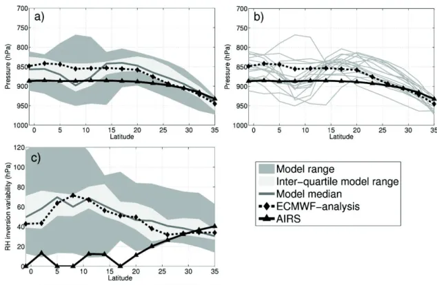
In a complementary work, Karlsson et al. (2010) discussed the variability of cloud top heights along the GPCI transect, which in regions of extensive low level cloudiness is well correlated with PBL height (e.g., Zuidema et al., 2009). The same framework in Teixeira et al. (2011) was used, and comparisons against different remote sensing instruments were performed, such as against the Atmospheric Infrared Sounder (AIRS) and the Multiangle Imaging SpectroRadiometer (MISR), but using the data for June-August 2003. The relative humidity profiles along the transect were used to estimate the level of the RH inversion, defined as the level where the RH gradient with respect to pressure is largest, below 700 hPa. Results from the models were compared to the AIRS V5 L2 Standard product (an earlier version of the product used in the subsequent chapters).

Figure 11 presents the analysis of the PBL heights variability in the GPCI transect, as given by the different models, ECMWF analysis and AIRS. The top left plot shows the general growth of the PBL from the stratocumulus regions to the Equator which is relatively consistent in all the models in the subtropics, but with large disagreement in the tropical region, showing inter model spreads of the order of the PBL height (top right plot of Figure 11). AIRS shows too little temporal and spatial variability, which is probably caused by the low vertical resolution of the used product. It should be mentioned that in the tropics the definition of PBL height is somewhat ambiguous, since there is relatively weak subsidence when compared to the subtropical regions, making

(35)

22

the inversions very weak, if they exist, and difficult to detect. ECMWF analysis always overestimates PBL heights when compared to AIRS, but the values are almost always within the interquartile range. A follow-up of these results will be presented in chapter 5, since new products have become available since this study was produced.

Figure 11 - JJA 2003 PBL height estimate based on the pressure at the main RH inversion (below 700 hPa) as a function of latitude. (a) Mean values: the solid dark-gray line represents the median-model ensemble value, the light-gray envelope is the interquartile model range, and the dark-gray envelope represents the full range of the model values. (b) Mean values: individual models. (c) Temporal variability: 1 standard deviation. AIRS and the ECMWF analysis are represented by a triangle-marked solid black line and a diamond-marked black

(36)

23

3. Evolution of cloud structures in the transition from

shallow to deep convection over land

Abstract

The transition from shallow to deep convection is a crucial process in the life cycle of convection over land. The process is of paramount importance in tropical forest climate, where intense rain is produced on a daily basis during the rainy season, with very well established timings. However, its representation is deficient in the majority of GCMs, which tend to simulate maxima of precipitation too early in the morning, when compared to observations. In this work, high resolution cloud-resolving simulations of the onset of Amazonian deep convection are analyzed to assess the ability of the model to reproduce observed precipitation characteristics and its sensitivity to horizontal resolution and to the evaporation of precipitation. It is shown that simulations running at different resolutions produce significantly different results, with the higher resolution experiments experiencing a significantly slower build-up of deep convection and precipitation, implying that these simulations to not attain peak values in the given simulation time. Because of the previous result, the impact of evaporation and cold-pool dynamics is still tentative, although it is clearly present in some diagnostics. Finally, an analysis of length scales is proposed using separate algorithms to analyze turbulent length scales and cloud sizes in the three simulations.