Accurate High Performance Concrete Prediction with an Alignment-Based Genetic Programming System

ORIGINAL ARTICLE

Accurate High Performance Concrete

Prediction with an Alignment-Based Genetic

Programming System

Leonardo Vanneschi

_{, Mauro Castelli}

_{, Kristen Scott}

_{and Aleš Popovič}

Abstract

In 2013, our research group published a contribution in which a new version of genetic programming, called Geo-metric Semantic Genetic Programming (GSGP), was fostered as an appropriate computational intelligence method for predicting the strength of high-performance concrete. That successful work, in which GSGP was shown to outper-form the existing systems, allowed us to promote GSGP as the new state-of-the-art technology for high-peroutper-formance concrete strength prediction. In this paper, we propose, for the first time, a novel genetic programming system called Nested Align Genetic Programming (NAGP). NAGP exploits semantic awareness in a completely different way compared to GSGP. The reported experimental results show that NAGP is able to significantly outperform GSGP for high-performance concrete strength prediction. More specifically, not only NAGP is able to obtain more accurate pre-dictions than GSGP, but NAGP is also able to generate predictive models with a much smaller size, and thus easier to understand and interpret, than the ones generated by GSGP. Thanks to this ability of NAGP, we are able here to show the model evolved by NAGP, which was impossible for GSGP.

Keywords: high performance concrete, strength prediction, artificial intelligence, genetic programming, semantic awareness

© The Author(s) 2018. This article is distributed under the terms of the Creative Commons Attribution 4.0 International License (http://creat iveco mmons .org/licen ses/by/4.0/), which permits unrestricted use, distribution, and reproduction in any medium, provided you give appropriate credit to the original author(s) and the source, provide a link to the Creative Commons license, and indicate if changes were made.

1 Background

Concrete is a material mainly used for the construction of buildings. It is made from a mixture of broken stone or gravel, sand, cement, water and other possible aggregates, which can be spread or poured into moulds and forms a stone-like mass on hardening. Many different possible formulas of mixtures exist, each of which provides dif-ferent characteristics and performance, and concrete is nowadays one of the most commonly used human-made artifacts (Lomborg 2001). Some of the concrete mixtures commonly used in the present days can be very complex, and the choice of the appropriate mixture depends on the objectives that the project needs to achieve. Objec-tives can, for instance, be related to resistance, aesthetics

and, in general, they have to respect local legislations and building codes. As usual in Engineering, the design begins by establishing the requirements of the concrete, usually taking into account several different features. Typically, those features include the weather condi-tions that the concrete will be exposed to, the required strength of the material, the cost of the different aggre-gates, the facility/difficulty of the mixing, the placement, the performance, and the trade-offs between all these characteristics and possibly many others. Subsequently, mixtures are planned, generally using cement, coarse and fine aggregates, water and other types of components. A noteworthy attention must also be given to the mixing procedure, that has to be clearly defined, together with the conditions the concrete may be employed in. Once all these things are clearly specified, designers can finally be confident that the concrete structure will perform as expected. In the recent years, in the concrete construc-tion industry, the term high-performance concrete (HPC) has become important (Yeh 1998). Compared to

Open Access

*Correspondence: lvanneschi@novaims.unl.pt

1 _{NOVA Information Management School (NOVA IMS), Universidade Nova}

de Lisboa, Campus de Campolide, 1070-312 Lisbon, Portugal Full list of author information is available at the end of the article Journal information: ISSN 1976-0485 / eISSN 2234-1315

conventional concrete, HPC usually integrates the basic ingredients with supplementary cementitious materi-als, including for instance fly ash, blast furnace slag and chemical admixture, such as superplasticizer (Kumar et al. 2012). HPC is a very complex material, and mod-eling its behavior is a very hard task.

In the past few years, an extremely insightful result appeared, known as Abrams’ water-to-cement ratio (w/c) law (Abrams 1927; Nagaraj and Banu 1996). This law establishes a relationship between the concrete’s strength and the w/c ratio, basically asserting that the concrete’s strength varies inversely with the w/c ratio. One of the consequences is that the strengths of different concretes are identical as long as their w/c ratios remain the same, regardless of the details of the compositions. The impli-cations of the Abrams’ rule are controversial and they have been the object of a debate for several years. For instance, one of these implications seems to be that the quality of the cement paste controls the strength of the concrete. But an analysis of a variety of experimental data seems to contradict this hypothesis (Popovics 1990). For instance, in Popovics (1990) it is demonstrated that if two concrete mixtures have the same w/c ratio, then the strength of the concrete with the higher cement con-tent is lower. A few years later, several studies have inde-pendently demonstrated that the concrete’s strength is determined not only by the w/c ratio, but also by other ingredients [see for instance (Yeh 1998; Bhanja and Sen-gupta 2005)], In conclusion, the Abrams’ law is nowadays considered as practically acceptable in many cases, but a few significant deviations have been reported. Currently, empirical equations are used for estimating the concrete strength. These equations are based on tests that are usu-ally performed without further cementitious materials. The validity of these relationships for concrete in case of presence of supplementary cementitious materials (like for instance fly ash or blast furnace slag) is nowadays the object of investigation (Bhanja and Sengupta 2005). All these aspects highlight the need for reliable and accu-rate techniques that allow modeling the behavior of HPC materials.

To tackle this problem, Yeh and Lien (2009) proposed a novel knowledge discovery method, called Genetic Operation Tree (GOT), which consists in a composition of operation trees (OT) and genetic algorithms (GA), to automatically produce self-organized formulas to predict compressive strength of HPC. In GOT, OT plays the role of the architecture to represent an explicit formula, and GA plays the role of the mechanism to optimize the OT to fit experimental data. The presented results showed that GOT can produce formulas which are more accu-rate than nonlinear regression formulas but less accuaccu-rate than neural network models. However, neural networks

are black box models, while GOT can produce explicit formulas, which is an important advantage in practical applications.

A few years later, Chou et al. (2010) presented a com-parison of several data mining methods to optimize the prediction accuracy of the compressive strength of HPC. The presented results indicated that multiple additive regression tree (MART) was superior in prediction accu-racy, training time, and aversion to overfitting to all the other studied methods.

Cheng et  al. (2013) asserted that traditional methods are not sufficient for such a complex application as the optimization of prediction accuracy of the compressive strength of HPC. In particular, they identified important limitations of the existing methods, such as their expen-sive costs, their limitations of use, and their inability to address nonlinear relationships among components and concrete properties. Consequently, in two different contributions, Cheng and colleagues introduced novel methods and applied them to this type of application. In Cheng et  al. (2013), they introduced a novel GA— based evolutionary support vector machine (called GA-ESIM), which combines the K-means and chaos genetic algorithm (KCGA) with the evolutionary support vec-tor machine inference model (ESIM), showing interest-ing results. In Cheng et  al. (2014), they introduced the Genetic Weighted Pyramid Operation Tree (GWPOT). GWPOT is an improvement of Yeh and Lien’s GOT method (Yeh and Lien 2009), and it was shown to out-perform several widely used artificial intelligence models, including the artificial neural network, support vector machine, and ESIM.

In the same research track, in 2013 our research group investigated for the first time the use of Genetic Pro-gramming (GP) (Poli et al. 2008; Koza 1992) as an appro-priate technology for predicting the HPC strength. GP is a computational intelligence method aimed at evolving a population of programs or individuals (in our case, pre-dictive models for the HPC strength) using principles inspired by the theory of evolution of Charles Darwin. Basilar to GP is the definition of a language to code the programs and a function, called fitness, that for each pos-sible program quantifies its quality in solving the prob-lem at hand (in our case, the probprob-lem of predicting the HPC strength). Fitness is often calculated by running the program on a set of data (usually called training instances, or training cases) and quantifying the differ-ence between the behaviour of the program on those data and the (known) expected behaviour. It is a recent trend in the GP research community to develop and study methods to integrate semantic awareness in this evolu-tionary process, where with the term semantics we gen-erally indicate the vector of the output values calculated

by a model on all the available training cases. Our work from 2013 (Castelli et  al. 2013) clearly indicated that a relatively recent and sophisticated version of GP, that exploits semantic awareness, called Geometric Seman-tic GP (GSGP) (Moraglio et al. 2012; Vanneschi 2017) is able to outperform standard GP, predicting HPC strength with high accuracy. This success motivated us to pursue the research, with the objective of further improving the results obtained by GSGP, possibly investigating new and more promising ways of exploiting semantic awareness. The contribution of this work is twofold:

• In the first place, we deepen a very recent and prom-ising idea to exploit semantic awareness in GP, called alignment in the error space (Ruberto et  al. 2014), that received relatively little attention by the GP com-munity so far;

• Secondly, we define a novel computational intelli-gence method, called Nested Align Genetic Program-ming (NAGP), based on the concept of alignment in the error space, that is able to outperform GSGP for HPC strength prediction.

The former contribution is important for the GP com-munity because it represents a further step forward in a very popular research line (improving GP with semantic awareness). On the other hand, considering that GSGP is regarded as the state-of-the-art computational tech-nology for HPC strength prediction, the latter contribu-tion promises to have a tremendous impact on this very important applicative domain.

As we will see in the continuation of this paper, NAGP has two competitive advantages compared to GSGP: not only NAGP is able to obtain more accurate predictive models for the HPC strength, but these models are also smaller in size, which makes them more readable and interpretable. This last characteristic is very important in a complex application such as the HPC strength predic-tion. In fact, the dimension of the model is clearly con-nected with the ability of users to understand the model.

The paper is organized as follows: Sect. 2 contains a gentle introduction to GP, also offering pointers to bib-liographic material for deepening the subject. Section 3 introduces GSGP, motivating the reasons for its recent success. In Sect. 4, we introduce the idea of alignment in the error space, also discussing some previous pre-liminary studies in which this idea was developed. In Sect. 5, we present for the first time NAGP and a variant of NAGP called NAGP_β, motivating every single step of their implementation. In Sect. 6, we describe the data and the experimental settings and we present and discuss the obtained experimental results, comparing the perfor-mance of NAGP and NAGP_β to the one of GSGP for the

HPC strength prediction. Finally, Sect. 7 concludes the paper and proposes suggestions for future research.

2 An Introduction to Genetic Programming

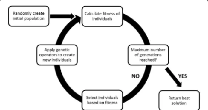
Genetic Programming (GP) (Koza 1992) is a computa-tional method that belongs to the computacomputa-tional intel-ligence research area called evolutionary computation (Eiben and Smith 2003). GP consists of the automated learning of computer programs by means of a process inspired by the theory of biological evolution of Darwin. In the context of  GP, the word program can be inter-preted in general terms, and thus GP can be applied to the particular cases of learning expressions, functions and, as in this work, data-driven predictive models. In GP, programs are typically encoded by defining a set  F of primitive functional operators and a set  T of termi-nal symbols. Typical examples of primitive functiotermi-nal operators may include arithmetic operations (+, −, *, etc.), other mathematical functions (such as sin, cos, log, exp), or, according to the context and type of prob-lem, also boolean operations (such as AND, OR, NOT), or more complex constructs such as conditional operations (such as If–Then-Else), iterative operations (such as While-Do) and other domain-specific functions that may be defined. Each terminal is typically either a vari-able or a constant, defined on the problem domain. The objective of GP is to navigate the space of all possible programs that can be constructed by composing sym-bols in F and T, looking for the most appropriate ones for solving the problem at hand. Generation by generation, GP stochastically transforms populations of programs into new, hopefully improved, populations of programs. The appropriateness of a solution in solving the problem (i.e. its quality) is expressed by using an objective func-tion (the fitness funcfunc-tion). The search process of GP is graphically depicted in Fig. 1.

In order to transform a population into a new pop-ulation of candidate solutions, GP selects the most

promising programs that are contained in the current population and applies to those programs some particu-lar search operators called genetic operators, typically crossover and mutation. The standard genetic opera-tors (Koza 1992) act on the structure of the programs that represent the candidate solutions. In other terms, standard genetic operators act at a syntactic level. More specifically, standard crossover is traditionally used to combine the genetic material of two parents by swapping a part of one parent with a part of the other. Consider-ing the standard tree-based representation of programs often used by GP (Koza 1992), after choosing two indi-viduals based on their fitness, standard crossover selects a random subtree in each parent and swaps the selected subtrees between the two parents, thus generating new programs, the offspring. On the other hand, standard mutation introduces random changes in the structures of the individuals in the population. For instance, the tradi-tional and commonly used mutation operator, called sub-tree mutation, works by randomly selecting a point in a tree, removing whatever is currently at the selected point and whatever is below the selected point and inserting a randomly generated tree at that point. As we clarify in Sect. 3, GSGP (Moraglio et al. 2012; Vanneschi 2017) uses genetic operators that are different from the stand-ard ones, since they are able to act at the semantic level. The reader who is interested in deepening GP is referred to Poli et al. (2008) and Koza (1992).

2.1 Symbolic Regression with Genetic Programming The prediction of HPC strength is typically a symbolic regression problem. So, it is appropriate to introduce here the general idea of symbolic regression and the way in which this kind of problem is typically approached with GP. In symbolic regression, the goal is to search for the symbolic expression TO_:Rp_{→R that best fits a}

par-ticular training set T = {(x1, t1), . . . , (xn, tn)} of n input/

output pairs with xi ∈Rp and ti∈R . The general

sym-bolic regression problem can then be defined as:

where G is the solution space defined by the primitive set (functions and terminals) and f is the fitness function, based on a distance (or error) between a program’s out-put  T(xi) and the expected, or target, output  ti . In other

words, the objective of symbolic regression is to find a function  TO _{(called data model) that perfectly matches}

the given input data into the known targets. In symbolic regression, the primitive set is generally composed of a set of functional symbols F containing mathematical functions (such as, for instance, arithmetic functions, trigonometric functions, exponentials, logarithms, etc.)

(1)

To←arg minT ∈Gf (T (xi), ti) with i = 1, 2, . . . , n

and by a set of terminal symbols T containing p vari-ables (one variable for each feature in the dataset), plus, optionally, a set of numeric constants.

3 Geometric Semantic Genetic Programming

Even though the term semantics can have several dif-ferent interpretations, it is a common trend in the GP community (and this is what we do also here) to identify the semantics of a solution with the vector

s(T ) = [T (x1), T (x2), . . . , T (xn)] of its output values on

the training data (Moraglio et al. 2012; Vanneschi et al. 2014). From this perspective, a GP individual can be identified by a point [its semantics s(T)] in a multidimen-sional space that we call semantic space (where the num-ber of dimensions is equal to the numnum-ber of observations in the training set, or training cases). The term Geomet-ric Semantic Genetic Programming (GSGP) (Vanneschi 2017) indicates a recently introduced variant of GP in which traditional crossover and mutation are replaced by so-called Geometric Semantic Operators (GSOs), which exploit semantic awareness and induce precise geomet-ric properties on the semantic space. GSOs, introduced by Moraglio et al. (2012), are becoming more and more popular in the GP community (Vanneschi et  al. 2014) because of their property of inducing a unimodal error surface (characterized by the absence of locally optimal solutions on training data) on any problem consisting of matching sets of input data into known targets (like for instance supervised learning problems such as sym-bolic regression and classification). The interested reader is referred to (Vanneschi 2017) for an introduction to GSGP where the property of unimodality of the error surface is carefully explained. Here, we report the defini-tion of the GSOs as given by Moraglio et al. for real func-tions domains, since these are the operators we will use in this work. For applications that consider other types of data, the reader is referred to Moraglio et al. (2012).

Geometric semantic crossover generates, as the unique

offspring of parents T1, T2, the expression:

where TR is a random real function whose output values

range in the interval [0,1]. Analogously, geometric

seman-tic mutation returns, as the result of the mutation of an

individual T : Rn_{→R , the expression:}

where TR1 and TR2 are random real functions with

codo-main in [0,1] and ms is a parameter called mutation step. Moraglio and co-authors show that geometric seman-tic crossover corresponds to geometric crossover in the semantic space (i.e. the point representing the offspring stands on the segment joining the points representing the

(2)

TXO= (T1·TR) + ((1 − TR) ·T2)

(3)

parents) and geometric semantic mutation corresponds to box mutation on the semantic space (i.e. the point representing the offspring stands into a box of radius ms, centered in the point representing the parent).

As Moraglio and co-authors point out, GSGP has an important drawback: GSOs create much larger offspring than their parents and the fast growth of the individu-als in the population rapidly makes fitness evaluation unbearably slow, making the system unusable. In Castelli et al. (2015), a possible workaround to this problem was proposed by our research team, consisting in an imple-mentation of Moraglio’s operators that makes them not only usable in practice, but also very efficient. With this implementation, the size of the individuals at the end of the evolution is still very large, but they are represented in a particularly clever way (using memory pointers and avoiding repetitions) that allows us to store them in memory efficiently. So, using this implementation, we are able to generate very accurate predictive models, but these models are so large that they cannot be read and interpreted. In other words, GSGP is a very effective and efficient “black-box” computational method. It is the implementation introduced in Castelli et  al. (2015) that was used with success in Castelli et al. (2013) for the pre-diction of HPC strength. One of the main motivations of the present work is the ambition of generating predictive models for HPC strength that could have the same per-formance as the ones obtained by GSGP in Castelli et al. (2013), or even better if possible, but that could also have a much smaller size. In other words, while still having very accurate predictive models for the HPC strength, we also want models that are readable and interpretable.

4 Previous Work on Alignment in the Error Space

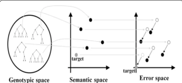
Few years after the introduction of GSGP, a new way of exploiting semantic awareness was presented in Ruberto et al. (2014) and further developed in Castelli et al. (2014) and Gonçalves et al. (2016). The idea, which is also the focus of this paper, is based on the concept of error space, which is exemplified in Fig. 2.

In the genotypic space, programs are represented by their syntactic structures [for instance trees as in Koza (1992), or any other of the existing representations]. As explained above, semantics can be represented as a point in a space that we call semantic space. In supervised learning, the target is also a point in the semantic space, but usually (except for the rare case where the target value is equal to zero for each training case) it does not correspond to the origin of the Cartesian system. Then, we translate each point in the semantic space by subtract-ing the target from it. In this way, for each individual, we obtain a new point, that we call error vector, and we call the corresponding space error space. The target, by

construction, corresponds to the origin of the Cartesian system in the error space. In Ruberto et  al. (2014), the concepts of optimally aligned, and optimally coplanar, individuals were introduced, together with their impor-tant implications that are summarized here.

Two individuals A and B are optimally aligned if a sca-lar constant k exists such that

where →_e

A and →eB are the error vectors of A and B

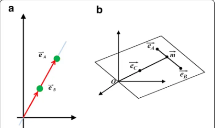
respectively. From this definition, it is not difficult to see that two individuals are optimally aligned if the straight line joining their error vectors also intersects the origin in the error space. This property is graphically shown in Fig. 3a. Analogously, and extending the idea to three dimensions, three individuals are optimally coplanar if the bi-dimensional plane in which their error vectors lie in the error space also intersects the origin. This property is shown in Fig. 3b.

In Ruberto et al. (2014), it is proven that given any pair of optimally aligned individuals A and B, it is possible to reconstruct a globally optimal solution Popt . This solution

is defined in Eq. (3):

where k is the same constant as in Eq. (2). This optimal solution is represented in a tree shape in Fig. 4.

Analogously, in Ruberto et al. (2014), it was also proven that given any triplet of optimally coplanar individuals, it is possible to analytically construct a globally optimal solution [the reader is referred to Ruberto et al. (2014) for the equation of the globally optimal solution in that case]. As Fig. 3b shows, the three-dimensional property is just an extension of the bi-dimensional one; in fact, if three individuals A, B and C are optimally coplanar, it is always possible to find a vector →_{m that is aligned with} →_e

A and →_e

B and that is also aligned with →eC and the origin.

Several possible ways of searching for alignments can be imagined. In Ruberto et  al. (2014), one first

(4) →_e A=k ·→eB (5) Popt= 1 1 − kA − k 1 − kB

preliminary attempt was made by fixing one direction, called attractor, and “pushing” all the individuals in the population towards an alignment with the attractor. In this way, it is possible to maintain the traditional repre-sentation of solutions where each solution is represented by one program. The other face of the coin is that, in this way, we strongly restrict what GP can do, forcing the alignment to necessarily happen in just one prefixed direction, i.e. the one of the attractor. The objective of this paper is to relieve this constraint by defining a new GP system that is generally able to evolve vectors of pro-grams (even though only vectors of size equal to 2 will be used in this paper).

In Castelli et al. (2014), a first attempt of using a mul-tiple program representation was made. In that work, individuals were pairs of programs, and fitness was the angle between the respective error vectors. This situation is graphically represented in Fig. 5, where the two error vectors are called →_{a and} →_{b and the angle used as}

fit-ness is called ϑ. It is obvious that if ϑ is equal to zero, then

→_{a and} →_{b are aligned between each other and with the}

origin. Thus, the objective of GP is to minimize ϑ.

In this way, alignments could be found in any possible direction of the error space, with no restrictions. From

now on, for the sake of clarity, this type of individual (i.e. individuals characterized by more than one program) will be called multi-individuals. In Castelli et al. (2014), the following problems of this approach were reported:

• Generation of semantically identical, or very similar, expressions;

• k constant in Eq. (3) equal, or very close, to zero; • Generation of expressions with huge error values. These problems strongly limited the work, at the point that the approach itself was considered as unusable in practice in Castelli et al. (2014). These problems are dis-cussed here, while in Sect. 5 we describe how the pro-posed method, NAGP, overcomes them.

4.1 Issue 1: Generation of Semantically Identical, or Very Similar, Expressions

A simple way for GP to find two expressions that are opti-mally aligned in the error space is to find two expressions that have exactly the same semantics (and consequently the same error vector). However, this causes a problem once we try to reconstruct the optimal solution as in Eq. (3). In fact, if the two expressions have the same error vector, the k value in Eq. (3) is equal to 1, which gives a denominator equal to zero. Experience tells us that GP tends very often to generate multi-individuals that have this kind of problem. Also, it is worth pointing out that even preventing GP from generating multi-individuals that have an identical semantics, GP may still push the evolution towards the generation of multi-individuals whose expressions have semantics that are very similar to each other. This leads to a k constant in Eq. (3) that, although not being exactly equal to 1, has a value that is very close to 1. As a consequence, the denominator in Eq. (3), although not being exactly equal to zero, may be very close to zero and thus the value calculated by Eq. (3)

Fig. 3 Optimally aligned individuals (a) and optimally coplanar

individuals (b).

Fig. 4 A tree representation of the globally optimal solution Popt ,

where A and B are optimally aligned programs.

could be a huge number. This would force a GP system to deal with unbearably large numbers during all its exe-cution, which may lead to several problems, including numeric overflow.

4.2 Issue 2: k Constant in Eq. (3) Equal, or Very Close, to Zero

Looking at Eq.  (3), one may notice that if k is equal to zero, then expression B is irrelevant and the recon-structed solution Popt is equal to expression A. A similar

problem also manifests itself when k is not exactly equal to zero, but very close to zero. In this last case, both expressions A and B contribute to Popt , but the

contribu-tion of B may be so small to be considered as marginal, and Popt would de facto be extremely similar to A.

Expe-rience tells us that, unless this issue is taken care of, the evolution would very often generate such situations. This basically turns a multi-individual alignment-based system into traditional GP, in which only one of the pro-grams in the multi-individual matters. If we really want to study the effectiveness of multi-individual alignment-based systems, we have to avoid this kind of situations. 4.3 Issue 3: Generation of Expressions with Huge Error

Values

Theoretically speaking, systems based on the concept of alignment in the error space could limit themselves to searching for expressions that are optimally aligned, without taking into account their performance (i.e. how close their semantics are to the target). However, expe-rience tells us that, if we give GP the only task of find-ing aligned expressions, GP frequently tends to generate expressions whose semantics contain unbearably large values. Once again, this may lead to several problems, including numeric overflow, and a successful system should definitely prevent this from happening.

One fact that should be remarked is that none of the previous issues can be taken into account with simple conditions that prevent some precise situations from happening. For instance, one may consider solving Issue  1 by simply testing if the expressions in a multi-individual are semantically identical to each other, and rejecting the multi-individual if that happens. But, as already discussed, expressions that have very similar semantics between each other may also cause problems. Furthermore, the idea of introducing a threshold ε to the semantic diversity of the expressions in a multi-individ-ual, and rejecting all the multi-individuals for which the diversity is smaller than ε does not seem a brilliant solu-tion. In fact, experience tells us that GP would tend to generate multi-individuals with a diversity equal, or very close to ε itself. Analogously, if we consider Issue 2, nei-ther rejecting multi-individuals that have a k constant

equal to zero, nor rejecting individuals that have an abso-lute value of k larger than a given threshold would solve the problem. Finally, considering Issue 3, also rejecting individuals that have the coordinates of the semantic vec-tor larger than a given threshold δmax would not solve the

problem since GP would tend to generate expressions in which the coordinates of the semantic vector are equal, or very close, to δmax itself.

In such a situation, we believe that a promising way to effectively solve these issues (besides defining the spe-cific conditions mentioned above) is to take the issues into account in the selection process, for instance giving more probability of being selected for mating to multi-individuals that have large semantic diversity between the expressions, values of k that are, as much as possi-ble, far from zero and expressions whose semantics are, as much as possible, close to the target. These ideas are implemented in NAGP, which is described below.

5 Nested Align Genetic Programming

Nested Align GP (NAGP) uses multi-individuals, and thus it extends the first attempt proposed in Castelli et al. (2014). In this section, we describe selection, mutation and population initialization of NAGP, keeping in mind that no crossover has been defined yet for this method. While doing this, we also explain how NAGP overcomes the problems described in Sect. 4. Figure 6 contains a high-level flowchart of NAGP, showing its general func-tioning. In the last part of this section, we also define a variant of the NAGP method, called NAGP_β, that will also be taken into account in our experimental study. 5.1 Selection

Besides trying to optimize the performance of the multi-individuals, selection is the phase that takes into account the issues described in Sect. 4. NAGP contains five selec-tion criteria, that have been organized into a nested tournament. Let ϕ1, ϕ2, . . . , ϕm be the expressions

charac-terizing a multi-individual. It is worth pointing out that only the case m = 2 is taken into account in this paper. But the concept is general, and so it is explained using m expressions. The selection criteria are:

• Criterion 1: diversity (calculated using the stand-ard deviation) of the semantics of the expressions ϕ₁, ϕ2, . . . , ϕm (to be maximized).

• Criterion 2: the absolute value of the k constant that characterizes the reconstructed expression Popt in

Eq. (3) (to be maximized).

• Criterion 3: the sum of the errors of the single expres-sions ϕ1, ϕ2, . . . , ϕm (to be minimized).

• Criterion 4: the angle between the error vectors of the expressions ϕ1, ϕ2, . . . , ϕm (to be minimized).

• Criterion 5: the error of the reconstructed expression Popt in Eq. (3) (to be minimized).

The nested tournament works as follows: an individual is selected if it is the winner of a tournament, that we call T5 , that is based on Criterion 5. All the participants

in tournament T5 , instead of being individuals chosen

at random as in the traditional tournament selection

algorithm, are winners of previous tournaments (that we call tournaments of type T4 ), which are based on

Crite-rion 4. Analogously, for all i = 4, 3, 2, all participants in the tournaments of type Ti are winners of previous

tour-naments (that we will call tourtour-naments of type Ti−1 ),

based on Criterion i − 1. Finally, the participants in the tournaments of type T1 (the kind of tournament that is

based on Criterion 1) are individuals selected at random from the population. In this way, an individual, in order to be selected, has to undergo five selection layers, each of which is based on one of the five different chosen crite-ria. Motivations for the chosen criteria follow:

• Criterion 1 was introduced to counteract Issue 1 in Sect. 4. Maximizing the semantic diversity of the expressions in a multi-individual should naturally prevent GP from creating multi-individuals with identical semantics or semantics that are very similar to each other.

• Criterion 2 was introduced to counteract Issue 2 in Sect. 4. Maximizing the absolute value of constant k should naturally allow GP to generate multi-individ-uals for which k’s value is neither equal nor close to zero.

• Criterion 3 was introduced to counteract Issue 3 in Sect. 4. If the expressions that characterize a multi-individual have a “reasonable” error, then their semantics should be reasonably similar to the target, thus naturally avoiding the appearance of unbearably large numbers.

• Criterion 4 is a performance criterion: if the angle between the error vectors of the expressions ϕ₁, ϕ2, . . . , ϕm is equal to zero, then Eq. (3) allows us

to reconstruct a perfect solution Popt (see Fig. 5 for

the bidimensional case). Also, the smaller this angle, the smaller should be the error of Popt .

Neverthe-less, experience tells us that multi-individuals may exist with similar values of this angle, but very differ-ent values of the error of the reconstructed solution Popt , due for example to individuals with a very large

distance from the target. This fact made us conclude that Criterion 4 cannot be the only performance objective, and suggested to us to also introduce Cri-terion 5.

• Criterion 5 is a further performance criterion. Among multi-individuals with the same angle between the error vectors of the expressions ϕ₁, ϕ2, . . . , ϕm , the preferred ones will be the ones for

which the reconstructed solution Popt has the

small-est error.

The motivation for choosing a nested tournament, instead of, for instance, a Pareto-based multi-objective

Fig. 6 High level flowchart of NAGP (see the text for a definition of

optimization is that the nested tournament has the advantage of forcing the search for an optimal solution on all the five criteria. This point is important if one con-siders, for instance, Criteria 1, 2 and 3: these criteria have to be optimized as much as possible before considering the two “performance” criteria, because otherwise the selected individual may have to be rejected by the algo-rithm (indeed, NAGP may reject individuals, as will be clearer in the continuation, and Criterias 1, 2 and 3 have the objective of “pushing” the evolution away from those individuals, thus minimizing the number of rejections). 5.2 Mutation

The mechanism we have implemented for applying muta-tion to a multi-individual is extremely simple: for each expression ϕi in a multi-individual, mutation is applied

to ϕi with a given mutation probability pm , where pm is a

parameter of the system. It is worth remarking that in our implementation all expressions ϕi of a multi-individual

have the same probability of undergoing mutation, but this probability is applied independently to each of them. So, some expressions could be mutated, and some oth-ers could remain unchanged. The type of mutation that is applied to expressions is Koza’s standard subtree muta-tion (Koza 1992).

To this “basic” mutation algorithm, we have also decided to add a mechanism of rejection, in order to help the selection process in counteracting the issues discussed in Sect. 4. Given a prefixed parameter that we call  δk , if the multi-individual generated by mutation has

a k constant included in the range [1 − δk, 1 + δk] , or

in the range −δk, δk , then the k constant is considered,

respectively, too close to 1 or too close to 0 and the multi-individual is rejected. In this case, a new multi-individual is selected for mutation, using again the nested tournament discussed above. The combined effect of this rejection process and of the selection algorithm should strongly counteract the issues discussed in Sect. 4. In fact, when

k is equal to 1, or equal to 0, or even close to 1 or 0 inside

a given prefixed toleration radius δk , the multi-individual

is not allowed to survive. For all the other multi-individ-uals, distance between k and 1 and between k and 0 are used as optimization objectives, to be maximized. This allows NAGP to evolve multi-individuals with k values that are “reasonably far” from 0 and 1.

The last detail about mutation that needs to be dis-cussed is the following: in order to further counteract Issue 1 (i.e. to avoid the natural tendency of NAGP to generate multi-individuals with semantically identical, or very similar, expressions), every time that a multi-individual is generated, before being inserted in the population, one of the two expressions is multiplied by a constant λ (in this way, the semantics of that expression

is “translated” by a factor λ). In this paper, λ is a ran-dom number generated with uniform distribution in the range [0, 100]. Preliminary experiments have shown that this variation of one of the two expressions is beneficial in terms of the quality of the final solution returned by NAGP. Furthermore, several different ranges of variation for λ have been tested, and [0, 100] seems to be an appro-priate one, at least for the studied application.

5.3 Initialization

NAGP initializes a population of multi-individuals using multiple executions of the Ramped Half and Half algo-rithm (Koza 1992). More specifically, let n be the num-ber of expressions in a multi-individual (n = 2 in our experiments), and let m be the size of the population that has to be initialized. NAGP runs n times the Ramped Half and Half algorithm, thus creating n “traditional” populations of programs P1, P2, . . . , Pn, where each

population contains m trees. Let P = {Π1, Π2, . . . Πm}

be the population that NAGP has to initialize (where, for each i = 1, 2, . . . , m , Πi is an n-dimensional

multi-individual). Then, for each i = 1, 2, . . . , m and for each j =1, 2, . . . , n , the jth program of multi-individual Πi is

the jth tree in population  Pi.

To this “basic” initialization algorithm, we have added an adjustment mechanism to make sure that the initial population does not contain multi-individuals with a k equal, or close, to 0 and 1. More in particular, given a prefixed number α of expressions, that is a new parameter of the system, if the created multi-individ-ual has a k value included in the range [1 − δk, 1 + δk] ,

or in the range −δk, δk (where δk is the same parameter

as the one used for implementing rejections of mutated individuals), then  α randomly chosen expressions in the multi-individual are removed and replaced by as many new randomly generated expressions. Then the

k value is calculated again, and the process is repeated

until the multi-individual has a k value that stays out-side the ranges [1 − δk, 1 + δk] and −δk, δk . Only when

this happens, the multi-individual is accepted into the population. Given that only multi-individuals of two expressions are considered in this paper, in our experi-ments we have always used α = 1.

Besides NAGP, the following variant was also implemented:

5.3.1 NAGP_β

This method integrates a multi-individual approach with a traditional single-expression GP approach. More precisely, the method begins as NAGP, but after β generations (where β is a parameter of the system),

the evolution is done by GSGP. In order to “transform” a population of multi-individuals into a population of traditional single-expression individuals, each multi-individual is replaced by the reconstructed solution Popt in Eq. (3). The rationale behind the introduction of NAGP_β is that alignment-based systems are known to have a very quick improvement in fitness in the first generations, which may sometimes cause overfitting of training data [the reader is referred to (Ruberto et al. 2014; Castelli et al. 2014; Gonçalves et al. 2016) for a discussion of the issue]. Given that GSGP, instead, is known for being a slow optimization process, able to limit overfitting under certain circumstances [see Vanneschi et  al. (2013)], the idea is transforming NAGP into GSGP, possibly before overfitting arises. Even though a deep study of parameter β is strongly in demand, only the value β = 50 is used in this paper. The choice for this particular value of β derives from a preliminary set of experiments that have indicated the appropriateness of this value. Furthermore, as will become clearer in the next section, after approximately 50 generations, it is possible to observe a sort of stag-nation in the evolution of NAGP (in other words, the error on the training set is not improving anymore). For this reason, from now on, the name NAGP_50 will be used for this method.

6 Experimental Study

6.1 Data Set Information

Following the same procedure described in Yeh (1998), experimental data from 17 different sources were used to check the reliability of the strength model. Data were assembled for concrete containing cement plus fly ash, blast furnace slag, and superplasticizer. A determina-tion was made to ensure that these mixtures were a fairly representative group for all of the major parameters that influence the strength of HPC and present the complete information required for such an evaluation. The dataset

is the one that was used in Yeh and Lien (2009), Chou et al. (2010), Cheng et al. (2013, 2014) and Castelli et al. (2013) and it consists of 1028 observations and 8 vari-ables. Some facts about those variables are reported in Table 1.

6.2 Experimental Settings

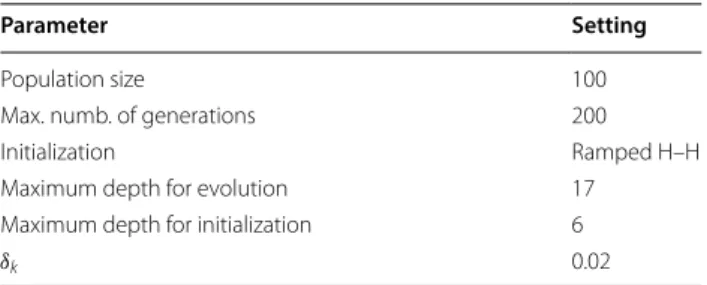
For each of the studied computational methods, 30 inde-pendent executions (runs) were performed, using a dif-ferent partitioning of the dataset into training and test set. More particularly, for each run 70% of the observa-tions were selected at random with uniform distribution to form the training set, while the remaining 30% form the test set. The parameters used are summarized in Table 2. Besides those parameters, the primitive opera-tors were addition, subtraction, multiplication, and divi-sion protected as in Koza (1992). The terminal symbols included one variable for each feature in the dataset, plus the following numerical constants: − 1.0, − 0.75, − 0.5, − 0.25, 0.25, 0.5, 0.75, 1.0. Parent selection was done using tournaments of size 5 for GSGP, and tournaments of size 10 for each layer of the nested selection for NAGP. The same selection as in NAGP was also performed in the first 50 generations of NAGP_50. Crossover rate was equal to zero (i.e., no crossover was performed during the evolution) for all the studied methods. While NAGP and NAGP_50 do not have a crossover operator implemented Table 1 The variables used to describe each instance in the studied dataset.

For each variable minimum, maximum, a kg/m3 _{average, median and standard deviation values are reported.}

ID Name (unit measure) Minimum Maximum Average Median Standard deviation

X0 Cement (kg/m3_{) 102.0 540.0 281.2 272.9 104.5}

X1 Fly ash (kg/m3_{) 0.0 359.4 73.9 22.0 86.3}

X2 Blast furnace slag (kg/m3_{) 0.0 200.1 54.2 0.0 64.0}

X3 Water (kg/m3_{) 121.8 247.0 181.6 185.0 21.4}

X4 Superplasticizer (kg/m3_{) 0.0 32.2 6.2 6.4 6.0}

X5 Coarse aggregate (kg/m3_{) 801.0 1145.0 972.9 968.0 77.8}

X6 Fine aggregate (kg/m3_{) 594.0 992.6 773.6 779.5 80.2}

X7 Age of testing (days) 1.0 365.0 45.7 28.0 63.2

Table 2 GP parameters used in our experiments.

Parameter Setting

Population size 100

Max. numb. of generations 200

Initialization Ramped H–H

Maximum depth for evolution 17

Maximum depth for initialization 6

yet, the motivation for not using crossover in GSGP can be found in Castelli et al. (2014).

6.3 Experimental Results, Comparison with GSGP The experimental results are organized as follows:

• Fig. 7 reports the results of the training error and the error of the best individual on the training set, evalu-ated on the test set (from now on, the terms training error and test error will be used for simplicity); • Fig. 8 reports the results of the size of the evolved

solutions (expressed as number of tree nodes); • Table 3 reports the results of the study of statistical

significance that we have performed on the results of the training and test error.

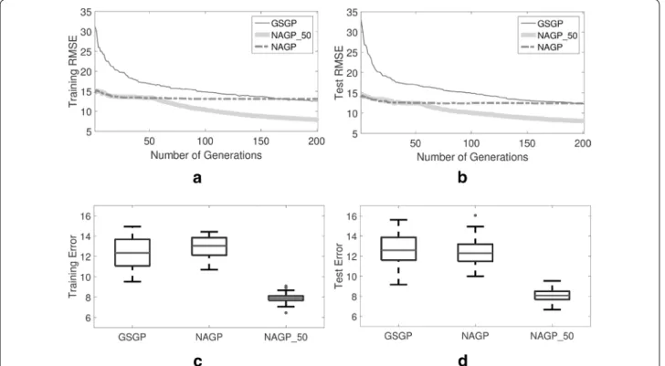
From Fig. 7, we can see that NAGP_50 clearly out-performs the other two studied methods both on training and on unseen data. Also, if we compare NAGP to GSGP, we can observe that these two meth-ods returned similar results, with a slight preference of GSGP on training data, and a slight preference of NAGP on unseen data. From plots of Fig. 7a, b, we can also have a visual rendering of how useful it is for NAGP_50 to “switch” from the NAGP algorithm to the GSGP algorithm after 50 generations. In fact, both on

the training and on the test set, it is possible to notice a rapid improvement of the curve of NAGP_50, which looks like a sudden descending “step”, at generation 50.

Now, let us discuss Fig. 8, that reports the dimensions of the evolved programs. GSGP and NAGP_50 gener-ate much larger individuals compared to NAGP. This was expected, given that generating large individuals is a known drawback of GSOs (Moraglio et  al. 2012). The fact that in the first 50 generations NAGP_50 does not use GSOs only partially limits the problem, simply delaying the code growth, that is, after generation 50, as strong as for GSGP. On the other hand, it is clearly vis-ible that NAGP is able to generate individuals that are

Fig. 7 Results of the error for the three studied methods. a Evolution of training error; b evolution of test error; c boxplots of the training error at

the end of the run; d boxplots of the test error at the end of the run. All results are medians over 30 independent runs.

much smaller: after a first initial phase in which also for NAGP the size of the individuals grows, we can see that NAGP basically has no further code growth (the curve, after an initial phase of growth, rapidly stabilizes and it is practically parallel to the horizontal axis). Last but not least, it is also interesting to remark that the final model generated by NAGP has around only 50 tree nodes, which is a remarkably small model size for such a complex application as the one studied here.

To analyse the statistical significance of the results of the training and test errors, a set of tests has been performed. The Lilliefors test has shown that the data are not normally distributed and hence a rank-based statistic has been used. The Mann–Whitney U-test for pairwise data comparison with Bonferroni correction has been used, under the alternative hypothesis that the samples do not have equal medians at the end of the run, with a significance level α = 0.05. The p-values are reported in Table 3, where statistically significant dif-ferences are highlighted with p-values in italics.

As we can observe, all the differences between the results obtained with all the studied methods are statis-tically significant.

The conclusion is straightforward: NAGP_50 out-performs GSGP in terms of prediction accuracy, but returns results that are comparable to the ones of GSGP in terms of the size of the model. On the other hand, NAGP outperforms GSGP in terms of prediction accu-racy on unseen data and also in terms of model size. 6.4 Experimental Results, Comparison Other Machine

Learning Techniques

This section compares the results obtained by NAGP and NAGP_50 with the ones achieved with other state-of-the-art machine learning (ML) methods. The same 30 different partitions of the dataset used in the previous part of the experimental study were considered. To run the ML techniques, we used the implementation pro-vided by the Weka public domain software (Weka 2018). The techniques taken into account are: linear regres-sion (LIN) (Weisberg 2005), isotonic regression (ISO) (Hoffmann 2009), an instance-based learner that uses an

entropic distance measure (K*) (Cleary and Trigg 1995), multilayer perceptron (MLP) (Haykin 1999) trained with back propagation algorithm, radial basis function net-work (RBF) (Haykin 1999), and support vector machines (SVMs) (Schölkopf and Smola 2002) with a polynomial kernel.

As done for the previous experimental phase, a pre-liminary study has been performed in order to find the best tuning of the parameters for all the considered techniques. In particular, using the facilities provided by Weka, we performed a grid search parameter tuning, where different combinations of the parameters were tested. Table 4 shows the interval of tested values for each parameter and for each technique.

The results of the comparison we performed are reported in Figs. 9 and 10 where the performance on the training and test sets are presented, respectively. We start the analysis of the results by commenting the perfor-mance on the training set.

As one can show in Fig. 9, K* is the best performer on the training set, producing better quality models with respect to all the other studied techniques. MLP is the second-best technique, followed by NAGP_50 and SVMs. LIN outperforms both GSGP and NAGP, while ISO pro-duces similar results with respect to NAGP. Finally, the worst performer is RBF. Focusing on NAGP_50, it is important to highlight that its performance is compara-ble to MLP and SVM, two techniques that are commonly used to address this kind of problem.

While the results on the training data are important, the performance on the test set is a fundamental indica-tor to assess the robustness of the model with respect to its ability to generalize over unseen instances. This is a property that must be ensured in order to use a ML tech-nique for addressing a real-world problem. According to Fig. 10, NAGP_50 outperforms all the other techniques taken into consideration on the test set. Interestingly, its performance is comparable with the one achieved on the training set, presenting no evidence of overfitting. This indicates that NAGP_50 produces robust models that are able to generalize over unseen data.

To assess the statistical significance of the results pre-sented in Figs. 9 and 10, the same type of statistical test as the ones presented in the previous section was per-formed, with α = 0.05 and the Bonferroni correction. Table 5 reports the p-values returned by the Mann– Whitney test with respect to the results achieved on the training set. Results reported in italic are those in which the null hypotheses can be rejected (i.e. the statistically significant results). According to these results, NAGP_50 produces results that are comparable with SVMs, while K* is the best performer followed by MLP.

Table 3 p-values returned by  the  Mann–Whitney U-test on  training and  test sets under  the  null hypothesis that the samples have the same median.

Italics denotes statistically significant values.

Training set Test set

NAGP NAGP_50 NAGP NAGP_50

GSGP 3.38E−08 3.58E−06 6.98E−06 2.18E−05

Table 6 reports the p-values of the Mann–Whitney test with respect to the results achieved on the test set. According to these p-values, it is possible to state the NAGP_50 is the best performer, producing solutions that outperform the other techniques in a statistically significant way. SVMs are not able to produce the same good-quality performance on the test set, overfitting the training data. Interestingly, all the non-GP techniques, except LIN, suffer from overfitting, hence producing models that are not able to generalize well on unseen data.

6.5 Experimental Results, Discussion of an Evolved Model In this section, we show and discuss the best multi-individual evolved by NAGP in our simulations. It is important to point out that, as Fig. 8 clearly shows, this would not be possible for NAGP_50 and for GSGP, since

these two methods use GSOs and these operators cause a rapid growth in the size of the evolved solutions. For this reason, it was not possible to show the final model in Cheng et al. (2013), while it is possible in the present contribution.

The best multi-individual evolved by NAGP in all the runs that we have performed was composed by the fol-lowing expressions, in prefix notation:

6.5.1 Expression 1 (* (* (* (* (* (* (* (* (* (* (* (* (* (* (* (* (* (* (* (* (* (* (* (* (* (* (* (* (* (* (* (* (* (* (* (* (* (* (* (* (* (* (* (* (* (* (* (* (* (* (* (* (* (* (* (* (* (* (* (* (* (* (* (* (* (* (* (* (* (* (* (* (* (* (* (* (* (* (* (* (* (* (* (* (* (* (* (* (* (* (* (* (* (+ (* X0 (− X6 (* (+ (− (/ (* X3 (− − 0.75 X5)) (/ (/ 0.5 (+ − 1.0 − 0.25)) (/− 1.0 0.75))) (− X1 (− (/ X7 0.25) (+ (* (/− 0.75 (+ X7 X0)) (* (− 1.0 X6) (− (* (/ (+ X2 X1) − 0.25) (+ (/ X7 Table 4 Parameter tuning.

For each technique, the table reports the tuned parameters and the value used in the experiments that were performed. The reader is referred to the Weka ML tool documentation (Weka 2018) for the explanation of these parameters.

Technique Parameter name Values tested [min;max;# of values tested] Best value

LIN ridge [1.0E−7;1.0E−9;3] 1.00E−08

eliminateColinearAttributes True; False True

ISO – – – K* globalBlend [0;100;10] 30 MLP learningRate [0.1;0.4;4] 0.15 momentum [0.1;0.4;4] 0.1 hiddenLayers [1, 7] 3 trainingTime [500;1000;5] 1000 RBF minStdDev [0.1;0.5;5] 0.2

ridge [1.0E−7;1.0E−9;3] 1.00E−08

SVM DegreePolynomialKernel [1, 4] 2

regOptimizer RegSMO; RegSMOimproved RegSMOimproved

Fig. 10 Root mean squared error on the test set.

Table 5 p-values returned by the Mann–Whitney U-test for the results achieved on the training set.

Italic is used to denote statistically significant differences between the considered techniques.

Training

GSGP NAGP NAGP50 LIN ISO K* MLP RBF SVM

GSGP – 2.19E−01 6.51E−11 1.39E−02 4.63E−02 6.26E−11 3.59E−08 6.26E−11 6.95E−11

NAGP – 6.51E−11 4.22E−07 4.01E−01 6.26E−11 1.22E−08 6.26E−11 6.26E−11

NAGP50 – 6.26E−11 6.26E−11 6.26E−11 1.16E−01 6.26E−11 3.56E−02

LIN – 1.87E−10 6.03E−11 2.13E−07 6.03E−11 6.03E−11

ISO – 6.03E−11 1.56E−08 6.03E−11 6.03E−11

K* – 6.03E−11 6.03E−11 6.03E−11

MLP – 6.03E−11 2.80E−03

RBF – 6.03E−11

SVM –

Table 6 p-values returned by the Mann–Whitney U-test for the results achieved on the test set.

Italic is used to denote statistically significant differences between the considered techniques.

Test

GSGP NAGP NAGP50 LIN ISO K* MLP RBF SVM

GSGP – 4.19E−01 1.45E−09 3.31E−07 5.11E−08 5.86E−01 6.41E−01 1.16E−09 1.87E−04

NAGP – 1.20E−09 7.25E−08 1.88E−09 6.52E−01 4.27E−01 6.26E−11 2.25E−04

NAGP50 – 1.71E−09 1.16E−09 1.16E−09 1.16E−09 1.16E−09 2.07E−09

LIN – 6.07E−11 6.06E−11 2.98E−07 6.06E−11 4.79E−05

ISO – 4.28E−09 1.60E−03 1.12E−09 6.04E−11

K* – 9.88E−01 6.03E−11 2.96E−06

MLP – 9.83E−05 3.55E−02

RBF – 6.03E−11

(+ − 0.5 (/ (/ X4 (+ − 1.0 X1)) X7))) (− (− 0.25 1.0) (+ (+ X7 X1) (− 1.0 − 0.25))))) 0.5))) 0.5)))) (− (/ (− (+ − 0.5 (*− 0.25 0.75)) (/ (* (/ X5 (− − 0.25 0.5)) (+ X0 (− (/ (− − 0.25 X3) (/ (/ (/ (/ (− (* (/ X2− 1.0) X0) X6)− 0.25) (/ (/ (+ − 0.25− 1.0) (+ X7− 0.5)) (+ − 0.25 − 0.75))) X1) X1)) − 0.75))) (/ (/ (/ (+ X6 (/ 0.25 (*− 0.75 1.0))) 0.75) (+ − 1.0 (+ 1.0 X3)))− 1.0))) (/ X6 (/ (+ (+ X6 − 1.0) (*− 0.5 (− 1.0 (− − 0.75 X3)))) 0.75)))− 0.25)) (/ X7 (* (+ − 0.75 (/ 1.0 (* (/ X6 (/ 0.75 (+ 0.75 X4))) (* (− (+ − 0.25 X4) 0.75) (* X6 (/ (* (/− 0.25 (+ (− − 0.5 X6) 1.0)) (− X6 0.25)) X7)))))) X7))))) (* X7 − 0.5)) 34.0) X5) 33.0) 36.0) X6) 23.0) 31.0) 23.0) 20.0) 31.0) 39.0) 39.0) (− X6 1.0)) 36.0) 28.0) 34.0) 22.0) 25.0) 38.0) 26.0) 29.0) 34.0) 27.0) 30.0) 23.0) 33.0) 35.0) 24.0) 34.0) 36.0) 36.0) 37.0) 38.0) 36.0) 27.0) 39.0) 36.0) 20.0) 34.0) 37.0) 37.0) 37.0) 36.0) 32.0) 37.0) 39.0) 33.0) 26.0) 39.0) 31.0) 33.0) 24.0) 27.0) 27.0) 33.0) 39.0) 37.0) 38.0) 36.0) 32.0) 23.0) 35.0) 24.0) 39.0) 26.0) 26.0) (+ (+ X0 (* (− 1.0 (+ (/ X2 0.75) − 0.75))− 0.5)) (+ (* X1 1.0) X7))) 26.0) 37.0) 37.0) 27.0) 32.0) 38.0) 22.0) 37.0) 34.0) 31.0) 28.0) 30.0) 21.0) 26.0) 23.0) 20.0) 38.0) 38.0) 33.0) 32.0) 21.0) 24.0) 20.0) 37.0) 30.0) 21.0). 6.5.2 Expression 2 (* (* (/X4 (+ X7 (+ (* (− (− (/(* (− (/(+ 1.0 X3) (− X1 (− (− X2 X6) − 0.75))) (− (/(− X2 X4) (* (+ (/(+ − 1.0 0.25) (+ 0.25 X0)) (+ X3 (− X3 0.5))) X4)) X4)) X1) (/0.75− 0.25)) (− X5 − 1.0)) (+ − 0.5 0.5)) (/− 1.0 X2)) (− X6 X2)))) X7) 21.0).

The reader is referred to Table 1 for a reference to the different variables used in this expression (only the IDs—X0, X1,…, X7—referenced in the table are used in the above expressions). If we consider the reconstructed expression Popt [as in Eq. (3)] using these two expressions, Popt has an error on the training set equal to 9.53 and

an error on the test set equal to 9.06. Both the relation-ship between the training and test error (they have the same order of magnitude and the error on the test set is even smaller) and a comparison with the median results reported in Fig. 7 allow us to conclude that this solution has a very good performance, with no overfitting.

The first thought that comes to mind when watch-ing these two expressions is that the first one is signifi-cantly different from the second one: first of all in terms of size (the first expression is clearly larger than the sec-ond), but also in terms of tree shape. Observing the first expression, in fact, one may notice a sort of skewed and

unbalanced shape consisting of several multiplications by constant numbers. This observation is not surprising: the first of these two expressions, in fact, is the one that has undergone the multiplication by the constant λ dur-ing the mutation events, as explained in Sect. 5. These continuous multiplications by constants have, of course, also an impact on the size of the expression (this is the reason why the first expression is larger than the sec-ond one). However, it is easy to understand that all these multiplications by a constant can be easily simplified, i.e. transformed into one single multiplication by a constant. Concerning the second expression, instead, we can see that it is much simpler and quite easy to read (numeric simplifications are possible also on this second expres-sion, which would make it even simpler and easier to read).

Concerning the variables used by the two models, Table 7 shows the number of times that each of the varia-bles appears in these two expressions. From this table, we can see that variables X6 and X7 are the ones that appear most frequently in the expressions, and thus we hypoth-esize that these variables are considered as the most useful, i.e. informative, ones by NAGP for the correct reconstruction of the target. These variables represent fine aggregate (expressed in kg/m3_{) and age of testing}

(expressed in number of days), respectively.

7 Conclusions and Future Work

High-performance concrete is one of the most com-monly used human-made artifacts nowadays. It is a very complex material and optimizing it in order to obtain the desired behavior is an extremely hard task. For this reason, effective computational intelligence systems are much in demand. In particular, the task of predict-ing the strength of high-performance concrete is very difficult and the problem has been the focus of a recent investigation. This paper extends a recent publication of our research group (Castelli et al. 2013), significantly improving the results. In that paper, we proposed a new Genetic Programming (GP) system, called Geometric Semantic GP (GSGP), for the prediction of the strength of high-performance concrete, showing that GSGP was able to outperform existing methods. In this work, we propose a new system, called Nested Align GP (NAGP), with the objective of further improving the results that we obtained with GSGP. As for GSGP, NAGP integrates semantic awareness in the evolutionary process of GP. Table 7 Number of occurrences of each variable in the expressions presented in Sect. 6.5.

Variable X0 X1 X2 X3 X4 X5 X6 X7

However, differently from GSGP, NAGP exploits a new and promising concept bound to semantics, i.e. the con-cept of alignment in the error space. In order to effec-tively take advantage of the concept of alignment, NAGP evolves set of expressions (instead of single expressions, like traditional GP or GSGP do), that we have called multi-individuals. Furthermore, a variant of NAGP, called NAGP_β was presented, that is able to switch, at a prefixed generation β, from a multi-individual tation to a more traditional single-expression represen-tation. The presented experiments show that the results returned by NAGP and NAGP_ β improve the ones of GSGP from two different viewpoints: on one hand, both NAGP and NAGP_ β significantly outperform GSGP from the point of view of the prediction accuracy; sec-ondly, NAGP is able to generate predictive models that are much smaller, and thus more readable and interpret-able, than the ones generated by GSGP. In this way, in this paper we have been able to show a model evolved by NAGP, which was impossible in Castelli et al. (2013). These results allow us to foster NAGP as the new state-of-the-art for high-performance concrete prediction with computational intelligence.

Future work can be divided into two main parts: the work that is needed, and planned, to further improve NAGP and its variant, and the work that we intend to perform to further improve the results on the prediction of the strength of high-performance concrete.

Concerning NAGP, we believe that one of the most important limitations of this paper is that only align-ments in two dimensions are considered. In other words, NAGP evolves individuals that are pairs of programs and so NAGP is only able to search for pairs of opti-mally aligned programs. Our current research is focused on extending the method to more than two dimensions. For instance, we are currently working on the develop-ment of systems that evolve individuals that are triplets of programs, aimed at finding triplets of optimally copla-nar individuals. The subsequent step will be to further extend the method, possibly generalizing to any number of dimensions. The design of self-configuring methods, that automatically decide the most appropriate dimen-sion, is one of the most ambitious goals of our current work. Concerning NAGP_β, a methodological study on the impact of the β parameter is planned. Last but not least, we are planning to study and develop several differ-ent possible types of crossover for NAGP.

Concerning possible ways of improving the prediction of the strength of high-performance concrete, we are cur-rently working on two different, although related, direc-tions: on one hand, we are developing a new algorithm that integrates clustering techniques as a pre-processing step. On the other hand, we are also planning to develop

a system that is highly specialized for high-performance concrete strength prediction, integrating into the system a set of rules coding some problem knowledge coming from domain experts. Last but not least, we are plan-ning to validate the proposed systems on other real-life datasets.

Authors’ contributions

LV and MC designed the proposed method. KS implemented the system and performed the experiments. AP performed the statistical analysis and proof-read the paper. All the authors wrote the paper. All authors proof-read and approved the final manuscript.

Author details

1 _{NOVA Information Management School (NOVA IMS), Universidade Nova de}

Lisboa, Campus de Campolide, 1070-312 Lisbon, Portugal. 2 _{Faculty of}

Eco-nomics, University of Ljubljana, 1000 Ljubljana, Slovenia. Competing interests

The authors declare that they have no competing interests.

Publisher’s Note

Springer Nature remains neutral with regard to jurisdictional claims in pub-lished maps and institutional affiliations.

Received: 27 November 2017 Accepted: 24 July 2018

References

Abrams, D. A. (1927). Water-cement ration as a basis of concrete quality. ACI Materials Journal, 23(2), 452–457.

Bhanja, S., & Sengupta, B. (2005). Influence of silica fume on the tensile strength of concrete. Cement and Concrete Research, 35(4), 743–747. Castelli, M., Silva, S., & Vanneschi, L. (2015). A C ++ framework for geometric

semantic genetic programming. Genetic Programming and Evolvable Machines, 16(1), 73–81.

Castelli, M., Vanneschi, L., & Silva, S. (2013). Prediction of high performance concrete strength using genetic programming with geometric semantic genetic operators. Expert Systems with Applications, 40(17), 6856–6862. Castelli, M., Vanneschi, L., Silva, S., & Ruberto, S. (2014). How to exploit

align-ment in the error space: Two different gp models. In R. Riolo, W.P. Worzel, & M. Kotanchek (Eds.), Genetic programming theory and practice XII, genetic and evolutionary computation (pp. 133–148). Ann Arbor, USA: Springer. Cheng, M. Y., Firdausi, P. M., & Prayogo, D. (2014). High-performance concrete

compressive strength prediction using Genetic Weighted Pyramid Operation Tree (GWPOT). Engineering Applications of Artificial Intelligence, 29, 104–113.

Cheng, M. Y., Prayogo, D., & Wu, Y. W. (2013). Novel genetic algorithm-based evolutionary support vector machine for optimizing high-performance concrete mixture. Journal of Computing in Civil Engineering, 28(4), 06014003.

Chou, J. S., Chiu, C. K., Farfoura, M., & Al-Taharwa, I. (2010). Optimizing the prediction accuracy of concrete compressive strength based on a comparison of data-mining techniques. Journal of Computing in Civil Engineering, 25(3), 242–253.

Cleary, J. G., & Trigg, L. E. (1995). K*: An instance-based learner using an entropic distance measure. In Machine learning proceedings 1995 (pp. 108–114).

Eiben, E., & Smith, J., E. (2003). Introduction to evolutionary computing. Berlin: Springer.

Frank, E, Hall, M. A., & Witten, I. H. (2016). The WEKA workbench. Online Appen-dix for “Data Mining: Practical Machine Learning Tools and Techniques” (4th ed.). Morgan Kaufmann.

Gonçalves, I., Silva, S., Fonseca, C. M., & Castelli, M. (2016). Arbitrarily close alignments in the error space: A geometric semantic genetic program-ming approach. In Proceedings of the 2016 on Genetic and Evolutionary