(Annals of the Brazilian Academy of Sciences)
Printed version ISSN 0001-3765 / Online version ISSN 1678-2690 www.scielo.br/aabc
http://dx.doi.org/10.1590/0001-3765201520140299
AMS (2010): 60E05, 62E10, 62N05 Correspondence to: Saralees Nadarajah E-mail: [email protected]
Parameter induction in continuous univariate
distributions: Well-established
G
families
MUHAMMAD H. TAHIR1 and SARALEES NADARAJAH2
1
Department of Statistics, Baghdad Campus, The Islamia University of Bahawalpur, Bahawalpur 63100, Pakistan 2School of Mathematics, University of Manchester, Oxford Road, Manchester, M13 9PL, UK
Manuscript received on June 9, 2014; accepted for publication on November 25, 2014
ABSTRACT
The art of parameter(s) induction to the baseline distribution has received a great deal of attention in recent years. The induction of one or more additional shape parameter(s) to the baseline distribution makes
the distribution more flexible especially for studying the tail properties. This parameter(s) induction also proved helpful in improving the goodness-of-fit of the proposed generalized family of distributions. There exist many generalized (or generated) G families of continuous univariate distributions since 1985. In this paper, the well-established and widely-accepted G families of distributions like the exponentiated family,
Marshall-Olkin extended family, beta-generated family, McDonald-generalized family, Kumaraswamy-generalized family and exponentiated Kumaraswamy-generalized family are discussed. We provide lists of contributed
literature on these well-established G families of distributions. Some extended forms of the Marshall-Olkin
extended family and Kumaraswamy-generalized family of distributions are proposed.
Key words: Beta-distribution, exponentiated family, Kumaraswamy distribution, Marshall-Olkin family, McDonald distribution, reliability properties.
INTRODUCTION
There has been an increased interest in developing generalized (or generated)
G
families of distributions
by introducing one or more additional shape parameter(s) to the base- line distribution. There is no doubt
that the popularity and the use of Euler-beta and -gamma functions in some
G
families of distributions have
attracted the attention of statis- ticians, mathematicians, scientists, engineers, economists, demographers
and other applied researchers. One reason might be the computational and analytical facilities available
in programming softwares like R (packages), ox5, Python, Matlab, Maple and Mathematica, through
which researchers can easily tackle problems involved in computing incomplete- beta and -gamma
functions in
G
families. The second reason is the tail properties of
G
distributions that can easily be
explored by inducting one or more additional shape param- eter(s) to the baseline distribution. Thirdly,
this parameter(s) induction has also proved to be helpful in improving the goodness-of-fit of the proposed
distributions (Pescim et al. 2010). Lastly, the Kumaraswamy
G
family of distributions can generate
effective models for censored data (Cordeiro and de Castro 2011).
There exists many generalized (or generated)
G
family of distributions like Azzalini’s skewed family
(Azzalini 1985), Marshall-Olkin extended (MOE) family (Marshall and Olkin 1997), exponentiated family
(EF) of distributions (Gupta et al. 1998), beta-generated (beta
G
) family (Eugene et al. 2002, Jones 2004a),
Ferreira and Steel’s skewed family (Ferreira and Steel 2006), transmutated family (Shaw and Buckley 2007,
Aryal and Tsokos 2009, 2011), Gupta and Gupta’s skewed family (Gupta and Gupta 2008), gamma-generated
(GG) families (Zografos and Balakrishnan 2009, Ristić and Balakrishnan 2012, Torabi and Montazari 2012,
Nadarajah et al. 2015), transformed-transformer (T-X) family (Alza-Atreh 2011), Kumaraswamy generalized
(Kw
G
) family (Cordeiro and de Castro 2011, Nadarajah et al. 2012a, Hussain 2013), generalized beta
generated (GBG) or McDonald generalized (Mc
G
) family (Alexander et al. 2012), beta extended
G
family
(Cordeiro et al. 2012f), Kummer beta generalized family (Pescim et al. 2012), exponentiated transformed-
transformer family (ET-X) (Alzaghal et al. 2013), exponentiated generalized (Exp
G
) family (Cordeiro et
al. 2013e), geometric exponential-Poisson family (Nadarajah et al. 2013a), truncated-exponential
skew-symmetric family (Nadarajah et al. 2013c), logistic-generated (Lo
G
) family (Torabi and Montazari 2014),
Marshall-Olkin extended family (Alshangiti et al. 2014), log-gamma generated (LG
G
) families, (Amini et
al. 2014), Weibull
G
family (Bourguignion et al. 2014), Libby-Novick beta family (Cordeiro et al. 2014e),
truncated negative-binomial family (Nadarajah et al. 2014a), modified beta
G
family (Nadarajah et al. 2014b)
and exponentiated exponential-Poisson family (Ristić and Nadarajah 2014). These
G
families of distributions
have received a great deal of attention in recent years. In this paper, we discuss the EF, MOE, beta
G
, Mc
G
,
Exp
G
and Kw
G
families of distri- butions and provide additional literature (in chronological order) on these
six families of distributions. We also propose some extended forms of the Kw
G
families of distributions by
introducing one more additional shape parameter(s).
Because of the length of this paper, we have not given details like probabilistic interpretations,
analytical properties, estimation methods, simulation algorithms and applications. These details can be
obtained from the cited references.
The rest of the paper is organized as follows. In Section 2, the EF of distributions is defined and a list
of contributed work is presented. In Section 3, we describe the MOE family and propose one generalized
MOE family of distributions. The contributed literature on the MOE family is also presented. In Section 4,
the beta
G
family of distributions is discussed. The contributions to the beta
G
family of distributions are
also listed in this section. In Section 5, the McDonald distributions and Mc
G
families of distributions are
described. The contributed work on Mc
G
families of distributions is also presented. Section 6 consists of
Kumaraswamy distributions and Kw
G
families of distributions. Some new types of the Kumaraswamy
distribution and Kw
G
families of distributions are proposed. The contributed work on the Kw
G
family of
distributions is also listed in this section. Section 7 ends the paper with some final remarks.
EXPONENTIATED FAMILY (EF) OF DISTRIBUTIONS
The genesis of this family can be traced back to the first half of the nineteenth century when Gompertz (1825)
and Verhulst (1838, 1845, 1847) used the cumulative distribution function (cdf)
G
(
t
) = (1
−
ρ e
−λt)
αfor
t >
for
ρ
= 1. The properties and estimation methods for parameters of the EF of distributions have been studied
by many authors, see Mudholkar and Srivastava (1993), Mudholkar and Hutson (1996), Mudholkar et al.
(1995), Gupta and Kundu (1999, 2001a, b, 2007), Pal et al. (2006), Nadarajah and Kotz (2006a), Nadarajah
(2011) and Nadarajah et al. (2013b). The EF of distributions is also known as Lehmann alternatives (LAs)
(Lehmann 1953) or proportional reversed hazard rate model (PHRM) (see Gupta et al. 1998, Gupta and Gupta
2007, Martínez-Florez et al. 2013), while other authors referred to the EF of distributions as max-stable family
(Sarabia and Castillo 2005) and
F
α- distributions (Gupta et al. 1998, Al-Hussaini, 2010a, b, 2012, Shakil
and Ahsanullah 2012, Hamedani 2013 and Ghitany et al. 2013).
In literature there exist four different ways for obtaining the EF of distributions.
LEHMANN ALTERNATIVE 1(LA1)
The method of Lehmann alternative 1 (LA1) (due to Lehmann (1953)) has received a great deal of attention
in developing the EF of distributions.
If
G
(
z
) is the cdf of the baseline distribution, then an EF of distributions is defined by taking the
α
th-power of
G
(
z
) as
F
(
z
) =
G
(
z
)
α,
(2.1)
where
α >
0 is a positive real parameter. The variable
z
can take any of the form
z
=
x
or
z
=
x −
µ
or
z
=
x‒µσor
z
=
k
³x‒µσ ´or
z
=
k
³x‒µσ ´1
δ
. The probability density function (pdf) corresponding to (2.1) is
f
(
z
) =
αg
(
z
)
G
(
z
)
α‒1,
(2.2)
where
g
(
z
) =
dG
(
z
)
/dz
denotes the pdf of
G
. For any lifetime random variable
t
, the survival (reliability)
function (sf),
F
(
t
), the hazard (failure) rate function (hrf),
h
(
t
), the reversed hazard rate function (rhrf),
r
(
t
),
and the cumulative hazard rate function (chrf),
H
(
t
), associated with (2.1) and (2.2) are
F
(
t
) = 1 −
G
(
t
)
α,
h
(
t
) =
αg
(
t
)
G
(
t
)
α−1[1 −
G
(
t
)
α]
−1,
r
(
t
) =
αg
(
t
)
G
(
t
)
−1,
and
H
(
t
) = −log [1 −
G
(
t
)
α].
LEHMANN ALTERNATIVE 2(LA2)
The method of Lehmann alternative 2 (LA2) (due to Lehmann (1953)) has received less attention.
If
G
(
z
) is the cdf and
G
(
z
) = 1
−
G
(
z
) is the sf of the baseline distribution, then an EF of distributions
is defined by taking one minus the
α
th-power of
G
(
z
) as
F
(
z
) = 1
−
[
G
(
z
)]
α,
where
α
is a positive real parameter. The LA2 cdf may also be written as
F
(
z
) = 1
−
[1
−
G
(
z
)]
α.
(2.3)
The pdf corresponding to (2.3) is
For any lifetime random variable
t
, the sf, hrf, rhrf and chrf associated with (2.3) and (2.4) are
F
(
t
) = [1
−
G
(
t
)]
α,
h
(
t
) =
αg
(
t
) [1
−
G
(
t
)]
−1,
r
(
t
) =
αg
(
t
) [1
−
G
(
t
)]
α−1{1
−
[1
−
G
(
t
)]
α}
−1,
and
H
(
t
) =
−α
log [1
−
G
(
t
)].
Nadarajah and Kotz (2003, 2006a), Nadarajah (2006) and Rao et al. (2013) used the LA2 approach for
introducing exponentiated Fréchet, exponentiated Gumbel and exponen- tiated log-logistic distributions.
For more applications of the LA2 approach, the reader is referred to Elfattah and Omima (2009),
Abd-Elfattah et al. (2010), Rao et al. (2012, 2013), and Al-Nasser and Al-Omari (2013).
USING TRANSFORMATION z = log(x), x > 0
Nadarajah (2005a) developed exponentiated distributions by applying the transformation
z
= log(
x
) to (2.3).
The cdf, pdf and the hrf of the exponentiated distribution are
F
(
x
) = 1
−
[1
− G
(
e
x)]
α,
f
(
x
) =
ae
xg
(
e
x) [1
− G
(
e
x)]
α−1and
h
(
x
) =
ae
xg
(
e
x) [1
−
G
(
e
x)]
−1.
USING TRANSFORMATIONz = − log(x), x > 0
Nadarajah (2005b) developed exponentiated distributions by applying the transformation
z
=
−
log(
x
) to (2.3).
The cdf, pdf and the hrf of the exponentiated distribution are
F
(
x
) = [1
− G
(
e
−x)]
α,
f
(
x
) =
ae
−xg
(
e
−x) [1
− G
(
e
−x)]
α−1and
h
(
x
) =
ae
−xg
(
e
−x) [1
−
G
(
e
−x)]
α−1{1
−
[1
−
G
(
e
−x)]
α}
−1.
A list of papers on the EF of distributions is presented in Table I.
S.No. Pioneer year Distribution Author(s)
1 1967 Exponentiated exponential distribution Ahuja and Nash (1967) Gupta et al. (1998)
Gupta and Kundu (1999, 2001a, b, 2007) Nadarajah (2011)
Venkatesan and Sundaram (2011) 2 1993 Exponential Weibull distribution Mudholkar and Srivastava (1993)
Mudholkar et al. (1995) Mudholkar and Hutson (1996) Gupta et al. (1998)
Jiang and Murthy (1999)
TABLE I
TABLE I (continuation)
S.No. Pioneer year Distribution Author(s)
Nassar and Eissa (2003) Choudhury (2005)
Nadarajah and Gupta (2005) Singh et al. (2005)
Pal et al. (2006) Ahmed et al. (2008)
Saleem and Abo-Kasem (2011)
Mazucheli et al. (2012)
Qian (2012)
Barrios and Dios (2012) Nadarajah et al. (2013b) 3 1998 Exponentiated gamma distribution Gupta et al. (1998)
Nadarajah and Kotz (2006a)
Nadarajah and Gupta (2007)
Shawky and Bakoban (2008, 2009, 2012) 4 1998 Exponentiated Pareto distribution Gupta et al. (1998)
Nadarajah (2005a)
Shawky and Abu-Zinadah (2009)
Afify (2010)
5 2001 Exponentiated Rayleigh distribution Surles and Padgett (1998, 2001, 2005) Raqab (1998)
Kundu and Raqab (2005) Raqab and Kundu (2006) Raqab and Madi (2009, 2011) Abd-Elfattah (2011)
6 2003 Exponentiated Fréchet distribution Nadarajah and Kotz (2003)
Nadarajah and Kotz (2006a)
Abd-Elfattah and Omima (2009) Abd-Elfattah et al. (2010) Jamjoom and Al-Saiary (2012) Al-Nasser and Al-Omari (2013) Marwa et al. (2013)
7 2004 Exponentiated generalized Pareto distribution Adeyemi and Adebanji (2004) 8 2005 Exponentiated beta distribution Nadarajah (2005b)
9 2006 Exponentiated generalized extreme value distribution Adeyemi and Adebanji (2006) 10 2006 Exponentiated log-logistic distribution Rosaiah et al. (2006)
Aslam and Jun (2010) Rao et al. (2012, 2013) 11 2006 Exponentiated Gumbel distribution Nadarajah (2006)
Nadarajah and Kotz (2006a)
Shirke and Kakade (2007) Kakade et al. (2008) Persson and Rydén (2010) 12 2006 Exponentiated log-normal distribution Shirke and Kakade (2006)
Raja and Mir (2011) 13 2008 Exponential modified Weibull distribution Carrasco et al. (2008)
TABLE I (continuation)
S.No. Pioneer year Distribution Author(s)
17 2011 Exponentiated Burr XII distribution Al-Hussaini and Hussein (2011a, b) Maswadah (2013)
18 2011 Exponentiated generalized gamma distribution Cordeiro et al. (2011a) 19 2011 Exponentiated generalized inverse Gaussian distribution Lemonte and Cordeiro (2011) 20 2012 Exponentiated inverted Weibull distribution Flaih et al. (2012)
Kim et al. (2012) Hassan (2013) Aljuaid (2013) 21 2012 Exponentiated Kumaraswamy distribution Kumar (2012)
22 2012 Exponentiated Lomax distribution Abdul-Moniem and Abdel-Hameed (2012) 23 2012 Exponentiated Gompertz distribution El-Gohary (2012)
24 2013 Exponentiated modified Weibull extension distribution Sarhan and Apaloo (2013) 25 2013 Exponentiated generalized linear exponential distribution Sarhan et al. (2013) 26 2013 Exponentiated Dagum distribution Khan (2013) 27 2013 Exponentiated sinh Cauchy distribution Cooray (2013)
28 2015 Exponentiated geometric distribution Chakraborty and Gupta (2015)
MARSHALL-OLKIN EXTENDED (MOE) FAMILY OF DISTRIBUTIONS
Marshall and Olkin (1997) proposed a flexible semi-parametric family of distributions and defined a new sf
F
MO(
x
) by introducing an additional parameter
α >
0. Marshall and Olkin (1997) called
α
a tilt parameter
and interpreted
α
in terms of the behavior of the hrfs of
F
MOand
G
. Their ratio is increasing in
t
for
α ≥
1 and decreasing in
t
for 0
< α <
1. Nanda and Das (2012) reinterpreted
α
as a tilt parameter since the
hrf of the new family is shifted below (
α ≥
1) or above (0
< α ≤
1) the hrf of the underlying distribution.
Specifically, for all
t ≥
0,
h
MO(t
)
≤
h
(
t
) when
α ≥
1, and
h
MO(
t
)
≥
h
(
t
) when 0
< α ≤
1, where
h
MO(t
) and
h
(
t
)
are the hrfs of the MOE and baseline distributions.
For any baseline pdf
g
(
t
), cdf
G
(
t
) =
P
(
T ≤
t
) and sf
G
(
t
) =
P
(
T > t
) of the baseline distribution, the sf
F
MO(
t
) of the MOE family of distributions is defined by
F
MO(
t
) =
aG
(
t
)
1
−
aG
(
t
)
=
aG
(
t
)
G
(
t
)
+ aG
(
t
)
or
a
[1
−
G
(
t
)]
a
+ aG
(
t
)
,
(3.1)
where
−∞
< t < ∞
,
α >
0 and
a
= 1
−
α
. The cdf and pdf associated with (3.1) are
F
MO(
t
) =
G
(
t
)
1
−
aG
(
t
)
=
G
(
t
)
G
(
t
)
+ aG
(
t
)
or
1
−
G
(
t
)
a
+ aG
(
t
)
,
and
f
MO(
t
) =
ag
(
t
)
[1 −
aG
(
t
)]
2or
ag
(
t
)
[
a
+
aG
(
t
)]
2,
where −∞ < t < ∞,
α
> 0 and
a
= 1 −
α
. If
α
= 1, then we have
F
MO(
t
) =
G
(
t
). Other reliability measures like
the hrf, rhrf and chrf associated with (3.1) are
h
MO(
t
) =
f
MO(
t
)
F
MO(
t
)
=
g
(
t
)
G
(
t
)
1
[1 −
aG
(
t
)]
=
h
(
t
)
1 −
aG
(
t
)
or
h
(
t
)
r
MO(
t
) =
f
MO(
t
)
F
MO(
t
)
=
a
g
(
t
)
G
(
t
)
1
[1 −
aG
(
t
)]
=
ah
(
t
)
1 −
aG
(
t
)
or
ah
(
t
)
a
+
aG
(
t
)
,
and
H
MO(
t
) =
−log
aG
(
t
)
1 −
aG
(
t
)
or
−log
(
a
[
1 −
G
(
t
)]
)
a
+
aG
(
t
)
,
where
h
(
t
) is the hrf of the baseline distribution.
Note that if w
e define
F
MO(
t
) =
G
(
t
)
1
−
aG
(
t
)
then
F
MO(
t
) =
1 −
aG
(
t
)
aG
(
t
)
and
f
MO
(
t
) =
g
(
t
)
[1 −
aG
(
t
)]
2,
For more general results on the MOE family of distributions, the reader is referred to Barakat et al.
(2009), Jose (2011), Krishna (2011), Barreto-Souza et al. (2013) and Cordeiro et al. (2014c).
EXISTING GENERALIZED MOEFAMILY OF DISTRIBUTIONS
In this section, we describe existing generalized Marshall-Olkin families of distributions.
Jayakumar and Mathew (2008) proposed a generalization of the Marshall and Olkin (1997) family
of distributions (by using the LA1 approach) as
F
GMO(
t
) =
aG
(
t
)
1
−
aG
(
t
)
θ,
(3.2)
where
−∞
< t < ∞
,
α >
0, and
θ >
0 is an additional shape parameter. When
θ
= 1,
F
GMO(
t
) =
F
MO(
t
).
The cdf and the pdf associated with (3.2) are
F
GMO(
t
) =
1 −
aG
(
t
)
1 −
aG
(
t
)
θ
,
and
f
GMO(
t
) =
θ
aG
(
t
)
1 −
aG
(
t
)
θ − 1
(
ag
(
t
)]
)
[1 −
aG
(
t
)]
2.
Other reliability measures like the hrf, rhrf and chrf associated with (3.2) are
h
GMO(
t
) =
θ
g
(
t
)
G
(
t
)
1
1 −
aG
(
t
)
=
θh
(
t
)
1
1 −
aG
(
t
)
, or
θh
(
t
)
a
+
aG
(
t
)
,
r
GMO(
t
) =
θ a
θg
(
t
)
G
(
t
)
θ −1[1 −
aG
(
t
)]
θ−
a
θG
(
t
)
θ,
and
H
GMO(
t
) =
−log
(
1 −
aG
(
t
)]
θ)
[1 −
aG
(
t
)]
,
ANEW GENERALIZED MOEFAMILY OF DISTRIBUTIONS
Here, we propose another generalization of the Marshall and Olkin (1997) family of distributions.
Using the LA2 approach to the sf of the MOE family of distributions, we obtain
F
G2MO(
t
) =
1 −
1 −
aG
(
t
)
θ
1 −
aG
(
t
)
,
(3.3)
where −∞ <
t
< ∞,
α
> 0, and
θ
> 0 is the additional shape parameter. When
θ
= 1,
F
G2MO(t) =
F
MO(t).
The cdf and the pdf associated with (3.3) are
F
G2MO(
t
) =
1 −
aG
(
t
)
θ1 −
aG
(
t
)
,
and
f
G2MO(
t
) =
θ
1 −
aG
(
t
)
θ − 11 −
aG
(
t
)
(
ag
(
x
)
)
[1 −
aG
(
t
)]
2.
After simplification, the above pdf can be rewritten as
f
G2MO(
t
) =
θ ag
(
t
)
G
(
t
)
θ −11 −
aG
(
t
)
or
θ ag
(
t
)
G
(
t
)
θ −1a
+
aG
(
t
)
.
Other reliability measures like the hrf, rhrf and chrf associated with (3.3) are
h
G2MO(
t
) =
θ ag
(
t
)
G
(
t
)
θ −1[
a
+
aG
(
t
)]
θ +1(
1 − 1 −
aG
(
t
)
θ)
−1[1 −
aG
(
t
)]
,
r
G2MO(
t
) =
θ a g
(
t
)
G
(
t
)
1
a
+
aG
(
t
)
=
θ a r
(
t
)
a
+
aG
(
t
)
,
and
H
G2MO(
t
) =
− log
(
1 − 1 −
aG
(
t
)
θ)
[1 −
aG
(
t
)]
,
where
r
(
t
) is the rhrf of the baseline distribution.
The construction in (3.3) is similar to that due to Jayakumar and Mathew (2008). But there is
an important distinction. Suppose that a system consists of
θ
independent components. Suppose too
that each component has a lifetime with the sf given by
α
G
(
t
)
/
[ 1
−
aG
(
t
)]. Then (3.2) is the sf of the
minimum of the lifetimes and (3.3) is the sf of the maximum of the lifetimes. So, (3.2) can be used
to model the minimum of the lifetimes and (3.3) can be used to model the maximum of the lifetimes.
SEMI-TYPE PROCESSES BASED ON CHARACTERISTIC FUNCTION
In this section, we briefly discuss semi-Pareto, semi-Burr, semi-Laplace, semi-logistic and semi-Weibull
distributions based on the characteristic function (cf)
ψ
(
t
) of the baseline distribution. The concept of
semi-type distributions arose from the minification process. Tavares (1980) defined a minification process as
observations in a process generated by
X
n=
k
min (
X
n−1,
²
n) ,
(3.4)
where
n ≥
1,
k >
1 is a constant and
{
²
n}
is an innovation process of independent and identically
distributed random variables. Here,
{X
n}
is called the first order autoregressive AR(1) minification process.
Linnik (1963) introduced the
α
-Laplace distribution, a symmetric distribution defined on (
−∞, ∞
). For
α
= 2,
the Linnik distribution reduces to the Laplace distribution. Pillai
(1985) generalized the Linnik distribution
and introduced the semi-
α
-Laplace distribution.
Yeh et al. (1988) modified (3.4) and introduced the first auto-regressive Pareto minification process
having Pareto marginals. Arnold and Robertson (1989) introduced minification processes with logistic
marginals. Pillai (1991) and Pillai et al. (1995) introduced semi-Pareto minification processes. Balakrishna
(1998) investigated some properties and estimated the unknown parameters of Pillai’s semi-Pareto
minification process.
Pillai (1985) proposed the
semi-α Laplace
distribution. Its sf is
F
SLap(
t
) =
1
1 +
ψ
(
t
)
,
where
ψ
(
t
) satisfies the functional equation
ψ
(
t
) =
1
p
ψ
³
tp
1/a´
,
(3.5)
where
α >
0 and 0
< p <
1. The solution of (3.5) is
ψ
(
t
) = |
t
|
αη
(
t
), where
η
(
t
) is periodic in log |
t
|. In the
particular case
η
(
t
) =
c
, the
semi-α-Laplace
distribution reduces to the Linnik distribution.
A random variable
T
is said to have the
semi-Pareto
distribution if its sf is
F
SP(
t
) =
1
1 +
ψ
(
t
)
,
where
t >
0 and
ψ
(
t
) satisfies the functional equation
ψ
(
t
) =
1
p
ψ
³
p
1/°(
t
)
´
,
(3.6)
where 0
< p <
1,
t >
0 and
°
>
0. The solution of (3.6) is
ψ
(
t
) =
t
°η
(
t
), where
η
(
t
) is periodic in log
t
with
period
³
− 2π°log p
´
. Further details are in Pillai (1991) and Pillai et al. (1995).
If
ψ
(
t
) =
t
°(that is for
η
(
t
) = 1), we obtain the
semi-Pareto distribution of type III
having the sf
F
SP3(
t
) =
1
1 +
t
°,
where
t >
0 and
° >
0. For details, see Chrapek et al. (1996), Balakrishna (1998) and Cifarelli et al. (2010).
A random variable
T
is said to have the
semi-Burr
distribution if its sf is
F
SB(
t
) =
1
1 +
ψ
(
t
)
β
,
where
t >
0,
β >
0 and
ψ
(
t
) satisfies the same functional as (3.6).
Cifarelli et al. (2010) expressed the sf of the
semi-Burr
distribution as
F
SB(
t
) =
1
[1 +
ψ
(
t
)]
b+1,
where
ψ
(
t
) satisfies the same functional as (3.6) and
b >
0.
F
SL(
t
) =
1
1 +
ψ
(
t
)
,
where
ψ
(
t
) is a nondecreasing and right-continuous function satisfying
ψ
(
t
) =
1
p
ψ
³
t+
1
σ
log
p
´
,
(3.7)
where 0
< p <
1,
t >
0, and
σ >
0.
According to Jose (1994) and Thomas and Jose (2005), a random variable
T
is said to have the
semi-Weibull
distribution if its sf is
F
SW(
t
) = exp [−
ψ
(
t
)],
where
ψ
(
t
) satisfies the functional equation
(3.8)
pψ
(
t
) =
ψ
³
p
1/°(
t
)
´
,
where
° >
0 and 0
< p <
1. Note that (3.8) yields the iterative solution
p
nψ
(
t
) =
ψ
³
p
n/°(
t
)
´
.
Solving (3.8), we have
ψ
(
t
) =
t
°h
(
t
), where
h
(
t
) is periodic in log
t
with period
³
− 2π°log p
´
.
More details are in Thomas and Jose (2005).
SEMI-TYPE MARSHALL-OLKIN DISTRIBUTIONS BASED ON CHARACTERISTIC FUNCTION
Using (3.1), various authors have proposed
Marshall-Olkin semi-type
distributions from the baseline cf
ψ
(
t
).
Alice and Jose (2003) introduced the
Marshall-Olkin semi-Pareto
(MOSP) distribution with sf
F
MOSP3(
t
) =
1
1 +
1aψ
(
t
)
,
and established geometric extreme stability. Thomas and Jose (2005) and Alice and Jose (2005b) introduced
the
Marshall-Olkin semi-Weibull
distribution with sf
F
MOSW(
t
) =
a
e
ψ(t)−
(1
−
a
)
,
where
t >
0 and
α >
0. Jayakumar and Mathew (2008) proposed the
Marshall-Olkin semi-Burr
(GMOSB)
distribution as that defined by the sf
F
GMOSB(
t
) =
a
a
+
ψ
(
t
)
β
=
1
1 +
1aψ
(
t
)
β
= [
F
MOSP3(
t
)]
β,
where
α >
0,
β >
0 and
ψ
(
t
) satisfies the same functional as (3.7).
If 0
< α <
1 and
φ
(
t
) is a valid cf then
ψ
(
φ
(
t
)) =
a
φ
(
t
)
1
−
(1
−
a
)
φ
(
t
)
is also a valid cf. Using this fact, Krishna and Jose (2011) defined the
Marshall-Olkin
generalized
ψ
(
t
) =
¡
a
1
−
λit1
¢
β1¡
1 +
λit2
¢
β2+
a
− 1
,
where
i
=
√−
1, 0
< α <
1,
λ
1>
0,
λ
2>
0,
β
1>
0 and
β
2>
0. George and George (2013) defined the
Marshall-Olkin Esscher transformed Laplace
distribution as that having the cf
ψ
(
t
) = 1 +
1
µ
t
2a
1
−
θ
2−
2
it
θ
¶
1
−
θ
2−1
=
½
1 +
λ
1
2[
t
2− 2
it
θ
]
¾
−1,
where 0 <
α
≤ 1, |
θ
| < 1, λ = √
a
(1 −
θ
2),
k
=
θ + √λ+ θλ 2,
λ
> 0 and
k
> 0. Jose and Uma (2009) defined the
Marshall-Olkin Linnik and Mittag-Leffler distributions as those having the cfs
ψ
(
t
) =
β
(1 + |
t
|
a)
v+
β
− 1
and
ψ
(
t
) =
β
β
−
s
arespectively, where
ν
> 0, 0 < α ≤ 2, and
β
> 0.
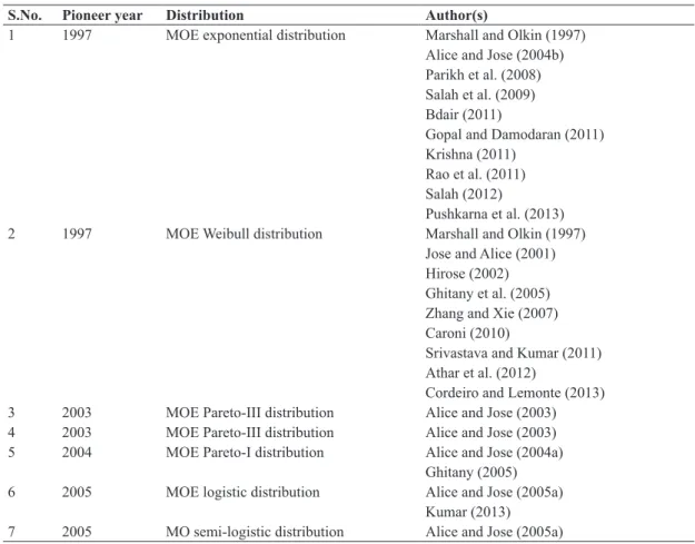
A list of papers on the MOE family is presented in Table II.
TABLE II
Contributed work on the MOE family of distributions.
S.No. Pioneer year Distribution Author(s)
1 1997 MOE exponential distribution Marshall and Olkin (1997) Alice and Jose (2004b) Parikh et al. (2008) Salah et al. (2009) Bdair (2011)
Gopal and Damodaran (2011) Krishna (2011)
Rao et al. (2011) Salah (2012)
Pushkarna et al. (2013) 2 1997 MOE Weibull distribution Marshall and Olkin (1997)
Jose and Alice (2001) Hirose (2002) Ghitany et al. (2005) Zhang and Xie (2007) Caroni (2010)
Srivastava and Kumar (2011) Athar et al. (2012)
Cordeiro and Lemonte (2013) 3 2003 MOE Pareto-III distribution Alice and Jose (2003) 4 2003 MOE Pareto-III distribution Alice and Jose (2003) 5 2004 MOE Pareto-I distribution Alice and Jose (2004a)
Ghitany (2005) 6 2005 MOE logistic distribution Alice and Jose (2005a)
S.No. Pioneer year Distribution Author(s)
8 2005 MO semi-Weibull distribution Alice and Jose (2005b) Thomas and Jose (2005) 9 2005 MOE Fréchet distribution Jose and Alice (2005)
Krishna (2011) Krishna et al. (2013) 10 2007 MOE Lomax distribution Ghitany et al. (2007) Gupta et al. (2010) 11 2007 MOE linear failure rate distribution Ghitany and Kotz (2007) 12 2007 MOE gamma distribution Ristić et al. (2007)
Jose (2009) 13 2008 MOE q-Weibull distribution Naik et al. (2008)
Jose et al. (2010)
14 2008 MOE Burr distribution Jayakumar and Mathew (2008) El-Bassiouny and Abdo (2010) 15 2008 MOE semi-Burr distribution† Jayakumar and Mathew (2008) 16 2008 MOE semi-Pareto III distribution† Jayakumar and Mathew (2008) 17 2009 MOE Linnik distribution† Jose and Uma (2009)
18 2009 MOE Mittag-Leffler distribution† Jose and Uma (2009) 19 2009 MOE beta distribution Jose et al. (2009) 20 2011 MOE uniform distribution Krishna (2011)
Jose and Krishna (2011)
21 2011 MOE Gumbel distribution Jose (2011)
22 2011 MOE generalized asymmetric Laplace
distribution† Krishna (2011)
Krishna and Jose (2011)
24 2013 MOE Zipf distribution P´erez-Casany and Casellas (2013) 25 2013 MOE power log-normal distribution Gui (2013a)
26 2013 MOE log-logistic distribution Gui (2013b) 27 2013 MOE quasi-Lindley distribution Gui (2013c) 28 2013 MOE Esscher transformed Laplace
distribution† George and George (2013)
† MO extension based on cf.
TABLE II (continuation)
BETA DISTRIBUTIONS AND EXISTING BETA G FAMILIES OF DISTRIBUTIONS
Consider the cdf of a beta random variable of type 1 with two shape parameters
a
and
b
given by
(4.1)
F
B1(
x
) =
P(X ≤ x)
=
I
x(
a
,
b
) =
B
x(
a
,
b
)
=
1
Z
0 x
x
a − 1(1 −
x
)
b − 1dx
,
B
(
a
,
b
)
B
(
a
,
b
)
where
a
> 0,
b
> 0,
x
2
(0, 1), B
t(
a, b
) =
Z
0 t
t
a − 1(1 −
t
)
b − 1dt
is the incomplete beta function,
It
(
a
,
b
) is the
incomplete beta function ratio and
B
(
a
,
b
) =
Z
0 1
t
a − 1(1 −
t
)
b − 1dt =
Γ
(
a
) Γ
(
b
)
Γ
(
a
+
b
)
is the beta function.
The pdf corresponding to (4.1) is
f
B1(
x
)
=
1
x
a − 1(1 −
x
)
b − 1,
B
(
a
,
b
)
Similarly, the cdf of a beta random variable of type 2 with parameters
a
and
b
is
(4.2)
F
B2(
y
) =
P
(Y ≤
y =
I
2
y(
a
,
b
) =
B2
y(
a
,
b
)
=
1
Z
0 y
y
a − 1dy
,
B2
(
a
,
b
)
B2
(
a
,
b
)
(1 +
y
)
a + bwhere
a
> 0,
b
> 0,
y
> 0,
B
2
t(
a
,
b
)
Z
0 t
t
a − 1(1 +
t
)
− (a + b)dt
is the incomplete beta function,
I
2
t(
a
,
b
) is the
incomplete beta function ratio and
B
2 (
a
,
b
) =
Z
0
∞
t
a − 1(1 +
t
)
− (a + b)dt =
Γ
(
a
) Γ
(
b
)
Γ
(
a
+
b
)
is the beta function.
The pdf corresponding to (4.2) is
f
B2(
y
),
=
1
y
a − 1
,
B
2 (
a
,
b
) (1 +
y
)
(a + b)where
a
> 0,
b
> 0, and
y
> 0. The beta type 2 distribution is also known as inverted beta distribution as it
can be obtained from (4.1) by the transformation
Y =
1 − XX.
Cardeño et al. (2005) introduced the beta type 3 distribution by transforming
Z =
2 − YYin (4.1).
The cdf of a beta random variable of type 3 with parameters
a
and
b
is
(4.3)
F
B3(
z
) =
P
(
Z
≤
z
) = 13
z
(
a
,
b
) =
B
3
z(
a
,
b
)
=
1
Z
0 z
z
a − 1(1 −
z
)
b − 1dz
,
B
3 (
a
,
b
)
B
3 (
a
,
b
)
(1 +
z
)
(a + b)where
a >
0,
b >
0,
z
2
(0
,
1),
B
3
t(
a, b
) =
Z
0 t
t
a − 1(1−
t
)
b − 1(1+
t
)
− (a + b)dt
is the incomplete beta function,
I
3
t
(
a, b
) is the incomplete beta function ratio and
B
3(
a, b
) =
Z
0 1
t
a − 1(1−
t
)
b − 1(1+
t
)
− (a + b)dt
=
Γ(
Γ(
a
) Γ(
b
)
a
+
b
)
is the beta function. The pdf corresponding to (4.3) is
f
B3(
z
)
=
2
az
a − 1(1 −
z
)
b − 1,
B
3 (
a
,
b
)
(1 +
z
)
(a + b)where
a >
0,
b >
0, and
z
2
(0
,
1).
Eugene et al. (2002) and Jones (2004a) replaced the upper limit
x
of the integral in (4.1) with
G
(
x
).
The resulting cdf of beta
G
family of distributions is
F
BG(
x
) =
I
G(x)
(
a, b
) =
B
G(x)(
a
,
b
)
B
(
a
,
b
)
=
1
B
(
a
,
b
)
Z
0 G(x)
!
a − 1(1−
!
)
b − 1d
!
.
(4.4)
The pdf corresponding to (4.4) is
(4.5)
f
BG(
x
) =
1
B
(
a
,
b
)
g
(
x
)
G
(
x
)
a − 1
[1−
G
(
x
)]
b − 1,
where
g
(
x
) =
dG
(
x
)
/dx
denotes the pdf. The beta
G
family of distributions is also known as the beta logit
family. For any lifetime random variable
t
, the sf, hrf, rhrf and chrf associated with (4.4) and (4.5) are
F
(
t
) = 1 −
I
G(x)(
a, b
) =
B
(
a
,
b
) −
B
G(t)(
a
,
b
)
B
(
a
,
b
)
,
h
(
t
) =
g
(
t
)
G
(
t
)
a −1
[1 −
G
(
t
)]
b −1B
(
a
,
b
) [
IG(
t)(
a
,
b
)]
=
g
(
t
)
G
(
t
)
a −1
[1 −
G
(
t
)]
b −1BG(
t)(
a
,
b
)
r
(
t
) =
g
(
t
)
G
(
t
)
a −1
[1 −
G
(
t
)]
b −1B
(
a
,
b
) [1 −
I
G(t)(
a
,
b
)]
=
g
(
t
)
G
(
t
)
a −1
[1 −
G
(
t
)]
b −1[
B
(
a
,
b
) −
B
G(t)(
a
,
b
)]
,
and
H
(
t
) = −log
B
(
a
,
b
) −
B
G(t)(
a
,
b
)
B
(
a
,
b
)
.
A list of papers on the beta
G
family of distributions is given in Table III.
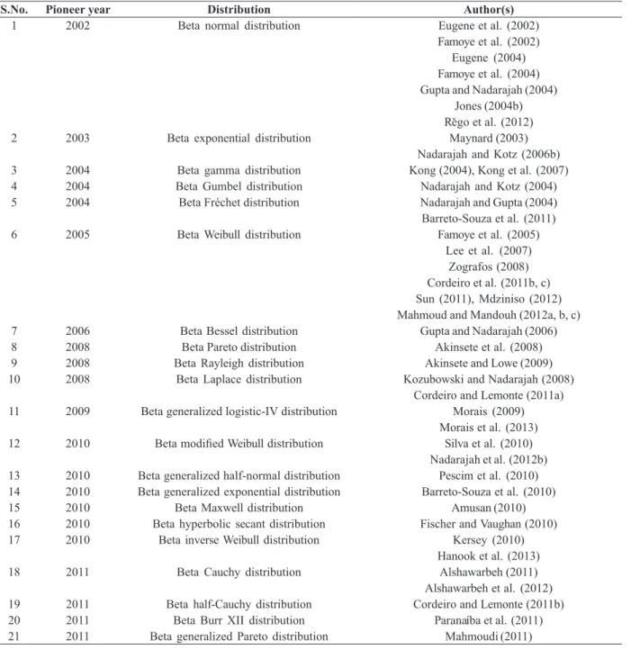
TABLE III
Contributed work on the beta Gfamily of distributions.
S.No. Pioneer year Distribution Author(s)
1 2002 Beta normal distribution Eugene et al. (2002)
Famoye et al. (2002) Eugene (2004) Famoye et al. (2004) Gupta and Nadarajah (2004)
Jones (2004b)
Rˇego et al. (2012)
2 2003 Beta exponential distribution Maynard (2003)
Nadarajah and Kotz (2006b)
3 2004 Beta gamma distribution Kong (2004), Kong et al. (2007)
4 2004 Beta Gumbel distribution Nadarajah and Kotz (2004)
5 2004 Beta Fréchet distribution Nadarajah and Gupta (2004)
Barreto-Souza et al. (2011)
6 2005 Beta Weibull distribution Famoye et al. (2005)
Lee et al. (2007) Zografos (2008) Cordeiro et al. (2011b, c)
Sun (2011), Mdziniso (2012)
Mahmoud and Mandouh (2012a, b, c)
7 2006 Beta Bessel distribution Gupta and Nadarajah (2006)
8 2008 Beta Pareto distribution Akinsete et al. (2008)
9 2008 Beta Rayleigh distribution Akinsete and Lowe (2009)
10 2008 Beta Laplace distribution Kozubowski and Nadarajah (2008) Cordeiro and Lemonte (2011a) 11 2009 Beta generalized logistic-IV distribution Morais (2009)
Morais et al. (2013)
12 2010 Beta modified Weibull distribution Silva et al. (2010)
Nadarajah et al. (2012b) 13 2010 Beta generalized half-normal distribution Pescim et al. (2010) 14 2010 Beta generalized exponential distribution Barreto-Souza et al. (2010)
15 2010 Beta Maxwell distribution Amusan (2010)
16 2010 Beta hyperbolic secant distribution Fischer and Vaughan (2010)
17 2010 Beta inverse Weibull distribution Kersey (2010)
Hanook et al. (2013)
18 2011 Beta Cauchy distribution Alshawarbeh (2011)
Alshawarbeh et al. (2012) 19 2011 Beta half-Cauchy distribution Cordeiro and Lemonte (2011b)
20 2011 Beta Burr XII distribution Parana´ıba et al. (2011)
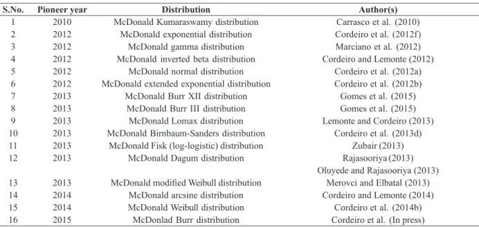
MCDONALD DISTRIBUTIONS AND MCDONALD G FAMILIES OF DISTRIBUTIONS
MCDONALD TYPE DISTRIBUTIONS
McDonald (1984) replaced the upper limit
x
of the integral in (4.1) with
x
c, where
c
is an additional (third)
shape parameter. The resulting cdf of the McDonald type (Mc) distribution is
(5.1)
F
(
x
) =
I
xc(
a
,
b
) =
B
xc(
a
,
b
)
=
1
Z
0 xc
x
a − 1(1 −
x
)
b − 1dx
,
B
(
a
,
b
)
B
(
a
,
b
)
where
a
> 0,
b
> 0 and
c
> 0 are the three shape parameters. The Mc distribution includes as special cases the
beta type 1 distribution (
c
= 1) and the Kumaraswamy distribution (
a
= 1). The pdf corresponding to (5.1) is
f
(
x
)
=
c
x
ac − 1(1 −
x
c)
b − 1,
B
(
a
,
b
)
where 0 <
x
< 1.
EXISTING MCDONALD GFAMILY OF DISTRIBUTIONS
For any baseline cdf
G
(
x
), Alexander et al. (2012) replaced the upper limit
x
cof the integral in (5.1) with
G
(
x
)
c. Lemonte and Cordeiro (2013) stated that this simple transformation facilitates the computation
of several properties of the
G
family of distributions.
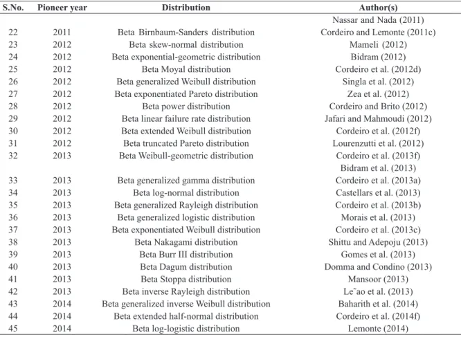
TABLE III (continuation)
S.No. Pioneer year Distribution Author(s)
Nassar and Nada (2011) 22 2011 Beta Birnbaum-Sanders distribution Cordeiro and Lemonte (2011c)
23 2012 Beta skew-normal distribution Mameli (2012)
24 2012 Beta exponential-geometric distribution Bidram (2012)
25 2012 Beta Moyal distribution Cordeiro et al. (2012d)
26 2012 Beta generalized Weibull distribution Singla et al. (2012) 27 2012 Beta exponentiated Pareto distribution Zea et al. (2012)
28 2012 Beta power distribution Cordeiro and Brito (2012)
29 2012 Beta linear failure rate distribution Jafari and Mahmoudi (2012) 30 2012 Beta extended Weibull distribution Cordeiro et al. (2012f) 31 2012 Beta truncated Pareto distribution Lourenzutti et al. (2012) 32 2013 Beta Weibull-geometric distribution Cordeiro et al. (2013f)
Bidram et al. (2013) 33 2013 Beta generalized gamma distribution Cordeiro et al. (2013a) 34 2013 Beta log-normal distribution Castellars et al. (2013) 35 2013 Beta generalized Rayleigh distribution Cordeiro et al. (2013b) 36 2013 Beta generalized logistic distribution Morais et al. (2013) 37 2013 Beta exponentiated Weibull distribution Cordeiro et al. (2013c)
38 2013 Beta Nakagami distribution Shittu and Adepoju (2013)
39 2013 Beta Burr III distribution Gomes et al. (2013)
40 2013 Beta Dagum distribution Domma and Condino (2013)
41 2013 Beta Stoppa distribution Mansoor (2013)
42 2013 Beta inverse Rayleigh distribution Le˜ao et al. (2013) 43 2014 Beta generalized inverse Weibull distribution Baharith et al. (2014) 44 2014 Beta extended half-normal distribution Cordeiro et al. (2014f)