Abstract—It is well known that the stochastic nature of the
interference deeply impacts the performance of emerging and future wireless communication systems. In this work we consider an ad hoc network where the nodes move according to the Random Waypoint mobility model. Assuming a time-varying wireless channel due to slow and fast fading and, considering the dynamic path loss due to the mobility of the nodes, we start by characterizing the interference distribution caused to a receiver by the moving interferers located in a ring. For this purpose, we consider a receiver located at the center of the simulated region. Based on the distribution of the interference’s power, we evaluate different methodologies to estimate the power of the interference in real-time. Results achieved with a Maximum Log-likelihood estimator (MLE) and a Probability Weighted Moments (PWM) estimator are compared. The accuracy of the results achieved with the proposed methodologies in several simulations show that they may used as an effective tool of interference power estimation in future wireless communication systems, exhibiting high accuracy even when the number of samples is low.
Keywords— Interference Estimation, Ad Hoc Networks,
Mobility.
I. INTRODUCTION
HE characterization of the interference in wireless networks plays an important role in several applications, ranging from localization [1], security [2], spectrum sensing [3] and others. In the majority of wireless scenarios the characterization of the aggregate interference is a complex task. Aggregate interference caused by multiple nodes spatially distributed in a given area is mainly due to the wireless propagation effects, especially: the attenuation of the signal with distance (path loss); the obstruction of the propagation path between transmitter and receiver by large objects (shadowing or slow fading); and the reflection of the propagated signal resulting in the reception of multiple copies of the same transmitted signal (fast fading or multipath fading).
Paper received June 14, 2016; accepted October 6, 2016. Date of publication November 20, 2016. The associate editor coordinating the review of this manuscript and approving it for publication was Prof. Aleksandar Nešković.
This paper is a revised and expanded version of the paper presented at the 23rd Telecommunications Forum TELFOR 2014 [20].
This work was partially supported by the Portuguese Science and Technology Foundation (FCT/MEC) under the grant SFRH/BD/108525/2015.
The authors are with Instituto de Telecomunicações - IT, Av. Rovisco Pais, 1, 1049 - 001 Lisboa - Portugal and CTS, UNINOVA, Dep.º de Eng.ª Electrotécnica, Faculdade de Ciências e Tecnologia, FCT, Universidade Nova de Lisboa, 2829-516 Caparica, Portugal.
E-mail: [email protected], [email protected].
Although the aggregate interference is often caused by a high number of nodes, and thus the central limit theorem (CLT) applies, most of the times CLT cannot be used due to the existence of dominant interferers [16].
While several authors model the aggregate interference in static networks [4], the assumption of nodes’ mobility introduces a novel degree of uncertainty related with the position of the nodes and their level of mobility. The works already published approaching the characterization of the interference in mobile networks are mainly focused on interference modeling. The use of statistical information related with the mobility of the interferers in the interference modeling was carried out in a few and very recent works [5]–[7].
In [5] the aggregate interference caused by static nodes (cells) is characterized for the uplink channel of a single terminal moving according to a random pattern. In this case the interference is caused by static nodes and the terminal mobility only causes a time-varying displacement with respect to different cells. The work in [6] considers an ad hoc network scenario where the nodes move according to the random direction model (RD). The probability density function (PDF) of the distance between any pair of nodes is used to characterize the aggregate interference due to path loss. Because a static receiver is assumed in the RD model, the distance variables between interferers and the receiving node are independent, and the CLT applies. In this case, a Gaussian modeling approach is used. [7] assumes that the interferers may move according to the random waypoint mobility model (RWP). Differently from the RD uniform model, in the RWP model the vertical and horizontal components of the nodes’ position may be slightly correlated [10], and the assumptions considered in [6] for the RD model do not hold for the RWP model. Consequently, to deduce the path loss interference, [7] only considers the contribution from the nearest interferer to the receiver, neglecting the contribution of the nodes farther away. Recently, we have proposed an interference model for ad hoc networks where the nodes move according to the RWP and all the contributions of the nodes located within a defined region are considered [8]. Differently from [7], in [8] we model the aggregate interference considering the contribution of multiple nodes acting as interferers.
The estimation of the interference caused by multiple nodes transmitting in the neighborhood of a receiving node has been studied in a few scenarios. [17] proposes a method of interference estimation for CDMA systems where, knowing prior statistical knowledge of interference, it is possible to determine the coefficients of an estimator
Interference Estimation in Wireless Mobile
Random Waypoint Networks
Luis Irio, Daniela Oliveira, and Rodolfo Oliveira, SeniorMember, IEEE
by solving a set of linear equations. The authors propose a model for the system and its performance analysis is evaluated through the expected value of the estimation error and the approximate expression for the probability of error. [18] approaches the interference estimation for multi-layer multi-user multiple-input and multiple-output (ML-MU-MIMO) transmission for LTE-Advanced (long term evolution) systems. In this work the authors admit a User-specific reference signal (UE-RS) and investigate various interference covariance estimation schemes in LTE-Advanced systems. [18] shows the significant influence of the interference estimation schemes on the system performance at the link level. In [19] the authors consider a new interference estimation scheme for a wireless femto cell system, which is surrounded by other femto cells using the same band.
In this work we start by characterizing the distribution of the interference caused to a receiver by multiple moving nodes located in a ring, considering path loss and slow and fast fading. Based on the interference distribution, we evaluate two different methodologies to estimate the interference in real-time. The proposed methodologies are evaluated through simulation. Finally, several scenarios are discussed and the achieved results for each one of them are presented in order to assess its accuracy. The main contribution of this work is the identification of a method to estimate the aggregate interference in random waypoint mobility networks, leading to accurate results when used in real-time.
The paper is organized as follows. Section II presents the general assumptions considered in this work. In Section III the distribution of the interference values obtained through simulation is approximated by known distributions in order to identify possible approximations. Section IV describes two estimation methodologies as well as the real-time estimates obtained through simulation. Finally, Section V concludes the paper by outlining its contribution.
II. SYSTEM DESCRIPTION
A. Mobility Assumptions
In this work we consider that nodes move according to the RWP mobility model [9]. In a RWP mobility model each node is initially placed in a random position ( , ). The position is sampled from the uniform distributions represented by ∈ 0, and ∈ 0, . ( , ) represents the starting point, and the next step is to define the ending point ( , ), which is also uniformly chosen as the starting point (i.e. ∈ 0, and ∈ 0, ). Then a node uniformly chooses the velocity ∈
, to move from the starting point to the ending point. After reaching the ending point ( , ), a node randomly chooses a pause duration ( ), and during this period of time it remains stopped in the ending point. After elapsing , a node uniformly chooses a new velocity value to move to another ending point uniformly chosen. After reaching the ending point a node repeats the same cycle as many times as required.
Considering that E represents the expected distance
between two random points and E represents the expected velocity of the nodes without considering pause, the expected velocity of the nodes considering pause is given by
E = , (1)
where E and E are defined in [10] as
E = ( / ) ,
E 521.405m, and E represents the expected value of the pause duration.
B. Network Scenario
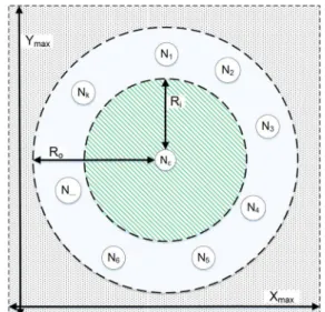
The network scenario considered in this work assumes a RWP mobility scenario where nodes move in a region defined by the area × . The network model considered in this work is illustrated in Figure 1. A fixed central node is located in the center of the scenario (in the position ( ⁄ ,2 ⁄2)), which operates as a fixed receiver of the mobile transmitting nodes. The objective of this paper is the characterization and estimation of the aggregate interference caused to by the hypothetical transmitters , , … , located within the interference region, i.e., the mobile transmitters located within the ring bounded by the smaller circle of radius and the larger circle of radius . The parameters describing the network and the mobility conditions are described in Table 1.
Fig. 1 Aggregate interference sensed by due to the hypothetical mobile interferers located in the annulus area
( − ).
TABLE 1:PARAMETERS ADOPTED IN THE SIMULATIONS.
1000 m 100
1000 m 0 s ; 300 s Simulation
time 3000 s 20 m
5 m/s 120 m
C. Radio Propagation Assumptions
This subsection describes the radio propagation scenario considered in this work. The total interference power received by the node located in the centre is expressed by
= ∑ , (2)
where is the interference caused by the i-th node, and is the total number of nodes located in the ring area ( − ). The interference power is given by
= , (3)
where is the transmitted power level of the i-th node ( = 10 mW is assumed for each node). represents the fading observed in the channel between the receiver and node and is the distance between the i-th interferer and the receiver. represents the path-loss coefficient. No power control is applied.
The fading includes the small-scale fading and shadowing effects. The small-scale fading effect is assumed to be distributed according to a Rayleigh distribution, which is represented by
( ) = , (4)
where is the envelope amplitude of the received signal, and 2 is the mean power of the multipath received signal. = 1 is adopted in this work.
Regarding the fading effect, we have assumed that it follows a Lognormal distribution
( ) =√
( ( ) )
, (5)
where is the shadow standard deviation when = 0. The standard deviation is usually expressed in decibels and is given by = 10 ⁄ln(10). For → 0, no shadowing results. Although (5) appears to be a simple expression, it is often inconvenient when further analyses are required. Consequently, [11] has shown that the log-normal distribution can be accurately approximated by a gamma distribution, defined by
( ) = ( ) , (6)
where is equal to 1 − 1 and is equal to ( + 1)⁄ . Γ(. ) represents the Gamma function.The probability distribution function of the fading is thus represented by
( ) = ( ) , (7)
which is the Generalized-K distribution, where (. ) is the modified Bessel function of the second kind.
III. CHARACTERIZATION OF THE INTERFERENCE
DISTRIBUTION
Following the assumptions considered in the previous section, several simulations were performed considering different propagation and mobility conditions. Regarding the mobility conditions two different scenarios were defined:
• Mobility scenario 1 - = 5m/s, =
20m/s, and = 0s, representing an average node's velocity E = 10.82 m/s;
• Mobility scenario 2 - = 5m/s, =
20m/s, and = 300s, representing an average node's velocity E = 1.50 m/s.
•
Regarding the propagation conditions, three different scenarios were defined representing different path loss coefficients and fading variance:
• Radio scenario 1 – = 2 and = 3dB; • Radio scenario 2 – = 4 and = 3dB; • Radio scenario 3 – = 2 and = 6dB.
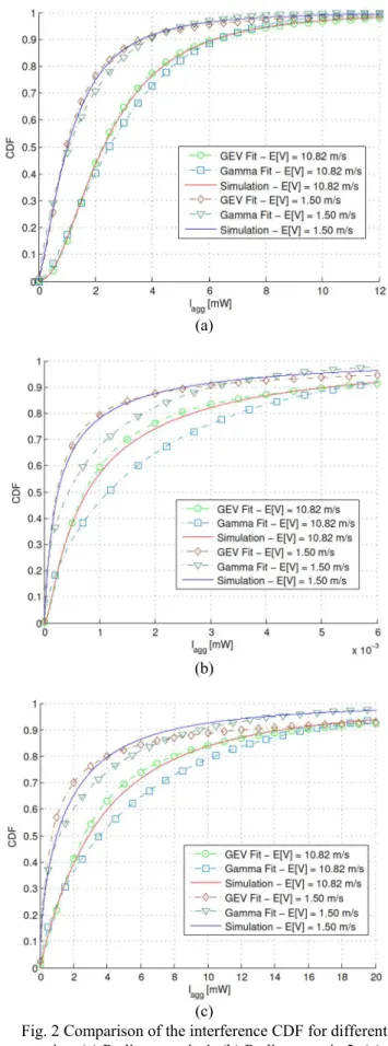
During the simulations, the interference power sensed by the node was sampled every second in order to compute its Cumulative Distribution Function (CDF). Figure 2 presents the results computed from the simulation data (“Simulation” curve represented in the figure). The samples acquired in 1000 simulations of 3000 seconds, totaling a sample set of = 3 × 10 samples, were also used to determine the parameters of a set of different probability density functions (PDFs) using a maximum-likelihood (ML) fitting methodology. For each one of the considered PDF , an average logarithm likelihood was defined as follows
= ∑ ln ( |Θ) , (8)
whereΘ represents the parameters of the PDF and represents each individual sample. ML was used to maximize the likelihood in order to determine Θ, which is described as follows
Θ = argmax (Θ; , … , ) . (9)
Figure 2 represents the CDFs computed with the parameters obtained in (9) for the Generalized Extreme Value (GEV) and Gamma distributions. As illustrated, the fitting obtained with the GEV distribution presents a better approximation for the different mobility and radio propagation conditions. Because of this observation, the estimation methods proposed in the next section assume that the interference distribution follows a GEV distribution.
IV. INTERFERENCE ESTIMATION
(a)
(b)
(c)
Fig. 2 Comparison of the interference CDF for different scenarios: (a) Radio scenario 1; (b) Radio scenario 2; (c)
Radio scenario 3.
( ; , , ) = ( ) ( ) , (10)
where
( ) = 1 + , 0
( )⁄ , = 0 . (11) A Maximum Log-likelihood estimator (MLE) and a Probability Weighted Moments (PWM) estimator are introduced in the next subsections, in order to be used in real time to estimate the aggregate interference. Hereafter, we denote the elements of an interference sample set by = , , … , . We also consider the ordered sample set, which is denoted by , ⋯ , .
A. Log-Likelihood Estimator
The log-likelihood function for a sample set = , … , of i.i.d GEV random variables is given by
( , , ) ∑
∑ (12)
under the condition 1 + 0. The MLE estimator ( , , ̂) for ( , , ) is obtained by maximizing (12).
B. PWM Estimator
As described in [13], the PWM of a random variable with distribution function ( ) = ( ) are the quantities
, , = E (X) 1 − (X) , (13)
for real , and values. For the GEV distribution, [14] shows that E (X) can be written as
, , = − 1 − ( + 1) Γ(1 − ) , (14) with 1 and 0.The PMW estimators ( , , ̂) of the GEV parameters ( , , ) are the solution of the following system of equations
, , = − (1 − Γ(1 − )) 2 , , − , , = Γ(1 − ) (2 − 1)
, , , , , , , , =
, (15)
in which , , can be replaced by the unbiased estimator proposed in [15]
, , = ∑ ∏ , . (16)
C. Simulation Results
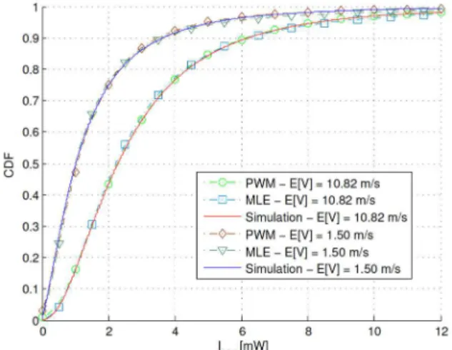
presented in Figure 3 is the average of the 20 CDFs computed for each sample set. The correlation of the samples of each sample set was in the interval [0.9020, 0.9339].
Fig. 3 Simulation results obtained with the MLE and PWM estimators for Radio scenario 1.
Regarding the accuracy of the proposed estimators, for the radio scenario 1 considered in Figure 3 both MLE and PWM estimators present high accuracy. This fact is due to the standard deviation value σξdB. For higher values of σξdB, the accuracy of the PWM estimator is higher than the MLE. From the results depicted in Figure 3, we may observe that the accuracy of the estimators is maintained for different mobility parameters. As a final remark, the results presented in Figure 3 validate the proposed estimation methodologies, being the PWM estimator more adequate for the real-time estimation due to its higher accuracy. Finally, we highlight that approximate results were observed for smaller sample set sizes using the PWM estimator, and similar results may be achieved using only m = 10 samples per sample set, which is a remarkably low number of samples.
V. CONCLUSIONS
In this work we consider an ad hoc network where the nodes move according to the Random Waypoint mobility model. Assuming a time-varying wireless channel due to slow and fast fading and, considering the dynamic path loss due to the mobility of the nodes, we start by characterizing the interference distribution caused to a receiver by the moving interferers located in a ring. The simulation results confirm that the distribution of the aggregated interference may be accurately approximated by a Generalized Extreme Value distribution. Based on the interference distribution, two different methodologies based on a MLE and a PWM estimators were assessed to estimate the interference in real-time. The accuracy of the results achieved with the proposed methodologies shows that they may used as an effective tool of interference estimation in future wireless communication systems. Moreover, the low number of required samples constitutes one of the advantages of the proposed PWM estimator, even when the samples are highly correlated.
REFERENCES
[1] K. Pahlavan, X. Li and J.-P. Makela,“Indoor Geolocation Science and Technology,” IEEE Commun. Mag.,vol. 40, no. 2, pp. 112–118,
Feb. 2002.
[2] S. Goel and R. Negi,“Guaranteeing Secrecy using Artificial Noise,”
IEEE Trans. Wireless Commun., vol. 7, no. 6, pp. 2180–2189, June
2008.
[3] A. Rabbachin, T.Q.S. Quek, H. Shin and M.Z. Win,“Cognitive Network Interference,”IEEE J. Sel. Areas Commun., vol. 29, no. 2,
pp. 480–493, Feb. 2011.
[4] M.Z. Win, P.C. Pinto and L.A. Shepp,“A Mathematical Theory ofNetwork Interference and Its Applications,”Proceedings of the IEEE,vol. 97, no. 2, pp. 205–230, Feb. 2009.
[5] S. Yarkan, A. Maaref, K. H. Teo and H. Arslan, “Impact of Mobility on the Behavior of Interference in Cellular Wireless Networks,” inIEEE GLOBECOM 2008, New Orleans,2008, pp. 1–
5.
[6] X.M. Zhang, L. Wu, Y. Zhang and D.K. Sung,“Interference dynamics in MANETs with a random direction node mobility model,” in IEEE Wireless Communications and Networking Conference (WCNC), Shanghai, 2013, pp. 3788–3793.
[7] Z. Gong and M. Haenggi, “Interference and Outage in Mobile Random Networks: Expectation, Distribution, and Correlation,”IEEE Trans. MobileComput.,vol.13, no. 2, pp. 337–
349, Feb. 2014.
[8] L. Irio, R. Oliveira and L. Bernardo,“Aggregate Interference in Random Waypoint Mobile Networks,” IEEE Commun. Lett., vol.
19, no. 6, pp. 1021-1024, June 2015.
[9] D.B. Johnson and D.A.Maltz, “Dynamic Source Routing in Ad Hoc Wireless Networks,” inMobile Computing, Springer, 1996, pp.153–
181.
[10] C. Bettstetter, G. Resta, and P. Santi, “The node distribution of the randomwaypoint mobility model for wireless ad hoc networks,”
IEEE Trans. Mobile Comput., vol. 2, no. 3, pp. 257-269, July 2003.
[11] A. Abdi and M. Kaveh,“On the utility of gamma PDF in modeling shadowfading (slow fading),” in IEEE Vehicular Technology Conference, Houston, 1999, pp. 2308–2312.
[12] S.A. Ahmadi and H.Yanikomeroglu, “On the approximation of the generalized-K distribution by a gamma distribution for modelingcomposite fading channels,”IEEE Trans. Wireless Commun., vol. 9, no. 2, pp.706–713, Feb. 2010.
[13] J.A. Greenwood, J.M. Landwehr, N.C. Matalas andJ.R. Wallis,“Probability weighted moments: Definition and relationto parameters of several distributions expressable in inverse form,”
Water Resources Research, vol. 15, no. 5, pp. 1049–1054, Oct.
1979.
[14] J.R.M. Hosking, J.R. Wallis and E.F. Wood,“Estimation of the Generalized Extreme-Value Distribution by the Method of Probability-Weighted Moments,”Technometrics, vol. 27, no. 3, pp.
251–261, Aug.1985.
[15] J.M.Landwehr, N.C. Matalas and J.R. Wallis“Probability weightedmoments compared with some traditional techniques in estimating GumbelParameters and quantiles,” Water Resources Research, vol. 15, no. 5, pp. 1055–1064, Oct. 1979.
[16] M. Chiani. Analytical distribution of linearly modulated cochannel interferers. Communications, IEEE Transactions on, 45(1):73–79, Jan 1997.
[17] M. R. Shikh-Bahaei and A. H. Aghvami, "An interference estimation method for interference cancellation in CDMA systems," CDMA Techniques and Applications for Third Generation Mobile Systems (Digest No.: 1997/129), IEE Colloquium on, pp. 4/1-4/6, London, 1997.
[18] Z. Bai et al., "Interference estimation for multi-layer MU-MIMO transmission in LTE-Advanced systems," 2012 IEEE 23rd International Symposium on Personal, Indoor and Mobile Radio Communications - (PIMRC), Sydney, pp. 1622-1626, NSW, 2012. [19] W. Lee and D. H. Cho, "Adaptive interference estimation for
directional transmission," 2012 IEEE Consumer Communications and Networking Conference (CCNC), pp. 350-351, Las Vegas, NV, 2012.