Digital Object Identifier (DOI) 10.1007/s00220-016-2677-9
Mathematical
Physics
Anosov Diffeomorphisms and
γ
-Tilings
João P. Almeida1 , Alberto A. Pinto2
1 LIAAD–INESC TEC and Department of Mathematics, School of Technology and Management, Polytechnic Institute of Bragança, Campus de Santa Apolónia, 5300-253 Bragança, Portugal. E-mail: [email protected]
2 LIAAD–INESC TEC and Department of Mathematics, Faculty of Sciences, University of Porto, Rua do Campo Alegre n. 687, 4169-007 Porto, Portugal. E-mail: [email protected]
Received: 26 July 2013 / Accepted: 18 April 2016
Published online: 14 June 2016 – © Springer-Verlag Berlin Heidelberg 2016
Abstract: We consider a toral Anosov automorphism Gγ : Tγ → Tγ given by Gγ(x,y) = (ax + y,x)in the < v, w > base, where a ∈ N\{1}, γ = 1/(a +
1/(a + 1/ . . .)), v = (γ ,1) and w = (−1, γ ) in the canonical base of R2 and
Tγ = R2/(vZ×wZ). We introduce the notion ofγ-tilings to prove the existence of
a one-to-one correspondence between (i) marked smooth conjugacy classes of Anosov diffeomorphisms, with invariant measures absolutely continuous with respect to the Lebesgue measure, that are in the isotopy class ofGγ; (ii) affine classes ofγ-tilings; and (iii)γ-solenoid functions. Solenoid functions provide a parametrization of the infi-nite dimensional space of the mathematical objects described in these equivalences.
1. Introduction
This paper studiesC1+smooth conjugacy classes of Anosov diffeomorphismsGof the two-dimensional torus with a prescribed isotopy classGγ. The ispotopy classes treated here belong to a countable family, each of which is determined by a Fibonacci like matrix. Inspired in the works of Jiang [14] and Pinto and Sullivan [30], Pinto et al. [21] introduced the notion ofgolden tilingand proved the one-to-one correspondences claimed in the abstract of this paper for the usual Fibonacci matrix, i.e.a =1. Here, we extend their results for the case of Fibonacci like matrices, i.e. a ∈ N\{1}, by introducing theγ
-tilings. Like the golden tilings, theγ-tilings record the infinitesimal geometric structure along the unstable leafs that are invariant under the action ofG. The properties of theγ -tilings are given in a canonical way using theγ-Fibonacci decompositionof the natural numbers by the greedy algorithm (see [8]). The main contribution of this work consists in understanding the way thisγ-Fibonacci decomposition encodes the combinatorics determined by the Markov partition of G along the unstable leafs that are invariant under the action ofG(see Theorem2).
con-tinuous with respect to Lebesgue, that are in the isotopy class of Gγ; (ii)γ-tilings; and (iii)γ-solenoid functions. Hence, Theorem 3gives a characterization of marked smooth conjugacy classes of Anosov diffeomorphisms in terms of certain affine classes of tilings of the half-line by intervals. The tilings are essentially given by the tilings of the unstable manifold of a fixed point, obtained by considering its intersection with the rectangles in a canonical Markov partition. Theorem4is about rigidity: an Anosov diffeo-morphism, with an invariant measure absolutely continuous with respect to Lebesgue, whose unstable holonomies are of class C1+zi gmund, is necessarily conjugate to the affine representative. The proofs of these results follow closely those in [21]. One of the main ingredients in the proof of Theorem3is the solenoid function of an Anosov map (see [26,28]), which is similar to the scaling function of a hyperbolic Cantor set (see [7,33]). The ratios between the lengths of consecutive intervals in an admissible tiling are precisely the values of the solenoid function in a certain sequence of points. Since this sequence of points is dense in the domain of the solenoid function, the main problem is to determine the conditions for a sequence of values on this set to extend to a Hölder continuous solenoid function. This leads naturally to the matching, the bound-ary, and the exponentially fast repetitive conditions that give the definition of admissible tilings (see Sect.4.4). Section3contains most of the new combinatorial results needed to establish these conditions. Once Theorem3is established, Theorem4follows from known arguments.
As opposed to the case treated in [21], the Anosov automorphismGγ considered in this paper hasa ≥ 2 fixed points instead of a single one. These fixed points are dynamically indistinguishable from each other: for each pair of these fixed points there is an orientation preserving conjugacy mapping one of the fixed points to the other. An unstable leaf is invariant under the dynamics if, and only if, the leaf passes through a fixed point. Hence, there areaof such invariant leafs. We associate to each one of these leafs the correspondingγ-tiling. Hence, each Anosov diffeomorphism determines a set of γ-tilings with cardinality a. Hence, two Anosov diffeomorphisms, with invariant measures absolutely continuous with respect to Lebesgue, are smooth conjugate if, and only if, they determine the same sets ofγ-tilings. In fact, if two of these Anosov diffeomorphisms determine a sameγ-tiling, then they determine the same sets ofγ -tilings. Furthermore, we observe that a solenoid function determines a ratio function (see [26,28]) that measures the ratio of the asymptotic lengths of any pair of leaves with a common endpoint. Hence, any twoγ-tilings are obtained from the same Anosov diffeomorphism, but using unstable lines passing through different fixed points, if, and only if, they determine the same ratio function.
Every Anosov automorphism determines a rigid rotation that is a periodic orbit of a renormalization operator (see, for instance, [1,28]). Putting together the results in this paper and in Pinto et al. [21], all Anosov automorphisms determining rigid rotations that are fixed points of a renormalization operator are treated. An open problem consists in extending these results to the isotopy classes of Anosov automorphisms on surfaces whose rigid rotation is not a fixed point of a renormalization operator. Another open problem consists in understanding the tilings determined by the marking of the stable manifolds (without reversing the Markov partition and time).
2. Anosov Diffeomorphisms and Circle Rotations
We start by fixing an integera ∈N\{1}and consider the positive real number
γ =(−a+a2+ 4)/2=1/(a+ 1/(a+ 1/ . . .)).
We observe thatγsatisfies the key relationaγ+γ2=1. Letv=(γ ,1)andw=(−1, γ )
in the canonical base ofR2. LetTγ =R2/(vZ×wZ)be the quotient space with the quotient topology. We consider the Anosov automorphismGγ : Tγ → Tγ given by Gγ(x,y)=(ax+y,x)in the base< v, w >.
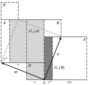
The eigenvalues ofGγ areμ− = −γ andμ+ = 1/γ. Letπγ : R2 → Tγ be the natural projection ofR2inTγ. Let A˜ = [0,1] × [0,1]andB˜ = [−γ ,0] × [0, γ]be rectangles in the planeR2. LetA=πγ(A˜)andB=πγ(B˜)be the projections ofA˜and
˜
Bin the torusTγ (see Fig.1). Thegenerating Markov partitionMGγ ofGγ is given byMGγ = {A,B}. The stable and unstable manifolds ofGγ are the projection byπγ
of the horizontal and vertical lines of the plane, respectively.
2.1. Marked Anosov diffeomorphisms. Let G be the set of all pairs (G,z) with the property that (i) for someα >0,G : T→ Tis aC1+α Anosov diffeomorphism in a two dimensional torusTwith an invariant measure absolutely continuous with respect
to Lebesgue measure; and (ii)zis a fixed point ofG. Hence, the tangent bundle ofGhas aC1+α uniformly hyperbolic splitting into a stable direction and an unstable direction and the holonomies areC1+α1 smooth, for some 0< α1≤α(see [19,28,32]). We call
(G,z)∈Gamarked C1+Anosov diffeomorphism, because we have marked one of its fixed points. LetGγ be the set of all pairs(G,z)∈ Gsuch that there is a topological conjugacy hG : Tγ → T between the Anosov automorphism Gγ and the Anosov diffeomorphismGsuch thatz=hG(πγ(0,0)). We note that the topological conjugacy hG, preserving the orientation, is uniquely determined. The generating Markov partition
M(G,z)of G is formed by the rectangles hG(A) andhG(B), where A and B are
Fig. 1.The generating Markov partitionMG
γ and the dynamics of the Anosov automorphismGγ for the
the rectangles of the generating Markov partitionMGγ of Gγ (see Sect.1). EveryG
topologically conjugatetoGγ determines exactlyamarked pairs(G,z1), . . . , (G,za),
wherez1, . . . ,zaare the fixed points ofG.
We say that two marked C1+ Anosov diffeomorphisms (G0,z0), (G1,z1) ∈ Gγ are marked smooth conjugate if the topological conjugacy h between G0 and G1,
withh(z0) = z1, is a C1+ diffeomorphism. The marked smooth conjugacy classof (G0,z0) ∈ Gγ consists of all (G1,z1) ∈ Gγ that are marked smooth conjugate to
(G0,z0). Hence, twoC1+Anosov diffeomorphismsG0andG1are smooth conjugate, if
there are fixed pointsz0ofG0andz1ofG1such that(G0,z0)and(G1,z1)are marked
smooth conjugate.
2.2. The rigid rotation g. Letπγ : R2 → Tγ be the natural projection, whereTγ =
R2/(vZ×wZ). LetS=R/[1 +γ]Zbe the anticlockwise oriented circle with the metric
induced by the Euclidean metric onR. LetπS :R→ Sbe the natural projection with the property that
πS(x)=πS(x+ 1 +γ ),
for everyx∈R. LetiS:πγ([−γ ,1] × {0})→Sbe the natural local inclusion with the property that
iS◦πγ(x,0)=πS(x).
We observe thatπγ(−γ ,0)=πγ(1,0), but
iS◦πγ(−γ ,0)=πS(−γ )=πS(1)=iS◦πγ(1,0).
Letg :S→Sbe the rigid rotation with anticlockwise rotation numberγ /(1 +γ ).
The mapghas the property that
g◦πS(x)=πS(x−γ ),
for everyx∈R.
3. Combinatorics and Geometry of the Tilings
In this section, we introduce the tilings and we show the relation between the combi-natorics of the tilings and the geometry connected with the Markov partitions of the Anosov diffeomorphims.
3.1. γ-Fibonacci decomposition. Theγ-Fibonacci sequenceis the sequence of natural numbers(Fn)n∈Ndefined recursively by
F0=1, F1=1, and Fn+2=a Fn+1+Fn, for n≥0.
Theγ-Fibonacci decomposition((an0,Fn0), . . . , (anp,Fnp))ofi∈N\{1}is given as follows (see the greedy algorithm in [8]): (i)Fn0andan0 ∈ {1, . . .a}are respectively the largest term in theγ-Fibonacci sequence and the largest integer such that the following inequality holds
(ii) proceeding inductively, fork∈N, let
Fn0 >· · ·>Fnk−1
anda0, . . . ,ank−1 ∈ {1, . . . ,a}be such that
an0Fn0+· · ·+ank−1Fnk−1 ≤i;
(iii) choose the largest term in theγ-Fibonacci sequence
1 +a =F2≤ Fnk <Fnk−1
and the largest integerank ∈ {1, . . . ,a}such that the following inequality holds
ankFnk ≤i−(an0Fn0+· · ·+ank−1Fnk−1);
(iv) hence, there exists a natural numberq∈N, such that
i=an0Fn0+· · ·+anqFnq +b,
where nq ≥ 2 andb ∈ {0,1, . . .a}; (v) now, we define the remaining terms of the γ-Fibonacci decomposition ofias follows:
(a) ifb=0 then p=q;
(b) ifb=1 andnqis odd thenp=q+ 1,np=0 andanp =1; (c) ifb=1 andnqis even thenp=q+ 1,np=1 andanp =1; and (d) ifb>1 then p=q+ 2,np−1=1,anp−1 =b−1,np=0 andanp =1.
Formally, we attribute to 0 the γ-Fibonacci decomposition (1,F0) and to 1 the γ
-Fibonacci decomposition(1,F1). We observe that F0 has a bivalent interpretation in
this paper,F0denotes 0, but values 1 when used in mathematical operations. Hence, the
sequence((an0,Fn0), . . . , (anp,Fnp))is aγ-Fibonacci decomposition corresponding to some natural numberi ∈N0if, and only if, for everyj ∈ {0, . . . ,p},
(i) anj ∈ {1, . . . ,a};
(ii) ifanj =a, thennj+1≥nj+ 2; (iii) ifnp=0, thenanp =1;
(iv) ifnp=0 andnp−1>1, thennp−1is odd; and
(v) ifnp=1, thenanp =1 andnp−1is even.
We observe that every natural numberi∈N0has a uniqueγ-Fibonacci decomposition. Theγ-Fibonacci shiftσ :N0→N0is defined by
σ (i)=an0Fn0+1+· · ·+anpFnp+1.
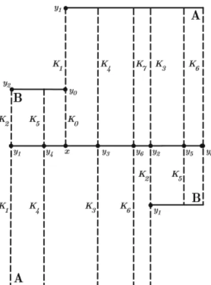
Fig. 2.The unstable leafW= ∪i≥0Kiand the boundary pointsyi−1andyiof the unstable spanning leafs
Ki, fori ≥2. We note thatK0is theright unstable boundaryof the generating Markovrectangle B, with endpointsxandy0;K1is theleft unstable boundaryof the generating Markovrectangle A, with endpointsx andy1, wherex=πγ(0,0)is the marked fixed point ofGγ
3.2. Combinatorics and geometry of the tilings. Let W0 = {(0,y) : y ≥ 0}be the
positive vertical axis ofR2. Hence, W = πγ(W0)is part of the unstable leaf of the automorphismGγ(see notations in Sect.2). The unstable leafW has only one endpoint x = πγ(0,0) that is a fixed point of Gγ. Let y0 = πγ(0, γ ), y1 = πγ(0,1)and y2=πγ(0,1 +γ ). LetK0⊂W be the unstable spanning leaf segment with boundary
pointsxandy0; letK1⊂Wbe the unstable spanning leaf segment with boundary points
xandy1; and letK2⊂W be the unstable spanning leaf segment with boundary points
y1andy2. Hence,K0⊂K1;K0is the right unstable boundary of the generating Markov
rectangleB;K1is the left unstable boundary of the generating Markov rectangleA;K2
is the left unstable boundary of the generating Markov rectangleB; and(K1∪K2)\K0is
the right unstable boundary of the generating Markov rectangle A. Lety3, y4, . . .∈Tγ andK3, K4, . . .∈ W be defined, inductively, as follows: for everyi ≥ 3, (i)Ki is an
unstable spanning leaf of a generating Markov rectangle; and (ii){yi−1} = Ki−1∩Ki
is a common boundary point of both Ki−1andKi (see Fig.2). Hence,W = ∪i≥1Ki,
iS(y0)=iS(y1),Gγ(y0)=y1, butGγ(y1)=y2becausea>1.
ThetilingLγ is the set
Lγ = {(Ki,Ki+1) ,i ∈N}.
Definition 1.In the tilingLγ, for everyi ∈N,
(i) ifKi ⊂AandKi+1⊂B, theni is of type(A,B);
(ii) ifKi ⊂BandKi+1⊂A, theni is of type(B,A); and
(iii) ifKi,Ki+1⊂A, theni is of type(A,A).
For simplicity of notation, we denoteπS(0)by 0. Letzi =iS(yi), for everyi ∈N.
Hence, by construction,z0=z1=g(0)andzi+1 =g(zi)=gi+1(0), for everyi ∈N.
Furthermore,
Fig. 3. The mapπS(w)=iS◦πγ(w,0)|[−γ ,1], for everyw∈ [−γ ,1], and the pointszi=iS(yi)=πS(wi),
fori∈N. We note thatz0=iS(x)=πS(0)
where ((an0,Fn0), . . . , (anp,Fnp)) is theγ-Fibonacci decomposition ofi ∈ N0 (see Fig.3). Let us denote byℓ(x,yi)the leaf segment with endpointsxandyi. LetmA(i)be
the number of spanning leaf segments of the Markov rectangle AinLγ that belong to
ℓ(x,yi); and letmB(i)be the number of spanning leaf segments of the Markov rectangle
BinLγ that belong toℓ(x,yi). Hence,
iS(yi)=zi =gmA(i)+mB(i)(0).
By the hyperbolic properties ofGγ,
Gγ(ℓ(x,yi))=ℓ(x,Gγ(yi)).
Since (i) the image byGγof each unstable spanning leaf segment of the Markov rectangle A contains, exactly, one unstable spanning leaf segment of the Markov rectangle B anda unstable spanning leaf segment of the Markov rectangle A and (ii) the image by Gγ of each unstable spanning leaf segment of the Markov rectangle B contains, exactly, one unstable spanning leaf segment of the Markov rectangle A, we conclude the following:ℓ(x,Gγ(yi))contains (a)amA(i)+mB(i)spanning leaf segments of the
Markov rectangleAinLγand (b)mA(i)spanning leaf segments of the Markov rectangle
BinLγ. Hence,
Gγ(yi)=y(a+1)mA(i)+mB(i). By the hyperbolic properties ofGγ,
Furthermore, for everyn∈N,
Gnγ(yF0)=πγ((−γ )
n,
0)=πγ(0, γ1−n).
Lemma 1(Fibonacci embedding). For every n∈N, the leafℓ(x,yF
n+1)contains
mA(Fn+1)= n
k=0
(−1)kFn+1−k
spanning leaf segments of the Markov rectangle A inLγ;
mB(Fn+1)= n−1
k=0
(−1)kFn−k
spanning leaf segments of the Markov rectangle B inLγ. Furthemore,
yFn+1=Gγ(yFn)=G
n+1
γ (yF0). For everyn∈N, recall that
a Fn+1=Fn+2−Fn.
Proof. The leafℓ(x,yF2)has the property thatmA(F2)=a=F2−F1andmB(F2)= 1=F1. By induction, let us assume that lemma holds fornand let us prove it forn+ 1.
LetmAdenote the number of spanning leaf segments of the Markov rectangle AinLγ that belong toℓ(x,G(yFn+1)). Hence,
mA=amA(Fn+1)+mB(Fn+1)
= n
k=0
(−1)ka Fn+1−k+ n−1
k=0
(−1)kFn−k
= n
k=0
(−1)k(Fn+2−k−Fn−k)+ n−1
k=0
(−1)kFn−k
= n+1
k=0
(−1)kFn+2−k.
LetmB denote the number of spanning leaf segments of the Markov rectangleBinLγ that belong toℓ(x,G(yFn+1)). Hence,
mB =mA(Fn+1)= n
k=0
(−1)kFn+1−k.
Thus,mA+mB =Fn+2and, so,G(yFn+1)=yFn+2. ⊓⊔
The mapw:N0→ [−γ ,1]is defined implicitly by
yi =πγ(wi,0).
Hence,zi = iS(yi)= πS(wi)(see Fig.3) and, so, since the rotation number ofg is
Theorem 1(Fibonacci linking minimal and expanding dynamics). The mapw:N0→
[−γ ,1]is given by
wi = p
i=0
ani(−γ )
ni,
where((an0,Fn0), . . . , (anp,Fnp))is theγ-Fibonacci decomposition of i . Furthermore, for every i ∈N0,
G(yi)=yσ (i).
Proof. For everyi∈Nwithγ-Fibonacci decomposition((a0,Fn0), . . . , (ap,Fnp)), we have
zi =gi(0)=ga0Fn0+···+apFn p(0). (1)
By Lemma1,gFi(0)=z
Fi =πS((−γ )
i). Sincegis the rigid rotation, for everyx ∈R
andi∈N, we have
gFi(π
S(x))=πS(x+(−γ )i). (2) Putting together equalities (1) and (2), we obtain that
ga0Fn0+···+apFn p(0)=πS p
i=0
ani(−γ )
ni
.
Therefore,wi = p
j=0anj(−γ )
nj ∈ [−γ ,1]. Since
iS(G(yi))=πS(−γ wi)=πS(wσ (i))=iS(yσ (i)),
we obtain thatG(yi)=yσ (i). ⊓⊔
In the next theorem, we use theγ-Fibonacci decomposition introduced in Sect.3.
Theorem 2(Combinatorial-geometric algorithm). For every i ∈ Nwithγ-Fibonacci
decomposition((an0,Fn0), . . . , (anp,Fnp)), (i) i is of type(A,B), if npis odd; and
(ii) i is of type(A,A), if (np≥2and npis even) or (np=0, np−1=1,1<anp−1 < a) or (np=0, np−1=1, anp−1 =1and np−2is odd).
(iii) i is of type(B,A), if either (np = 0 and np−1 > 1) or (np = 0, np−1 = 1,
anp−1 =1and np−2is even);
Hence, the type ofi∈Nis fully determined by itsγ-Fibonacci decomposition.
Proof. Recall thataγ =1−γ2, and soaγ
i≥0γ2i =1.
There are seven distinct cases to consider depending upon theγ-Fibonacci decompo-sition((a0,Fn0), . . . , (ap,Fnp))ofi ∈N(see Fig.4). In each case, we will determine
wL andwRsuch thatwL ≤wi ≤wR.
(i) np=1 and, so,np−1≥2 is even. Hence,
wL = −γ+γnp−1−(a−1)γnp−1+1−a
i≥0
γnp−1+3+2i = −γ+γnp−1+1≥ −γ
and
wR = −γ +(a−1)γ2+a
i≥1
γ2+2i = −γ2.
Fig. 4. The location of the pointyidepending upon theγ-Fibonacci decomposition ofi∈N. Here we consider
the casea=2
(ii) np≥3 andnpis odd. Hence,
wL = −a
i≥0
γ3+2i = −γ2.
and
wR = −γnp +(a−1)γnp+1+a
i≥0
γnp+3+2i = −γnp+1<0
Thus,wi is of type(A,B).
(iii) np≥2 andnpis even. Hence,
wL =γnp−(a−1)γnp+1−a
i≥0
γnp+3+2i =γnp+1>0
and
wR =a
i≥0
γ2+2i =γ .
(iv) np=0,np−1=1, 1<anp−1 <a. Hence,
wL =1−(a−1)γ −a
i≥0
γ3+2i =γ
and
wR =1−2γ+(a−1)γ2+a
i≥1
γ2+2i =1−γ−γ2.
Thus,wi is of type(A,A).
(v) np=0,np−1=1,anp−1 =1 andnp−2is odd. Hence,
wL =1−γ−a
i≥0
γ3+2i =1−γ −γ2
and
wR =1−γ−γnp−2+(a−1)γnp−2+1
+a
i≥0
γnp−2+3+2i =1−γ−γnp−2+1≤1−γ .
Thus,wi is of type(A,A).
(vi) np=0,np−1=1,anp−1 =1 andnp−2is even. Hence,
wL =1−γ+γnp−2−(a−1)γnp−2+1−a
i≥0
γnp−2+3+2i
=1−γ+γnp−2+1≥1−γ and
wR =1−γ +(a−1)γ2+a
i≥1
γ2+2i =1−γ2.
Thus,wi is of type(B,A).
(vii) np=0 andnp−1≥3, and sonp−1is odd. Hence,
wL =1−a
i≥0
γ3+2i =1−γ2
and
wR=1−γnp−1 +(a−1)γnp−1+1+a
i≥0
γnp−1+3+2i =1−γnp−1+1≤1.
4.γ-Tilings
Theγ-tilings are affine tilings satisfying the exponentially fastγ-Fibonacci repetitive condition, the matching condition and the boundary condition that we introduce in this section. In particular, we prove that the affine tilings determined by a marked Anosov diffeomorphims(G,z)areγ-tilings.
Let|I| be the length of the unstable leaf segment I with respect to a Riemannian metric onT. Anaffinetiling consists of a positive sequence(ai)i∈N that determines the
length of the ratios of the tilingLγ
ai = |Ki+1|
|Ki| ,
i.e. an affine structure for the tilingLγ (see Sect.3). LetAγ be the set of all positive sequences(ai)i∈N, i.e. the set of all affine structures for the tilingLγ.
Lemma 2(Realized affine tilings). The mapτ :Gγ →Aγ that associates to each pair
(G,z)∈Gγ the positive sequenceτ (G,z)=(τi(G,z))i∈Ngiven by
τi(G,z)= lim
n→∞
|G−n(hG(Ki+1))| |G−n(h
G(Ki))|
(3)
is well-defined.
The proof of Lemma2follows from the control ratio distortion lemma (see Lemma 3.6 in [26]).
Remark 1.By the above lemma, the Anosov automorphismGγdetermines the following affinerigidtilingτ (Gγ, πγ(0,0))=(τγ ,i)i∈N:
(i) τγ ,i =γ, ifi is of type(A,B);
(ii) τγ ,i =γ−1, ifi is of type(B,A);
(iii) τγ ,i =1, ifiis of type(A,A).
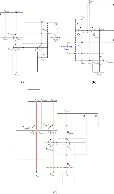
4.1. Matching condition. A sequence(τi)i∈N satisfies thematching condition if, for everyi ∈N, the following conditions hold (see Fig.5):
(i) ifiis of type(B,A), then
τi =τσ (i) ⎛ ⎝1 + a j=1 j k=1 τσ (i)+k
⎞
⎠.
(ii) ifiis of type(A,B), then
τi =τσ (i) ⎛ ⎝1 + a j=1 j k=1 τσ (−1i)−k
⎞
⎠
−1
.
(iii) ifiis of type(A,A), then
τi =τσ (i) ⎛ ⎝1 + a j=1 j k=1 τσ (−1i)−k
⎞ ⎠ −1⎛ ⎝1 + a j=1 j k=1 τσ (i)+k
⎞
(a) (b)
(c)
Fig. 5.The matching condition for theγ-sequence(τγ ,i)i∈N=τ (Gγ, πγ(0,0))with the three possible cases fori∈N. Here we consider the casea=2.aCaseiof type(B,A).bCaseiof type(A,B).cCaseiof type
Fig. 6.The boundary condition for theγ-sequence(τγ ,i)i∈N. Here,J=(K1∪K2)\K0is the right boundary of the Markov rectangleAandIis the unstable spanning leaf segment in the interior ofAsuch thatI∩K0= {x}
Lemma 3.For every(G,z)∈Gγ, the sequenceτ (G,z)satisfies the matching condition.
Proof. Putting together Lemma2 and Eq. (4) in Appendix6, we obtain thatτG,i = σG(Ki : Ki+1), for everyi ∈N. Hence Lemma3follows from Lemma5in Appendix
6. ⊓⊔
We note that every sequence(βi)i∈N\σ (N)determines, uniquely, a sequence(τi)i∈N satisfying the matching condition as follows: (i) for everyi ∈N\σ (N), defineτi =βi
and (ii) for everyi ∈σ (N), inductively ini, defineτσ (i)using the matching condition, i.e.τi, that was previously defined inductively, and elementsτk =βk ∈N\σ (N).
4.2. Boundary condition. A sequence(τi)i∈N satisfies theboundary condition, if the following limits are well-defined and satisfy the conditions:
(i) lim
i→+∞τ −1 Fi+2
1 +τF−1
i+1
=0
(ii) lim
i→+∞τFi
1 +τFi+1
=0
Following the proof of Lemma 3.6 in [21] we get that, for every(G,z) ∈ Gγ, the sequenceτ (G,z)satisfies the boundary condition (see Fig.6).
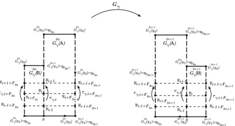
Fig. 7.The sequence(τG,i)i∈Nsatisfies the exponentially fastγ-Fibonacci repetitive property. We observe
that lim
n→∞yFn=y0
C ≥0 and 0< μ <1 such that
τi+Fm −τi
≤Cμm,
for everym≥5 and 3≤i<Fm−1and, also, fori ∈ {1,2}ifmis even.
Following the proof of Lemma 3.7 in [21] we get that, for every(G,z)∈ Gγ, the sequenceτ (G,z)satisfies the exponentially fastγ-Fibonacci repetitive condition (see Fig.7).
4.4. γ-Tilings. Aγ-tilingis a sequence(τi)i∈Nof positive numbers satisfying the expo-nentially fastγ-Fibonacci repetitive condition, the matching condition and the boundary condition. LetTγ be the set of allγ-tilings.
Since, for every(G,z)∈ Gγ, the sequenceτ (G,z)satisfies the exponentially fast
γ-Fibonacci repetitive condition, the boundary condition and the matching condition, we obtain thatτ (G,z)is aγ-tiling.
Theorem 3.The mapτ :Gγ →Tγ determines a one-to-one correspondence between marked smooth conjugacy classes of Anosov diffeomorphisms inGγ andγ-tilings.
The proof of Theorem3follows as the proof of Theorem 1.1 in [21].
Theorem 3 implies the existence of an infinite dimensional space of well-characterizedγ-sequences. However, we are only able to explicit the rigidγ-sequence.
5. Tilings Rigidity
We will give conditions in the regularity of the holonomies of the marked Anosov diffeomorphims such that the corresponding affine tilings are rigid.
LetG ∈ G be aC1+ Anosov diffeomorphism topologically conjugate to Gγ by a homeomorphismh. Recall thatMG =h(Mγ)= {h(A),h(B)}is a Markov partition of G. Let M,N ∈ MG be two Markov rectangles, and let the points x ∈ i nt(M)
a stable leaf segmentℓu(x,y)such that (i) xand yare the endpoints ofℓs(x,y), i.e.
∂ℓs(x,y) = {x,y}, and (ii)ℓs(x,y) ⊂ ℓs(x,M)∪ℓs(y,N). Let P = PM be the
set of all pairs(M,N)with unstable holonomically related points. For every Markov rectangle M ∈ MG, choose a pointx ∈ i nt(M)and consider the unstable spanning leaf segmentℓu(x,M). LetI = {ℓuM : M ∈ M}. For every pair(M,N) ∈ P there exist maximal unstable leaf segments ℓD(M,N) ⊂ ℓuM andℓC(M,N) ⊂ ℓuN such that the unstable holonomyθ(M,N):ℓ(DM,N)→ℓC(M,N)is well-defined. We call such holonomies
θ(M,N):ℓ(DM,N)→ℓC(M,N)theunstable primitive holonomiesassociated to the Markov partitionMG. The complete set of unstable holonomiesHG consists of all unstable
primitive holonomies and their inverses (see [26,28]).
A diffeomorphismθ :I → J is said to beC1+zygmund, where IandJ are unstable leaf segments, ifθisC1and the derivativeθ′satisfies the zygmund condition, i.e. for all pointsx,y∈I,
θ
′(x)
+θ′(y)−2θ′x+y
2
=χθ(|y−x|) ,
where the function χθ is such that χθ(t) → 0 whent → 0. In particular, a C2+β diffeomorphism, withβ >0, is aC1+zygmunddiffeomorphism. The importance of this smooth class follows from the fact that it corresponds to maps that distort cross-ratios of quadruples of points inIby an amount that iso(|I|)(see [20,30]).
Definition 2.A complete set of unstable holonomies HG is C1+zygmund, if all
holonomies θ ∈ HG are C1+zygmund with respect to the unstable lamination atlas
Lu(G, ρ).
Theorem 4(Rigidity). Every(G,z)∈Gγwith a C1+zygmundcomplete system of unsta-ble holonomies determines a rigidγ-tilingτ (Gγ,z)=τγ.
The proof of Theorem4follows as the proof of Theorem 1.3 in [21].
Acknowledgements. We are thankful to Mikhail Lyubich and to the anonymous referee for useful comments and suggestions. We are grateful to David Rand, Dennis Sullivan, Edson Faria, Flávio Ferreira, Alby Fisher, Aldo Portela, and Yunping Jiang for a number very fruitful and useful discussions on this work and for their friendship and encouragement. We thank LIAAD-INESC TEC, USP-UP project, Faculty of Sciences, Uni-versity of Porto and Calouste Gulbenkian Foundation. We acknowledge the financial support received by the ERDF—European Regional Development Fund through the Operational Programme for Competitiveness and Internationalisation—COMPETE 2020 Programme within project “POCI-01-0145-FEDER-006961”, and by National Funds through the FCT—Fundação para a Ciência e a Tecnologia (Portuguese Foundation for Science and Technology) within project UID/EEA/50014/ 2013 and ERDF (European Regional Development Fund) through the COMPETE Program (operational program for competitiveness) and by National Funds through the FCT within Project “Dynamics, optimization and modelling”, with reference PTDC/MAT-NAN/6890/2014. Alberto Pinto also acknowledges the financial support received through the Special Visiting Researcher Pro-gram (Bolsa Pesquisador Visitante Especial—PVE) “Dynamics, Games and Applications” with reference 401068/2014-5 (call: MEC/MCTI/CAPES/CNPQ/FAPS), at IMPA, Brazil. Part of this research was started during a visit by the authors to the IHES and CUNY, and continued at the Isaac Newton Institute, Univer-sity of Warwick, IMPA, MSRI, SUNY at Stony Brook and Institut Henri Poincaré. We thank them for their hospitality.
6. Appendix: Solenoid Functions
unstable ratio functions and so we are only going to characterize the unstable solenoid functions. Since the Anosov diffeomorphisms have an invariant measure absolutely continuous with respect to Lebesgue, by duality the unstable solenoid function will determine the stable solenoid function and vice-versa.
Letsoldenote the set of all ordered pairs(I,J)of unstable spanning leaf segments of the Markov rectangles AandBofGγ such that the intersection ofI andJ consists of a single endpoint. Since the setsolis topologically a finite disjoint union of disjoint intervals, i.e. the disjoint union of a stable spanning leaf segment ofAand a stable span-ning leaf segment ofB, it has a natural topological structure (see Pinto and Rand [22]).
Definition 3.A functionσ :sol→R+is an(unstable) solenoid function, if the
follow-ing conditions hold: (i)σ is Hölder continuous; (ii)σ satisfies the matching condition; and (iii)σ satisfies the boundary condition.
In the next subsections, we define the properties mentioned in the above definition. LetGbe aC1+Anosov diffeomorphism inG. The(unstable) realized solenoid function
σG:sol→R+is well-defined by
σG(I :J)= lim n→∞
|G−n(hG(J)| |G−n(h
G(I))|
(4)
by the control ratio distortion lemma (see [22]).
Theorem 5.The map G→σGdetermines a one-to-one correspondence between C1+
conjugacy classes of Anosov diffeomorphisms G∈Gγ, that have an invariant measure absolutely continuous with respect to Lebesgue, and solenoid functions.
Proof. By Theorem 3.4 in [28] there is a one-to-one correspondence betweenC1+ con-jugacy classes of Anosov diffeomorphisms and pairs of stable and unstable solenoid function. By Theorem 8.17 in [28], an unstable measure ratio function determines a unique dual stable measure function and vice-versa. For Anosov diffeomorphisms, that have an invariant measure absolutely continuous with respect to Lebesgue, the stable and unstable measure ratio functions are dual and by Lemma 8.5 in [28], there is a one-to-one correspondence between stable (resp. unstable) measure ratio functions and stable (resp. unstable) solenoid functions. Since, the stable function is obtained by duality from the unstable function we obtain the result. ⊓⊔
6.1. Hölder continuity of solenoid functions. We define a pseudo-metricdsol : sol×
sol→R+on the setsolas follows: (i) ifI =I′andJ =J′then dsol(I,J) ,I′,J′=0;
(ii) ifI ∩I′= ∅andJ∩J′= ∅then
dsol
(I,J) ,I′,J′=maxdI,I′,dJ,J′;
(iii) otherwise,
dsol(I,J) ,I′,J′=1.
The solenoid functionσ isHölder continuityif, for allt =(I,J)andt′ =(I′,J′)in
sol, the solenoid functionσ satisfies
σ (t)−σ (t′) ≤O
dsolt,t′α,
6.2. Boundary condition. Let(Ii,Ii+1), (Jj,Jj+1)∈ sol, for eachi ∈ {0, . . . ,m}and
each j ∈ {0, . . . ,n}with the following properties: (i)I0= J0, (ii)∪mi=1Ii = ∪nj=1Jj
and (iii)Ii = Ji for somei ∈1, . . . ,m. Then the following two ratios are equal
m
i=1 i
j=1 |Ij| |Ij−1| =
| ∪im=1Ii| |I0| =
| ∪nj=1Jj| |J0| =
n
i=1 i
j=1 |Jj| |Jj−1|.
We observe that the unstable spanning leaf segmentsI1, . . . ,ImandJ1, . . . ,Jnmust be
boundaries of Markov rectangles. Thus, a realized solenoid functionσGmust satisfy the followingboundary conditionfor all such leaf segments:
m
i=1 i
j=1
σGIj−1: Ij= n
i=1 i
j=1
σGJj−1: Jj. (5)
Let K0,K1,K2andK3be the unstable spanning leaf segments as defined in Sect.3.
Recall that,K0is the unstable spanning leaf segment of the right boundary of the Markov
rectangle B; J =(K1∪K2)\K0 is the unstable spanning leaf segment of the right
boundary of the Markov rectangle A; K1is the unstable spanning leaf segment of the
left boundary of the Markov rectangle A;K2is the unstable spanning leaf segment of
the left boundary of the Markov rectangleB; and soK3∩K2=K3∩J= {y2}. Let I
be the unstable spanning leaf segment in the interior of Asuch thatI ∩K0= {x}(see
Fig.8).
Lemma 4.LetσG : sol → R+ be a realized solenoid function. ThenσG satisfies the
boundary condition if the following two conditions hold:
σG(I :K1)(1 +σG(K1: K2))=σG(I :K0)(1 +σG(K0:J)); (6)
and
σG(K3:K2)(1 +σG(K2:K1))=σG(K3:J)(1 +σG(J :K0)). (7)
Proof. The boundary condition (5) corresponds to
|K1| |I|
1 + |K2|
|K1|
=|K1∪K2| |I| =
|K0∪J| |I| =
|K0| |I|
1 + |J|
|K0|
,
and
|K2| |K3|
1 +|K1|
|K2|
= |K1∪K2| |K3| =
|K0∪J| |K3| =
|J| |K3|
1 +|K0|
|J|
.
Fig. 8.The boundary condition for the realized solenoid functionσG
6.3. Matching condition. Let(I,J)∈sol. Suppose that there are pairs
(I0,I1), (I1,I2), . . . , (In−2,In−1)∈sol
such thatGγI =k−1
j=0Ij andGγJ=n−1j=kIj. Then
|GγJ|
|GγI|
=
n−1
j=k|Ij|
k−1
j=0|Ij| =
n−1
j=k
j
i=1|Ii|/|Ii−1|
1 +k−1
j=1
j
i=1|Ii|/|Ii−1| .
Hence, the realized solenoid functionσG must satisfy thematching condition for all such leaf segments (see Fig.5):
σG(I :J)=
n−1 j=k
j
i=1σG(Ii−1:Ii)
1 +k−1 j=1
j
i=1σG(Ii−1: Ii)
. (8)
Lemma 5.LetσG :sol→R+be a realized solenoid function. For a∈N, the matching
condition holds forσGif, for every(K1,K2)∈sol, the following conditions hold: (i) if K1,K2∈ A, then
σG(K1:K2)= a+1
k=1
σG(Ik :Ik+1)
1 +2a+1
j=a+2
j
k=a+2σG(Ik:Ik+1)
1 +a
j=1
j
k=1σG(Ik :Ik+1)
. (9)
(ii) if K1∈ A and K2∈ B, then
σG(K1:K2)= a+1
k=1
σG(Ik :Ik+1)
⎛ ⎝1 + a j=1 j k=1
σG(Ik :Ik+1)
⎞
⎠
−1
(10)
where I1, . . . ,Ia+2 are such that Gγ(K1) = ∪i=1a+1Ii, Gγ(K2) = Ia+2 and (Ii,Ii+1)∈solfor i ∈ {1, . . . ,a+ 1}.
(iii) if K1∈ B and K2∈ A, then
σG(K1:K2)=σG(I1: I2)
⎛ ⎝1 + a+1 j=2 j k=2
σG(Ik :Ik+1)
⎞
⎠ (11)
where I1, . . . ,Ia+2 are such that Gγ(K1) = I1, Gγ(K2) = ∪a+2i=2Ii and (Ii,Ii+1)∈solfor i ∈ {1, . . . ,a+ 1}.
Proof. If(K1,K2)∈solthen(K1,K2)satisfies either condition(i),(i i)or(i i i)above (see Fig.5). Let us check that the formulas (9), (10) and (11) correspond to the matching condition (8) forσG.
(i) IfK1,K2∈ Athen there exists(Ii,Ii+1)∈sol, fori =1, . . . ,2a+ 2, such that
Gγ(K1)=I1∪ · · · ∪Ia+1andGγ(K2)=Ia+2∪ · · · ∪I2a+2. Furthermore,
|Gγ(K2)| |Gγ(K1)|
=
2a+1 i=a+2|Ii|
a+1
i=1|Ii| =
a+1
k=1 |Ik+1|
|Ik|
⎛
⎝
1 +2a+1 j=a+2
j
k=a+2 |Ik+1|
|Ik|
1 +a j=1
j
k=1 |Ik+1|
|Ik| ⎞
⎠.
Hence, equality (9) follows from equality (8).
(ii) IfK1 ∈ AandK2∈ B then there exists(Ii,Ii+1)∈ sol, fori =1, . . . ,a+ 1,
such thatGγ(K1)=I1∪ · · · ∪Ia+1andGγ(K2)=Ia+2. Furthermore,
|Gγ(K2)| |Gγ(K1)| =
|Ia+2|
a+1 i=1|Ii|
= a+1
k=1 |Ik+1|
|Ik|
⎛ ⎝1 + a j=1 j k=1 |Ik+1|
|Ik|
⎞
⎠
−1
.
Hence, equality (10) follows from equality (8).
(iii) IfK1∈ BandK2∈ A, then there exists(Ii,Ii+1)∈sol, fori =1,2, such that
Gγ(K1)=I1andGγ(K2)=I2∪ · · · ∪Ia+2. Furthermore,
|Gγ(K2)| |Gγ(K1)|
=
a+2
i=2|Ii| |I1| =
|I2| |I1|
⎛ ⎝1 + a+1 j=2 j k=2 |Ik+1|
|Ik|
⎞
⎠.
References
1. Almeida, J.P., Pinto, A.A., Rand D.A.: Renormalization of Circle Diffeomorphism Sequences and Markov Sequences, In: Gracio, C., Fournier-Prunaret, D., Ueta, T., Nishio, Y. (eds.) Nonlinear Maps and their Applications, Selected Contributions from the NOMA 2011 International Workshop. Springer proceed-ings in Mathematics and Statistics
2. Anosov, D.V.: Tangent fields of transversal foliations in U-systems. Math. Notes Acad. Sci. USSR2(5), 818–823 (1967)
3. Bedford, T., Fisher, A.M.: Ratio geometry, rigidity and the scenery process for hyperbolic Cantor sets. Ergod. Theory Dyn. Syst.17, 531–564 (1997)
4. Cawley, E.: The Teichmüller space of an Anosov diffeomorphism ofT2. Invent. Math.112, 351– 376 (1993)
5. Coullet, P., Tresser, C.: Itération d’endomorphismes et groupe de renormalisation. J. Phys.C5, 25 (1978) 6. Feigenbaum, M.: The universal metric properties of nonlinear transformations. J. Stat. Phys.21, 669–
706 (1979)
7. Feigenbaum, M.: Quantitative universality for a class of nonlinear transformations. J. Stat. Phys.19, 25– 52 (1978)
8. Fraenkel, A.S.: Systems of numeration. Am. Math. Monthly92(2), 105–114 (1985)
9. Jacobson, M.V., Swiatek, G.: Quasisymmetric conjugacies between unimodal maps. Stony Brook preprint IMS #1991/16, pp. 1–64 (1991)
10. Jiang, Y.: Asymptotic differentiable structure on Cantor set. Commun. Math. Phys. 155(3), 503– 509 (1993)
11. Jiang, Y.: Renormalization and Geometry in One-Dimensional and Complex Dynamics. Advanced Series in Nonlinear Dynamics. Vol. 10, World Scientific Publishing Co. Pte. Ltd., River Edge, NJ (1996) 12. Jiang, Y.: Smooth classification of geometrically finite one-dimensional maps. Trans. Am. Math.
Soc.348(6), 2391–2412 (1996)
13. Jiang, Y.: On rigidity of one-dimensional maps. Contemp. Math. AMS Ser.211, 319–431 (1997) 14. Jiang, Y.: Metric invariants in dynamical systems. J. Dyn. Differ. Equ.17(1), 51–71 (2005)
15. Jiang, Y.: Teichmüller Structures and Dual Geometric Gibbs Type Measure Theory for Continuous Poten-tials, preprint (2008).arXiv:0804.3104v3[math.DS]
16. Jiang, Y., Cui, G., Gardiner, F.: Scaling functions for degree two circle endomorphisms. Contemp. Math. AMS Ser.355, 147–163 (2004)
17. Jiang, Y., Cui, G., Quas, A.: Scaling functions, Gibbs measures, and Teichmüller space of circle endo-morphisms. Discr. Contin. Dyn. Syst.5(3), 535–552 (1999)
18. Lanford, O.: Renormalization Group Methods for Critical Circle Mappings with General Rotation Num-ber, VIIIth International Congress on Mathematical Physics (Marseille, 1986). pp. 532–536. World Sci-entific Publishing, Singapore (1987)
19. Mañé, R.: Ergodic Theory and Differentiable Dynamics. Springer, Berlin (1987)
20. de Melo, W., van Strien, S.: One-dimensional Dynamics. A series of Modern Surveys in Mathe-maics. Springer, New York (1993)
21. Pinto, A.A., Almeida, J.P., Portela, A.: Golden tilings. Trans. Am. Math. Soc.364, 2261–2280 (2012) 22. Pinto, A.A., Rand, D.A. : Solenoid functions for hyperbolic sets on surfaces. In: Hasselblat, B. (ed.)
Dynamics, Ergodic Theory and Geometry: Dedicated to Anatole Katok, pp. 145–178. MSRI Publica-tions, (2007)
23. Pinto, A.A., Rand, D.A.: Geometric measures for hyperbolic sets on surfaces. Stony Brook preprint IMS #2006/3, pp. 1–54 (2006)
24. Pinto, A.A., Rand, D.A.: Rigidity of hyperbolic sets on surfaces. J. Lond. Math. Soc.71(2), 481– 502 (2004)
25. Pinto, A.A., Rand, D.A.: Smoothness of holonomies for codimension 1 hyperbolic dynamics. Bull. Lond. Math. Soc.34, 341–352 (2002)
26. Pinto, A.A., Rand, D.A.: Teichmüller spaces and HR structures for hyperbolic surface dynamics. Ergod. Theory Dyn. Syst.22, 1905–1931 (2002)
27. Pinto, A.A., Rand, D.A.: ClassifyingC1+structures on dynamic fractals: 1 the moduli space for solenoid functions for Markov maps on train-tracks. Ergod. Theory Dyn. Syst.15, 697–734 (1995)
28. Pinto, A.A., Rand, D.A., Ferreira, F.: Fine Structures of Hyperbolic Diffeomorphisms. Springer Mono-graphs in Mathematics. Springer, Berlin, Heidelberg (2009)
29. Pinto, A.A., Rand, D. A., Ferreira, F.: Cantor exchange systems and renormalization. J. Differ. Eq.273(2), 593–616 (2007)
30. Pinto, A.A., Sullivan, D.: The circle and the solenoid. Dedicated to Anatole Katok On the Occasion of his 60th Birthday. DCDS-A16(2), 463–504 (2006)
32. Schub, M.: Global Stability of Dynamical Systems. Springer, New York (1987)
33. Sullivan, D.: Differentiable structures on fractal-like sets determined by intrinsic scaling functions on dual Cantor sets. In: Proceedings of Symposia in Pure Mathematics, vol. 48, American Mathematical Society (1988)
34. Veech, W.: Gauss measures for transformations on the space of interval exchange maps. Ann. Math. 2115(2), 201–242 (1982)
35. Williams, R.F.: Expanding attractors. Publ. IHES43, 169–203 (1974)
![Fig. 3. The map π S (w) = i S ◦π γ (w, 0)|[−γ , 1], for every w ∈ [−γ , 1], and the points z i = i S (y i ) = π S (w i ), for i ∈ N](https://thumb-eu.123doks.com/thumbv2/123dok_br/16984947.763217/7.659.121.547.78.439/fig-map-π-s-s-π-γ-points.webp)