Volume 364, Number 5, May 2012, Pages 2261–2280 S 0002-9947(2011)05293-1
Article electronically published on December 16, 2011
GOLDEN TILINGS
A. A. PINTO, J. P. ALMEIDA, AND A. PORTELA
Abstract. We introduce the notion of golden tilings, and we prove a one-to-one correspondence between (i) smooth conjugacy classes of Anosov dif-feomorphisms, with an invariant measure absolutely continuous with respect to the Lebesgue measure, (ii) affine classes of golden tilings and (iii) solenoid functions. The solenoid functions give a parametrization of the infinite di-mensional space consisting of the mathematical objects described in the above equivalences.
1. Introduction
Inspired in the works of Y. Jiang [12], A. Pinto and D. Sullivan [28] and A. Pinto and D. Rand [19], we introduce the notion of golden tilings. The golden tilings record the infinitesimal geometric structure determined by the dynamics along the unstable leaf that is invariant by the Anosov diffeomorphism. We define the proper-ties of the golden tilings using the Fibonacci decomposition of the natural numbers instead of the dyadic decomposition, because the Fibonacci decomposition has the advantage of encoding, in a natural way, the combinatorics determined by the Markov partition along the unstable leaf. Our goal is to exhibit a natural corre-spondence between golden tilings, Anosov diffeomorphisms and solenoid functions.
1.1. Main theorem. Let γ = 2/(1 +√5) be the inverse of the golden number. The(golden) Anosov automorphism GA: T→Tis given byGA(x, y) = (x+y, x), where T is equal to R2/(vZ×wZ) with v = (γ,1) and w = (−1, γ). A C1+ (golden) Anosov diffeomorphismG: T→Tis aC1+αdiffeomorphism, withα >0, such that (i) G is topologically conjugate to GA by a map hG; (ii) the tangent bundle has a C1+α uniformly hyperbolic splitting into a stable direction and an unstable direction (see [30]). We denote by G the set of all such C1+ Anosov
diffeomorphisms with an invariant measure absolutely continuous with respect to the Lebesgue measure.
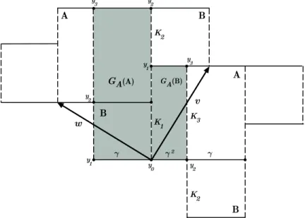
The eigenvalues of the Anosov automorphism GA areμ− =−γ andμ+ = 1/γ. Let π : R2 → T be the natural projection of R2 in T. Let A0 and B0 be the
rectangles [0,1]×[0,1] and [−γ,0]×[0, γ], respectively (see Figure 1). A Markov partitionMAofGAis given byA=π(A0) andB=π(B0). The unstable manifolds
ofGA correspond to the projection byπof the vertical lines of the plane, and the stable manifolds ofGA are the projection byπof the horizontal lines of the plane. LetW0be the positive vertical axis ofR2. HenceW =π(W0) is the unstable leaf of GAwith only one endpointy0=π(0,0) that is the fixed point ofGA. The unstable
Received by the editors February 21, 2008 and, in revised form, January 5, 2010. 2000Mathematics Subject Classification. Primary 37C15; Secondary 37C40.
Key words and phrases. Anosov diffeomorphisms, circle diffeomorphisms, dynamics, renormal-ization, solenoid functions, tilings.
c
2011 American Mathematical Society
leafW passes first through all the unstable boundaries of the Markov rectanglesA
and B. Let the unstable spanning leaf segmentK1 be the left unstable boundary of the Markov rectangleA(see the definition of a spanning leaf segment in Section 2.1). Let the unstable spanning leaf segment K2 be the left unstable boundary of the Markov rectangle B. Let K3, K4, . . . ∈ W be the unstable leaf segments defined, inductively, as follows: (i) Ki is an unstable spanning leaf of a Markov rectangle, for every i ≥3; (ii)Ki∩Ki+1 ={yi} is a common boundary point of bothKi andKi+1, for everyi≥2 (see Figure 1). We note thatW =i≥1Ki.
Figure 1. The golden automorphismGA.
Theorem 1.1 (Flexibility). There is a well-defined map G → (aG
i )i∈N that
as-sociates to each C1+ Anosov diffeomorphism G in G the golden sequence (aG i )i∈N
given by
aG
i = nlim→∞|
G−n(h
G(Ki+1))|
|G−n(h G(Ki))|
,
where|I|means the length of the unstable leaf segmentIwith respect to a Riemann-ian metric on T. Furthermore, this map determines a one-to-one correspondence
between smooth conjugacy classes of Anosov diffeomorphisms in G and golden se-quences.
We leave the definition of the golden sequences to Section 3.7, and we will prove Theorem 1.1 in Section 3.8.
The Fibonacci numbers F1, F2, F3, . . . are inductively given by the well-known relationFn+2 =Fn+1+Fn, withn≥1, where we chooseF1= 1 andF2= 2. For any natural numberi∈N, we define the finite sequenceFn
0, Fn1, . . . , Fnpas follows: (i)Fn0is the largest Fibonacci less or equal toi; (ii) inductively, ifFn0+· · ·+Fnk−1<
i, then Fnk is the largest Fibonacci less than or equal toi−
Fn0+· · ·+Fnk−1
. We observe that there is an integerp∈Nand a Fibonacci number Fn
p such that
We callFn0, . . . , Fnp theFibonacci decomposition ofi∈N. We observe that every natural numberi∈Nhas a unique Fibonacci decomposition.
Definition 1.2. Therigid golden sequence (aR
i )i∈Nis defined as follows. For every
i∈N, with Fibonacci decompositionFn
0, . . . , Fnp, we define (i) aR
i =γ−1if either (np= 1 andnp−1 is odd) or (np= 2 andnp−1is even);
(ii) aR
i =γif either (np= 1 andnp−1 is even) or (np>2 andnp is odd); (iii) aR
i = 1 if either (np= 2 andnp−1is odd) or (np>2 andnp is even). In Theorem 1.1, we prove the existence of an infinite dimensional space of well-characterized golden sequences. However, the only golden sequence that we are able to make explicit is the rigid golden sequence.
Theorem 1.3(Rigidity).Every Anosov diffeomorphismG∈ G, with aC1+zygmund
complete system of unstable holonomies, determines a golden sequence(aG
i )i∈Nthat
is rigid.
The definition of aC1+zygmund complete system of unstable holonomies and the proof of Theorem 1.3 are given in Section 4.
2. Solenoid functions
LetGbe aC1+Anosov diffeomorphisminG. We define the mapG
ι=Gifι=u or Gι = G−1 if ι=s. For ι ∈ {s, u} and x∈ T, we denote the localι-manifolds through xby
Wι(x, ε) =
y∈T:d(G−n
ι (x), G−ιn(y))≤ε, for alln≥0
,
where dis the distance determined by a Riemannian metric on the torus. By the Stable Manifold Theorem [30], these sets are respectively contained in the stable and unstable immersed manifolds
Wι(x) =
n≥0 Gn
ι
Wι
G−n ι (x), ε0
which are the image ofC1+αimmersionsκ
ι,x:R→T, for some 0< α≤1 and some smallε0>0. Anopen(resp. closed)ι-leaf segmentIis defined as a subset ofWι(x) of the formκι,x(I1), whereI1 is an open (resp. closed) subinterval (non-empty) in R. Anι-leaf segmentis either an open or closed ι-leaf segment. The endpoints of an ι-leaf segment I = κι,x(I1) are the points κι,x(u) and κι,x(v), where u and v are the endpoints ofI1. Theinterior of an ι-leaf segment I is the complement of its boundary. A map c : I → R is anι-leaf chart of anι-leaf segment I ifc is a homeomorphism onto its image.
2.1. Spanning leaf segments. One can find a small enoughǫ0>0 such that for every 0< ǫ < ǫ0there isδ=δ(ǫ)>0 with the property that, for all pointsw, z∈T withd(w, z)< δ,Wu(w, ǫ) andWs(z, ǫ) intersect in a unique point that we denote by
[z, w] =Wu(w, ǫ)
∩Ws(z, ǫ).
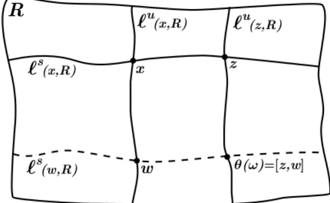
a rectangle R, for eachx ∈R there are closed unstable and stable leaf segments of T, ℓu(x, R) ⊂Wu(x) andℓs(x, R) ⊂Ws(x) such that R = [ℓu(x, R), ℓs(x, R)]. The leaf segmentsℓu(x, R) andℓs(x, R) are called, respectively,unstableandstable
spanning leaf segments (see Figure 2).
Figure 2. A basic unstable holonomyθ:ℓu(x, R)→ℓu(z, R).
2.2. Basic holonomies. Suppose thatxandzare two points inside any rectangle
R of T. Let ℓu(x, R) and ℓu(z, R) be two unstable spanning leaf segments of R containing, respectively, xand z. We define the map θ : ℓu(x, R) → ℓu(z, R) by
θ(w) = [z, w] (see Figure 2). Such maps are called the basic unstable holonomies. They generate the pseudo-group of all unstable holonomies. Similarly, we can define thebasic stable holonomies.
2.3. Lamination atlas. Theunstable lamination atlasL=Lu(G, ρ), determined
by a Riemannian metricρ, is the set of all mapse:I→R, where eis an isometry between the induced Riemannian metric on the unstable leaf segment I and the Euclidean metric on the reals. We call the maps e ∈ L the unstable lamination charts. By Theorem 2.1 in [23], the basic unstable and stable holonomies areC1+
with respect to the lamination atlasL(see also [1] and [17]).
2.4. HR structures. TheHR structureassociates an affine structure to each sta-ble and unstasta-ble leaf segment ofGAin such a way that these vary H¨older continu-ously with the leaf and are invariant underGA (see [24]).
An affine structure on a stable or unstable leaf of GA is equivalent to a ratio
function r(I:J) which can be thought of as prescribing the ratio of the size of two leaf segmentsIandJ in the same stable or unstable leaf. Aratio functionr(I:J) is positive (we recall that each leaf segment has at least two distinct points) and continuous in the endpoints ofI andJ. Moreover,
(2.1) r(I:J) =r(J :I)−1andr(I1∪I2:K) =r(I1:K) +r(I2:K),
providedI1 andI2 intersect in at most one of their endpoints.
We say thatris anunstable ratio function if (i) for all unstable leaf segmentsK
a rectangleR, and for every unstable leaf segment I0 ⊂I and every unstable leaf segmentI1⊂I,
(2.2)
logr(θI0:θI1)
r(I0:I1)
≤ O
((d(I, J))ǫ),
whereǫ∈(0,1) depends uponR and the constant of proportionality also depends uponR, but not on the segments considered. Sincer satisfies condition (2.2) and defines an affine structure on each leaf that is invariant under GA, we say that r is a tranversely H¨older unstable ratio function. An HR-structure is a pair (rs, ru) consisting of a stable and an unstable ratio function.
2.5. Realized HR structures. LetGbe aC1+Anosov diffeomorphism in
G, and letLu(G, ρ) be an unstable lamination atlas associated to a Riemannian metricρ. If I is an unstable leaf segment, then by |I| we mean the length of the unstable leaf containingI measured using the Riemannian metricρ. LethG:T→Tbe the topological conjugacy between the automorphism GA and the Anosov diffeomor-phism G. Using the mean value theorem and the fact that G is C1+α uniformly hyperbolic, for some α >0, for all short unstable leaf segments K of GA and all leaf segmentsIandJ contained inK, the unstable realized ratio functionru
G given by
ru
G(I:J) = nlim→∞|
G−n(h G(J))|
|G−n(h G(I))| (2.3)
is well defined (see Lemma 3.6 in [24]). Similarly, we have the definition of the stable realized ratio functionrs
G.
Lemma 2.1. The map G→ ru
G determines a one-to-one correspondence between
C1+ conjugacy classes of Anosov diffeomorphismsGin
G and unstable ratio func-tions.
Proof. By Theorem 5.1 in [24], there is a one-to-one correspondenceG→(rs G, rGu) between C1+ conjugacy classes of Anosov diffeomorphisms G and HR-structures
(rs
G, ruG). By Lemma 5 in [19], the unstable ratio functionrGu determines, uniquely, the stable ratio functionrs
G if the Anosov diffeomorphismGhas an invariant mea-sure that is absolutely continuous with respect to the Lebesgue meamea-sure (see also
[3]).
2.6. Realizable solenoid functions. Let soldenote the set of all ordered pairs (I, J) of unstable spanning leaf segments of the Markov rectangles A and B of
GA such that the intersection of I and J consists of a single endpoint. Since the set solis topologically a finite disjoint union of disjoint intervals, i.e. the disjoint union of a primary stable leaf ofAand a primary stable leaf ofB, it has a natural topological structure.
We define a pseudo-metricdsol:sol×sol→R+ on the setsolby
dsol((I, J),(I′, J′)) = max{d(I, I′), d(J, J′)} .
LetGbe aC1+Anosov diffeomorphism in
G. We refer to the restrictionru
G|solof an unstable ratio functionru
2.7. H¨older continuity of solenoid functions. The H¨older continuity of sole-noid functions means that for allt= (I, J) andt′= (I′, J′) in sol,
|σG(t)−σG(t′)| ≤ O(dsol(t, t′))α,
for someα >0.
2.8. Matching condition. Let (I, J)∈sol. Suppose that there are pairs (I0, I1),(I1, I2), . . . ,(In−2, In−1)∈sol
such thatGAI=kj=0−1Ij andGAJ =nj=−k1Ij. Then
|GAJ|
|GAI| =
n−1
j=k |Ij| k−1
j=0|Ij| =
n−1
j=k
j
i=1|Ii|/|Ii−1|
1 + kj=1−1j
i=1|Ii|/|Ii−1| .
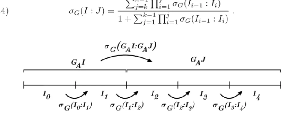
Hence, the realized solenoid functionσG must satisfy the matching condition (see Figure 3) for all such leaf segments:
(2.4) σG(I:J) =
n−1
j=k
j
i=1σG(Ii−1:Ii) 1 + kj=1−1j
i=1σG(Ii−1:Ii)
.
Figure 3. The matching condition for the solenoid function σG withk= 2 andn= 5.
Lemma 2.2. Let σG : sol → R+ be a realized solenoid function. The matching
condition holds forσG if, for every (K1, K2)∈sol, the following conditions hold:
(i) IfK1, K2∈A, then
(2.5) σG(K1:K2) =
σG(I1:I2)σG(I2:I3) (1 +σG(I3:I4)) 1 +σG(I1:I2)
,
where I1, I2, I3 and I4 are such that GA(K1) =I1∪I2, GA(K2) =I3∪I4
and(Ii, Ii+1)∈solfori∈ {1,2,3}. (ii) If K1∈A andK2∈B, then
(2.6) σG(K1:K2) =
σG(I1:I2)σG(I2:I3) 1 +σG(I1:I2)
,
where I1, I2 and I3 are such that GA(K1) = I1∪I2, GA(K2) = I3 and (Ii, Ii+1)∈solfori∈ {1,2}.
(iii) IfK1∈B andK2∈A, then
(2.7) σG(K1:K2) =σG(I1:I2) (1 +σG(I2:I3)),
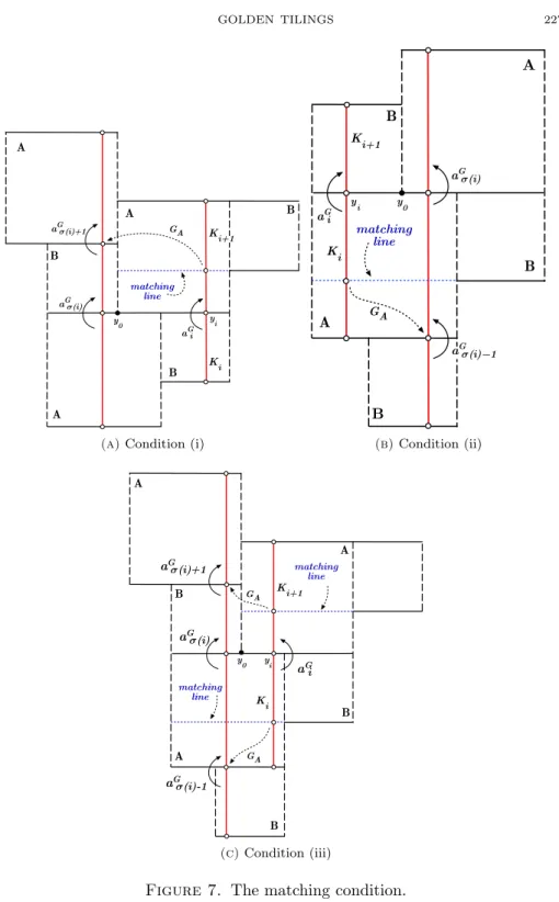
Proof. If (K1, K2) ∈ sol, then (K1, K2) satisfies either condition (i), (ii) or (iii) above (see Figure 7). Let us check that the formulas (2.5), (2.6) and (2.7) corre-spond to the matching condition (2.4) forσG:
(i) If K1, K2 ∈ A, then there exists (Ii, Ii+1)∈sol, fori = 1,2,3, such that GA(K1) =I1∪I2 andGA(K2) =I3∪I4. Furthermore,
|GA(K2)|
|GA(K1)|
= |I3|+|I4| |I1|+|I2| =
|I2|
|I1|
|I3|
|I2|
1 +|I4| |I3| 1 +
|I2|
|I1| −1
.
Hence, equality (2.5) follows from equality (2.4).
(ii) IfK1∈AandK2∈B, then there exists (Ii, Ii+1)∈sol, fori= 1,2, such
thatGA(K1) =I1∪I2 andGA(K2) =I3∪I4. Furthermore,
|GA(K2)|
|GA(K1)|
= |I3| |I1|+|I2| =
|I2| |I1|
|I3| |I2|
1 + |I2| |I1|
−1 .
Hence, equality (2.6) follows from equality (2.4).
(iii) IfK1∈BandK2∈A, then there exists (Ii, Ii+1)∈sol, fori= 1,2, such
thatGA(K1) =I1 andGA(K2) =I2∪I3. Furthermore,
|GA(K2)|
|GA(K1)|
= |I2|+|I3| |I1| =
|I2|
|I1|
1 +|I3| |I2|
.
Hence, equality (2.7) follows from equality (2.4).
2.9. Boundary condition. Let (Ii, Ii+1),(Jj, Jj+1)∈sol, for eachi∈ {0, . . . , m}
and eachj ∈ {0, . . . , n} with the following properties: (i)I0 =J0, (ii) m
i=1Ii =
m
j=1Jj and (iii) Ii=Jj for alli≥1 and allj ≥1. Then the following two ratios are equal: m i=1 i j=1
|Ij|
|Ij−1|
= |
m
i=1Ii|
|I0| =
|n
i=1Jj|
|J0| =
n i=1 i j=1
|Jj|
|Jj−1| .
We observe that the unstable spanning leaf segmentsI1, . . . , ImandJ1, . . . , Jnmust be boundaries of Markov rectangles. Thus, a realized solenoid function σG must satisfy the following boundary condition for all such leaf segments:
(2.8) m i=1 i j=1
σG(Ij−1:Ij) = n i=1 i j=1
σG(Jj−1:Jj) .
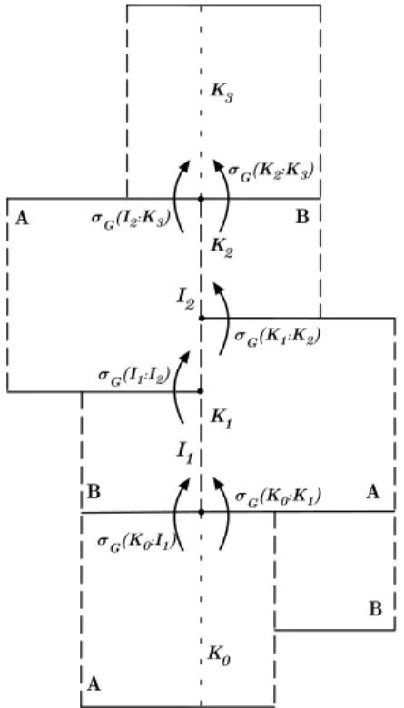
LetK1,K2andK3be the unstable spanning leaf segments as defined in Section 1.1. LetK0be the unstable spanning leaf segment inAsuch thatK0∩K1={y0}. Let the unstable spanning leaf segment I1 be the right boundary of the Markov rectangle B and let the unstable spanning leaf segment I2 be the right boundary of the Markov rectangleA(see Figure 4).
Lemma 2.3. Let σG : sol → R+ be a realized solenoid function. The boundary
condition holds forσG if the following conditions hold:
(2.9) σG(K0:K1)(1 +σG(K1:K2)) =σG(K0:I1)(1 +σG(I1:I2))
and
Proof. Since I1 and K2 are the unstable boundaries of the Markov rectangle B
and I2 and K1 are the unstable boundaries of the Markov rectangle A, then the boundary condition (2.8) corresponds to
|K1|
|K0|
1 +|K2| |K1|
= |K1∪K2| |K0| =
|I1∪I2|
|K0| =
|I1|
|K0|
1 +|I2| |I1|
and
|K2|
|K3|
1 +|K1| |K2|
=|K1∪K2| |K3| =
|I1∪I2|
|K3| = |I2|
|K3|
1 +|I1| |I2|
.
Hence, the boundary condition forσG is given by (2.9) and (2.10).
Figure 4. The boundary condition for the realized solenoid functionσG.
2.9.1. Solenoid functions.
Definition 2.4. A functionσ:sol→R+ is an(unstable) solenoid function if the following conditions hold: (i) σ is H¨older continuous; (ii)σ satisfies the matching condition given by the equalities (2.5), (2.6) and (2.7); and (iii) σ satisfies the boundary condition given by the equalities (2.9) and (2.10).
By Theorem 6.1 in [24], we have the following equivalence:
Lemma 2.5. The map r→r|solgives a one-to-one correspondence between ratio functions and solenoid functions.
Corollary 2.6. The map G → rG|sol determines a one-to-one correspondence
between C1+ conjugacy classes of Anosov diffeomorphisms G in G and solenoid functions rG|solin SOL.
3. Golden tilings
Recall from Section 1.1 the definitions of the unstable leaf segmentsK1, K2, . . . ,
and the unstable leafW =
i≥1Ki. By construction, the set
L={(Ki, Ki+1), i∈N}
is contained insoland is dense in sol. 3.1. Realized golden sequences.
Lemma 3.1. There is a well-defined map G → (aG
i )i∈N that associates to each
C1+ Anosov diffeomorphism Gin
G the sequence (aG
i )i∈Ngiven by
aG
i = lim
n→∞
|G−n(h
G(Ki+1))|
|G−n(h G(Ki))|
.
Furthermore, aG
i =σG(Ki:Ki+1).
Recall thathG is the topological conjugacy betweenGand the Anosov automor-phismGA.
Proof. By Lemma 2.5 and equation (2.3) we get that σG(Ki : Ki+1) = ruG(Ki :
Ki+1), where
ru
G(Ki:Ki+1) = lim
n→∞
|G−n(h
G(Ki+1))|
|G−n(h G(Ki))| is well defined. Since, by construction,aG
i =rGu(Ki:Ki+1), we get that aGi is well defined andaG
i =σG(Ki:Ki+1).
3.2. Fibonacci marking of the unstable leaf.
Lemma 3.2. For every i∈ Nwith Fibonacci decomposition Fn
0, . . . , Fnp the
fol-lowing conditions hold:
(i) Ki∈B and Ki+1 ∈A if either (np = 1 andnp−1 is odd) or (np = 2and
np−1 is even);
(ii) Ki∈A andKi+1∈B if either (np= 1 andnp−1 is even) or (np>2 and
np is odd);
(iii) Ki, Ki+1 ∈ A if either (np = 2 and np−1 is odd) or (np > 2 and np is
even).
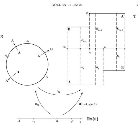
Proof. Letπ :R2 →T be the natural projection, whereT=R2/(vZ×wZ). Let S = R/[1 +γ]Z be the clockwise oriented circle with the metric induced by the Euclidean metric onR. Let πS :R→S be the natural projection. The projection
πShas the property that
πS(x) =πS(x+ 1 +γ),
for everyx∈R. Let iS:S→Tbe the natural inclusion. The inclusioniShas the property that
π(x,0) =iS◦πS(x),
for every x∈ R. Recall that K0 is the unstable spanning leaf segment such that
leaf segments such thatW =
i≥1Ki (see Section 1.1). For every i∈N0, (i) let yi ∈Tbe the point given by {yi}=Ki∩Ki+1; (ii) let zi =i−S1(yi); and (iii) let
wi∈[−1, γ] be such thatπS(wi) =zi. Hence, for everyi∈N0 (see Figure 5),
(i) ifwi∈(−γ,0), then Ki∈AandKi+1∈B;
(ii) ifwi∈(0, γ2), thenKi, Ki+1∈A;
(iii) if wi∈[−1,−γ)∪(γ2, γ], then Ki ∈BandKi+1∈A.
Letg:S→Sbe the golden rigid rotation with rotation numberγ. The mapghas the property that
g◦πS(x) =πS(x+ 1),
for every x∈R. Since GA : T→ Tis an Anosov automorphism, we obtain that
g(zi) = zi+1, for every i ∈ N0. Let us denote by ℓ(y0, yi) the leaf segment with endpoints y0 and yi. Since GA : T → T is the golden Anosov automorphism, if the leaf ℓ(y0, yi) contains mA spanning leaf segments of the Markov rectangle A and mB spanning leaf segments of the Markov rectangle B, then GA(ℓ(y0, yi)) =
ℓ(y0, GA(yi)) containsmA+mB spanning leaf segments of the Markov rectangleA andmAspanning leaf segments of the Markov rectangleB. Hence, by induction, we have thatGA(yFi) =yFi+1, whereF1, F2, . . .are the Fibonacci numbers. Thus, for everyi∈N, we have thatGi−1
A (y1) =yFi, and sod(y0, yFi) =γ
i andπ((
−γ)i,0) =
yFi. Thusg
Fi(z0) =z
Fi =πS((−γ)
i). Sinceg is the golden rigid rotation, we have that
(3.1) gFi(π
S(x)) =πS(x+ (−γ)i),
for everyx∈R andi∈N. Hence, for everyi ∈Nwith Fibonacci decomposition
Fn0, . . . , Fnp, we obtain
zi=gi(z0) =gFn0+···+Fnp(z0).
Thus, by equality (3.1), we have that
gFn0+···+Fnp(z0) =π S
p
i=0
(−γ)ni
.
Noting that +i=0∞γ2i = (1−γ2)−1=γ−1, we obtain
p
i=0
(−γ)ni <
j≥0
γ2+2j=γ
and
p
i=0
(−γ)ni >
j≥0
−γ1+2j=−1.
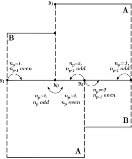
Therefore, taking wi = pj=0(−γ)nj ∈[−1, γ] we obtain thatπS(wi) =zi. Now, there are six distinct cases to consider depending upon the Fibonacci decomposition
Fn0, . . . , Fnp ofi(see Figure 6):
(i) if np = 1 and np−1 is odd, then wi ∈ [−1,−γ), and so Ki ∈ B and
Ki+1∈A;
(ii) if np = 1 and np−1 is even, then wi ∈ (−γ,−γ2), and so Ki ∈ A and
Ki+1∈B;
(iii) if np= 2 andnp−1 is odd, thenwi∈(γ3, γ2), and soKi, Ki+1∈A;
Figure 5. The mapiS◦πS.
(v) ifnp>2 andnp is odd, thenwi∈(−γ2,0), and soKi∈AandKi+1 ∈B;
(vi) ifnp>2 andnp is even, thenwi∈(0, γ3), and so Ki, Ki+1∈A.
3.3. Fibonacci shift. We define the Fibonacci shift σ : N → N as follows. For everyi ∈ N, let Fn
0, . . . , Fnp be the Fibonacci decomposition associated to i, i.e.
i = Fn0+· · ·+Fnp. If np = 1, then we define σ(i) = Fn0+1+· · ·+Fnp+1. If
np = 1 and np−1 is odd, then we define σ(i) = Fn0+1+· · ·+Fnp−1+1+F1. If
np = 1 and np−1 is even, then we define σ(i) = Fn0+1 +· · ·+Fnp−1+1 +F2. Hence, the inverse of the Fibonacci shift σ−1(i) is given as follows: if n
p = 1, then σ−1(i) = F
n0−1+· · ·+Fnp−1; if np = 1 and np−1 is even, then σ
−1(i) = Fn0−1+· · ·+Fnp−1−1+F1; ifnp= 1 andnp−1is odd, thenσ
−1(i) =∅.
Remark 3.3. We observe that for Fnp = F1 the definition of the Fibonacci shift is somewhat unnatural. This is due to the fact that we consider, for simplicity, the Fibonacci sequenceF1= 1, F2= 2, F3= 3, F4= 5, . . . instead of the sequence
F0 = 1, F1 = 1, F2 = 2, F3 = 3, F4 = 5, . . .. If we consider the sequence F0 = 1, F1 = 1, F2 = 2, F3 = 3, F4 = 5, . . ., then we have to change the Fibonacci decomposition of the numberi accordingly with the following rule: ifnp−1 is odd
and i−(Fn0 +· · ·+Fnp−1) = 1, then np = 0. In this case, for every i ∈ N, we define σ(i) = Fn0+1+· · ·+Fnp−1+1+Fnp+1. We get that if np = 0, then
σ−1(i) =F
n0−1+· · ·+Fnp−1, and if np= 0, thenσ
−1(i) =
Figure 6. The location of the point yi depending upon the Fi-bonacci decomposition ofi.
3.4. Matching condition. We say that a sequence (ai)i∈Nsatisfies thematching
condition if, for everyi=Fn0+· · ·+Fnp, the following conditions hold: (i) If either (np= 1 andnp−1 is odd) or (np= 2 andnp−1 is even), then
aσ(i)=aiaσ(i)+1+ 1
−1 .
(ii) If either (np= 1 andnp−1 is even) or (np>2 and np is odd), then
aσ(i)=ai
a−σ(1i)−1+ 1.
(iii) If either (np= 2 andnp−1 odd) or (np>2 andnp is even), then
aσ(i)=
ai1 +aσ(i)−1 aσ(i)−11 +aσ(i)+1
.
Lemma 3.4. The sequence(aG
i )i∈N satisfies the matching condition.
Proof. By Lemma 3.1, we have that aG
i =σG(Ki :Ki+1), for every i∈N. Hence
Lemma 3.4 follows from putting together Lemma 2.2 and Lemma 3.2.
(a)Condition (i) (b)Condition (ii)
(c)Condition (iii)
Figure 7. The matching condition.
aj of the sequence with
Figure 8. The boundary condition.
3.5. Boundary condition. A sequence (ai)i∈Nsatisfies theboundary condition if the following limits are well defined and satisfy the inequalities:
(i) lim i→+∞a
−1
Fi+2
1 +a−Fi1+1
= 0.
(ii) lim
i→+∞aFi(1 +aFi+1)= 0.
Lemma 3.6. The sequence(aG
i )i∈N satisfies the boundary condition.
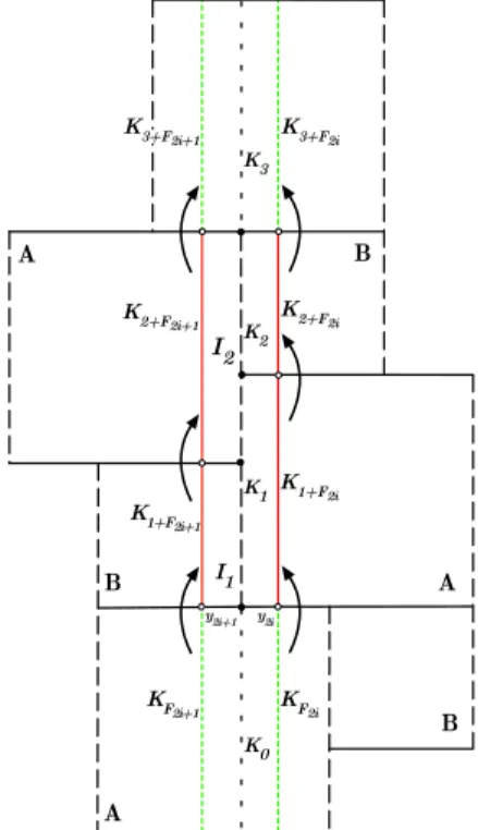
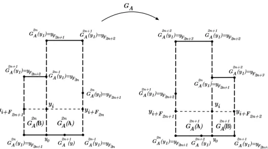
Proof. We observe thatd(KFn, K0) =γ
n,d(K
F2n+1+1, I1) =γ
2n+1,d(K
F2n+1+2, I2) =γ2n+1,d(K
F2n+1, K1) =γ
2n,d(K
F2n+2, K2) =γ
2n and d(K
Fn+3, K3) =γ
n (see
Figure 8). By continuity ofσa, we have that
lim n→∞a
G
F2n(1 +a
G F2n+1)
= lim
n→∞σG(KF2n:KF2n+1)(1 +σG(KF2n+1:KF2n+2))
=σG(K0:K1)(1 +σG(K1:K2))
and
lim n→∞a
G
F2n+1(1 +a G F2n+1+1)
= lim
Hence, by equality (2.9), we obtain that the golden sequence (aG
i )i∈N satisfies the boundary condition (i). By continuity ofσG, we have that
lim n→∞(a
G F2n+2)
−1(1 + (aG F2n+1)
−1)
= lim
n→∞σG(KF2n+3:KF2n+2)(1 +σG(KF2n+2:KF2n+1))
=σG(K3:K2)(1 +σG(K2:K1)) and
lim n→∞(a
G F2n+1+2)
−1(1 + (aG F2n+1+1)
−1)
= lim
n→∞σG(KF2n+1+3:KF2n+1+2)(1 +σG(KF2n+1+2:KF2n+1+1)) =σG(K3:I2)(1 +σG(I2:I1)).
Hence, by equality (2.10) we obtain that the golden sequence (aG
i )i∈Nsatisfies the
boundary condition (ii).
3.6. The exponentially fast Fibonacci repetitive property. A sequence (ai)i∈Nis said to beexponentially fast Fibonacci repetitive if there exist constants
C≥0 and 0< μ <1 such that
|ai+Fm−ai| ≤Cμ
m,
for everym≥5 and 3≤i < Fm−1 and, also, fori∈ {1,2} ifm is even.
Lemma 3.7. The sequence(aG
i )satisfies the exponentially fast Fibonacci repetitive
property.
Proof. For everym≥5, we have that eitherm= 2norm= 2n+ 1 for somen≥2 (see Figure 9). Recall thatKi∩Ki+1={yi}, for everyi∈N0.
(i) Case m= 2n. For 1≤i < F2n−1, the unstable spanning leaf segmentsKi,
Ki+1,Ki+F2n andKi+1+F2n belong toG
2n(A). Hence, we obtain that
d(Ki, Ki+F2n)≤C0|yi−yi+F2n| ≤C0γ
2n,
for some C0 ≥1 and 0 < γ < 1. By H¨older continuity of the solenoid function, there exist constantsC≥1 and α <1 such that
|aGi −aGi+F2n| = |σG(Ki:Ki+1)−σG(Ki+F2n:Ki+1+F2n)|
< C γ2nα
= C(γα)2n.
(ii) Casem= 2n+ 1. For 3≤i < F2n, the unstable spanning leaf segmentsKi,
Ki+1,Ki+F2n+1 andKi+1+F2n+1 belong toG
2n(B). Hence, we obtain that
d(Ki, Ki+F2n+1)≤C0|yi−yi+F2n+1| ≤C0γ
2n+1,
for some C0 ≥1 and 0 < γ < 1. By H¨older continuity of the solenoid function, there exist constantsC≥1 and α <1 such that
|aG
i −aGi+F2n+1| = |σG(Ki:Ki+1)−σG(Ki+F2n+1 :Ki+1+F2n+1)|
< C
γ2n+1α
= Cγα(γα)2n.
Hence, the sequence (aG
i ) satisfies the exponentially fast Fibonacci repetitive
Figure 9. The exponentially fast Fibonacci repetitive condition.
3.7. Golden tilings. A tiling T ={Ii⊂R : i∈N} of the positive real line is a collection of tiling intervalsIi, with the following properties:
(i) the tiling intervals are closed intervals;
(ii) any two distinct intervals have disjoint interiors; (iii) the union
i∈NIi is equal to the positive real line;
(iv) for everyi∈Nthe intersection of the tiling intervalsIi andIi+1 is only a point, which is an endpoint, simultaneously, of both intervals.
The tilingsT1={Ii⊂R: i∈N}andT2={Ji⊂R: i∈N}of the positive real line are in the same affine class if there exists an affine map h: R→Rsuch that
h(Ii) = Ji, for every i ∈ N. Thus, every positive sequence (ai)i∈N determines a unique affine class of tilings T ={Ii⊂R: i∈N} such that ai =|Ii+1|/|Ii|, and vice versa.
Definition 3.8. Agolden sequence(ai)i∈Nis an exponentially fast Fibonacci repet-itive sequence that satisfies the matching and the boundary conditions. A tiling T ={Ii⊂R: i∈N}of the positive real line isgoldenif the corresponding sequence (ai=|Ii+1|/|Ii|)i∈Nis a golden sequence.
We say that a golden tilingTR isrigid if its associated golden sequence is rigid (see Definition 1.2).
3.8. Proof of Theorem 1.1. By Lemma 3.1, the mapG→(aG
i )i∈Ndetermines a correspondence between Anosov diffeomorphismsGinGand golden sequences such that aG
i =σG(Ki :Ki+1). Putting together Lemma 3.4, Lemma 3.6 and Lemma
3.7, we get that (aG
i )i∈Nis a golden sequence. By Corollary 2.6, any twoC1+Anosov diffeomorphisms, G1 and G2, that are C1+ smooth conjugate determine the same
solenoid functionsσG1=σG2. Hence, by Lemma 3.1, (a G1
i )i∈N= (aGi2)i∈N. Conversely, given a golden sequence (ai)i∈N we construct a solenoid function
(ai)i∈Nis exponentially fast Fibonacci repetitive, similar to the proof of Lemma 3.7, we get that σa|L is H¨older continuous. Hence, using the fact that L is dense in
sol, we define σa in sol as the unique H¨older continuous extension of σa|L to
sol. Now, it is enough to check that the H¨older continuous function σa in sol satisfies the matching and the boundary condition. Since (ai)i∈Nsatisfies the golden matching condition, similar to the proof of Lemma 3.4, we have thatσa|Lsatisfies the matching condition in L. Hence, using the fact thatσa in sol is a continuous function, we get that the σa in sol also satisfies the matching condition. Recall, from Section 1.1, the definition ofK0,K1,K2andK3. Recall that the spanning leaf segmentsI1andI2 are, respectively, the right boundaries of the Markov rectangles
B and A, as in Section 2.9. We observe thatd(KFn, K0) =γ
n, d(K
F2n+1+1, I1) =
γ2n+1, d(K
F2n+1+2, I2) =γ
2n+1, d(K
F2n+1, K1) = γ
2n, d(K
F2n+2, K2) =γ
2n and
d(KFn+3, K3) =γ
n. By continuity ofσ
a, we have that
σa(K0:K1)(1 +σa(K1:K2)) = lim
n→∞σa(KF2n:KF2n+1)(1 +σa(KF2n+1:KF2n+2))
= lim
n→∞aF2n(1 +aF2n+1) and
σa(K0:I1)(1 +σa(I1:I2)) = lim
n→∞σa(KF2n+1:KF2n+1+1)(1 +σa(KF2n+1+1:KF2n+1+2)) = lim
n→∞aF2n+1(1 +aF2n+1+1).
Hence, by the boundary condition (i) of the golden sequence (ai)i∈N, we obtain that
σa satisfies equality (2.9). By continuity ofσa, we have that
σa(K3:K2)(1 +σa(K2:K1)) = lim
n→∞σa(KF2n+3:KF2n+2)(1 +σa(KF2n+2:KF2n+1)) = lim
n→∞a −1
F2n+2(1 +a
−1
F2n+1)
and
σa(K3:I2)(1 +σa(I2:I1)) = lim
n→∞σa(KF2n+1+3:KF2n+1+2)(1 +σa(KF2n+1+2:KF2n+1+1))
= lim n→∞a
−1
F2n+1+2(1 +a
−1
F2n+1+1).
Hence, by the boundary condition (ii) of the golden sequence (ai)i∈N, we obtain thatσa satisfies equality (2.10). Therefore,σa is a solenoid function.
4. Complete set of holonomies
LethG :T→Tbe the topological conjugacy between the Anosov automorphism
GA and G. The rectangles hG(A) and hG(B) form a Markov partition MG of
G. Suppose that M and N are Markov rectangles and that x ∈ int(M) and
y ∈ int(N). We say that x and y are stable holonomically related if (i) there is an stable leaf segment ℓu(x, y) such that ∂ℓu(x, y) =
{x, y}, and (ii) ℓu(x, y)
⊂
ℓu(x, M)∪ℓu(y, N). LetP =P
M be the set of all pairs (M, N) such that there are
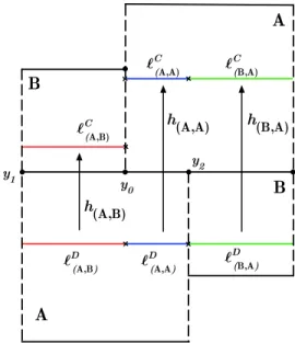
For every Markov rectangleM ∈ MG, choose an unstable spanning leaf segment
ℓ(x, M) inM for somex∈M. LetI={ℓM :M ∈ M}. For every pair (M, N)∈P, there are maximal leaf segmentsℓD
(M,N)⊂ℓM, ℓC(M,N)⊂ℓN such that the unstable holonomy h(M,N) : ℓD(M,N) → ℓC(M,N) is well defined. We call such holonomies h(M,N) : ℓD(M,N) → ℓC(M,N) the unstable primitive holonomies associated to the
Markov partition MG. The complete set of unstable holonomies HG consists of all stable primitive holonomies and their inverses. In Figure 10, we exhibit the complete set of unstable holonomies
HG =
h(A,A), h−(A1
,A), h(A,B), h−(A1
,B), h(B,A), h−(B1 ,A)
associated to the Markov partitionMG.
Figure 10. A complete set of unstable holonomiesHGassociated to the Markov partitionMG.
A diffeomorphismθ:I→Jis said to beC1+zygmundifθisC1and the derivative θ′ satisfies the zygmund condition, i.e. for all pointsx, y
∈I,
θ′(x) +θ′(y)
−2θ′
x+y
2
=χθ(|y−x|),
where the functionχθ is such that χθ(t)→0 when t→0. In particular, a C2+β diffeomorphism, withβ >0, is aC1+zygmund diffeomorphism. The importance of this smooth class follows from the fact that it corresponds to maps that distort cross-ratios of quadruples of points in I by an amount that iso(|I|) (see [7], [18] and [28]).
4.1. Proof of Theorem 1.3. By Lemma 3.3 and Theorem 4.1 in [22], ifGhas a
C1+zygmund complete system of unstable holonomies, thenσ
G =σGA. By Lemma 3.2, fori∈Nwith Fibonacci decompositionFn
0, . . . , Fnp, we have that the following conditions hold:
(i) If either (np = 1 and np−1 is odd) or (np = 2 and np−1 is even), then Ki∈BandKi+1∈A. Hence,ai =σGA(Ki:Ki+1) =γ
−1.
(ii) If either (np= 1 andnp−1 is even) or (np>2 andnp is odd), thenKi∈A andKi+1∈B. Hence, ai=σGA(Ki:Ki+1) =γ.
(iii) If either (np = 2 and np−1 is odd) or (np > 2 and np is even), then
Ki, Ki+1∈A. Hence, ai=σGA(Ki:Ki+1) = 1. Thus, from conditions (i), (ii) and (iii) we conclude that (aG
i )i∈Nis the rigid golden
sequence.
Acknowledgments
We are grateful to Alby Fisher, David Rand, Dennis Sullivan, Fl´avio Ferreira and Yunping Jiang for a number of very fruitful and useful discussions on this work and for their friendship and encouragement. We thank the LIAAD-INESC Porto LA, Calouste Gulbenkian Foundation, PRODYN-ESF, POCTI and POSI by FCT and the Minist´erio da Ciˆencia e da Tecnologia and the Pluriannual Funding Program of LIAAD-INESC Porto LA and of Research Centre of Mathematics of the University of Minho for their financial support. Part of this research was started during a visit by the authors to the IHES and CUNY, and continued at the Isaac Newton Institute, the University of Warwick, IMPA, MSRI and SUNY. We thank them for their hospitality.
References
[1] Anosov, D.V., Tangent fields of transversal foliations in U-systems, Math. Notes Acad. Sci., USSR,2(5) (1967). MR0242190 (39:3523)
[2] Bedford T., Fisher, A.M., Ratio geometry, rigidity and the scenery process for hyperbolic Cantor sets, Ergod. Th. & Dynam. Sys.,17, 531–564 (1997). MR1452179 (99b:58137) [3] Cawley, E., The Teichm¨uller space of an Anosov diffeomorphism ofT2, Inventiones
Mathe-maticae,112, 351–376 (1993). MR1213107 (94c:58141)
[4] Coullet, P. and Tresser, C., It´eration d’endomorphismes et groupe de renormalisation, J. de Physique,C5, 25 (1978).
[5] Feigenbaum, M., The universal metric properties of nonlinear transformations,J. Stat. Phys.,
21(1979), 669-706. MR555919 (82e:58072)
[6] Feigenbaum, M., Quantitative universality for a class of nonlinear transformations,J. Stat. Phys.,19(1978), 25-52. MR0501179 (58:18601)
[7] Jacobson, M.V., Swiatek, G., Quasisymmetric conjugacies between unimodal maps. I. In-duced expansion and invariant measures. Stony Brook preprint (1991).
[8] Jiang, Y., Asymptotic differentiable structure on Cantor set. Comm. in Math. Phys., 155
(3), 503–509 (1993). MR1231640 (94e:58100)
[9] Jiang, Y., Renormalization and Geometry in One-Dimensional and Complex Dynamics. Ad-vanced Series in Nonlinear Dynamics, Vol.10, World Scientific Publishing Co. Pte. Ltd., River Edge, NJ (1996). MR1442953 (98e:58070)
[10] Jiang, Y., Smooth classification of geometrically finite one-dimensional maps. Trans. Amer. Math. Soc.,348(6), 2391–2412 (1996). MR1321579 (96j:58054)
[11] Jiang, Y., On rigidity of one-dimensional maps. Contemporary Mathematics, AMS Series,
211, 319–431 (1997). MR1476995 (98h:58056)
[13] Jiang, Y., Teichm¨uller Structures and Dual Geometric Gibbs Type Measure Theory for Con-tinuous Potentials, preprint (2008).
[14] Jiang, Y., Cui, G., Gardiner, F., Scaling functions for degree two circle endomorphisms. Contemporary Mathematics, AMS Series,355, 147–163 (2004). MR2145061 (2006d:37067) [15] Jiang, Y., Cui, G., Quas, A., Scaling functions, Gibbs measures, and Teichm¨uller space of
circle endomorphisms, Discrete and Continuous Dynamical Systems,5, no. 3, 535–552 (1999).
MR1696328 (2000f:37023)
[16] Lanford, O., Renormalization group methods for critical circle mappings with general rotation number, VIIIth International Congress on Mathematical Physics (Maresille, 1986), World Sci. Publishing, Singapore (1987), 532-536. MR915597
[17] Ma˜n´e, R., Ergodic Theory and Differentiable Dynamics, Springer-Verlag, Berlin (1987). MR889254 (88c:58040)
[18] de Melo, W., van Strien, S., One-dimensional Dynamics. A series of Modern Surveys in Mathemaics, Springer-Verlag, New York (1993). MR1239171 (95a:58035)
[19] Pinto, A. A. and Rand, D. A., Renormalization gives all surface Anosov diffeomorphisms with a smooth invariant measure,submitted.
[20] Pinto, A. A. and Rand, D. A., Solenoid functions for hyperbolic sets on surfaces, Dynamics, Ergodic Theory and Geometry: Dedicated to Anatole Katok (ed. Boris Hasselblat) MSRI Publications,54(2007), 145-178. MR2369446 (2010b:37083)
[21] Pinto, A. A. and Rand, D. A., Geometric measures for hyperbolic sets on surfaces. Stony Brook preprint, (2006).
[22] Pinto, A. A. and Rand, D. A., Rigidity of hyperbolic sets on surfaces, J. London Math. Soc.,
71, 2 (2004), 481-502. MR2122440 (2005k:37051)
[23] Pinto, A. A. and Rand, D. A., Smoothness of holonomies for codimension 1 hyperbolic dynamics, Bull. London Math. Soc.,34(2002), 341-352. MR1887706 (2003a:37037)
[24] Pinto, A. A. and Rand, D. A., Teichm¨uller spaces and HR structures for hyperbolic surface dynamics, Ergod. Th. Dynam. Sys.22(2002), 1905-1931. MR1944410 (2004i:37055)
[25] Pinto, A. A. and Rand, D. A., ClassifyingC1+structures on dynamic fractals: 1 The moduli
space for solenoid functions for Markov maps on train-tracks, Ergod. Th. Dynam. Sys.15
(1995), 697-734. MR1346397 (97b:58094)
[26] Pinto, A. A., Rand, D. A., Ferreira, F., Fine structures of hyperbolic diffeomorphisms, Springer-Verlag Monograph (2008). MR2464147
[27] Pinto, A. A., Rand, D. A., Ferreira, F., Cantor exchange systems and renormalization, J. Differential Equations,243(2007), no. 2, 593–616. MR2371802 (2010d:37054)
[28] Pinto, A. A. and Sullivan, D., The circle and the solenoid. Dedicated to Anatole Katok on the Occasion of his 60th Birthday,DCDS-A16, 2 (2006), 463-504. MR2226493 (2009b:37074) [29] Rand, D. A., Global phase space universality, smooth conjugacies and renormalisation: 1.
TheC1+α
case,Nonlinearity,1(1988), 181-202. MR928952 (89g:58109)
[30] Schub, M., Global Stability of Dynamical Systems, Springer-Verlag (1987) MR869255 (87m:58086)
[31] Sullivan, D., Differentiable structures on fractal-like sets determined by intrinsic scaling func-tions on dual Cantor sets, Proceedings of Symposia in Pure Mathematics, 48, American
Mathematical Society (1988). MR974329 (90k:58141)
[32] Veech, W., Gauss measures for transformations on the space of interval exchange maps, The Annals of Mathematics, 2nd Ser.,115, 2 (1982), 201-242. MR644019 (83g:28036b)
[33] Williams, R. F., Expanding attractors. Publ. I.H.E.S., 43 (1974), 169-203. MR0348794
(50:1289)
Departamento de Matem´atica e LIAAD-INESC Porto LA, Faculdade de Ciˆencias, Uni-versidade do Porto, Rua do Campo Alegre, 687, 4169-007 Porto, Portugal
E-mail address:[email protected]
Escola Superior de Tecnologia e de Gest˜ao, Instituto Polit´ecnico de Braganc¸a, Campus de Santa Apol´onia, Ap. 1134, 5301-854 Braganc¸a, Portugal
E-mail address:[email protected]
Instituto de Matem´atica, Facultad de Ingenieria, CC30, CP 11300, Universidad de la Republica, Montevideo, Uruguay