Anosov and Circle Diffeomorphisms

Anosov and Circle Diffeomorphisms

Jo˜ao P. Almeida, Albert M. Fisher, Alberto A. Pinto and David A. Rand

Abstract We present an infinite dimensional space of C1+ smooth conjugacy classes of circle diffeomorphisms that areC1+_{fixed points of renormalization. We}

exhibit a one-to-one correspondence between theseC1+_{fixed points of}

renormaliz-ation andC1+_{conjugacy classes of Anosov diffeomorphisms.}

2.1 Introduction

The link between Anosov diffeomorphisms and diffeomorphisms of the circle is due to D. Sullivan and E. Ghys through the observation that the holonomies of Anosov diffeomorphisms give rise toC1+circle diffeomorphisms that areC1+fixed points of renormalization (see also [1]). A. Pinto and D. Rand [21] proved that this observation gives an one-to-one correspondence between the corresponding smooth

Jo˜ao P. Almeida

LIAAD-INESC Porto LA; Departamento de Matem´atica, Escola Suoerior de Tecnologia e de Gest˜ao, Instituto Polit´ecnico de Baganc¸a. Campus de Santa Apol´onia, Ap. 1134, 5301-857 Braganc¸a, Portugal.

e-mail: jpa@ipb.pt

Albert M. Fisher

Departamento de Matem´atica, IME-USP, Caixa Postal 66281, CEP 05315-970 S˜ao Paulo, Brasil. e-mail: afisher@ime.usp.br

Alberto A. Pinto

LIAAD-INESC Porto LA; Departamento de Matem´atica, Faculdade de Ciˆencias da Universidade do Porto, Rua do Campo Alegre, 687, 4169-007, Portugal; Departamento de Matem´atica e Centro de Matem´atica da Universidade do Minho, Campus de Gualtar, 4710-057 Braga, Portugal. e-mail: aapinto1@gmail.com

D. A. Rand

Warwick Systems Biology & Mathematics Institute, University of Warwick, Coventry CV4 7AL, United Kingdom.

e-mail: dar@maths.warwick.ac.uk

conjugacy classes. A key object in this link is the smooth horocycle equipped with a hyperbolic Markov map.

2.2 Circle Difeomorphisms

Fix a natural numbera_∈◆and let❙be acounterclockwise oriented circle homeo-morphic to the circle ❙1=❘/(1+γ)❩, where γ = (−a+√a2_+4)/2=1/(a+ 1/(a+···)). We note that if a=1 then γ is the inverse of the golden number (1+√5)/2. A key feature ofγis that it satisfies the relationaγ+γ2_=1.

Anarc in❙is the image of a non trivial intervalI in❘by a homeomorphism α:I_→❙. IfIis closed (resp. open) we say thatα(I)is aclosed(resp.open)arcin ❙. We denote by(a,b)(resp.[a,b]) the positively oriented open (resp. closed) arc in ❙starting at the pointa_∈❙and ending at the pointb_∈❙. AC1+atlasA _of❙_is

a set of charts such that (i) every small arc of❙is contained in the domain of some chart inA_{, and (ii) the overlap maps areC}1+α _{compatible, for someα>0.}

AC1+ _{circle diffeomorphismis a triple (g,❙,A)whereg:❙→❙ is aC}1+α

diffeomorphism, with respect to theC1+α _{atlasA, for someα>0, andgis}

quasi-symmetric conjugate to the rigid rotationrγ:❙1→❙1, with rotation number equal

toγ/(1+γ). We denote byF _{the set of all}C1+circle diffeomorphisms(g,❙,A_),

with respect to aC1+atlasA _in❙.

In order to simplify the notation, we will denote theC1+circle diffeomorphism (g,❙,A_{)only byg.}

2.2.1 The Horocycle and Renormalization

x

0

g2₍₀₎ g(0)

S

g3₍₀₎

p_g

H

S0

S2

S1

~

= S3

SH

2 SH

1 SH

0USH3

p_g(0)

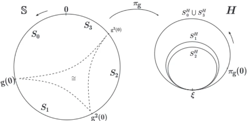
Fig. 2.1 The horocycleH for the casea=2. The junctionξ of the horocycle is equal toξ =

Let us mark a point in ❙ that we will denote by 0∈❙, from now on. Let

S0 = [0,g(0)] be the oriented closed arc in ❙, with endpoints 0 and g(0). For k=0, . . . ,alet Sk=

gk_(0),gk+1₍₀₎

be the oriented closed arc in❙, with endpoints gk(0)andgk+1(0)and such that Sk∩Sk₋1={gk(0)}. Let Sa+1=ga+1(0),0 be the oriented closed arc in❙, with endpointsga+1(0)and 0. We introduce an equi-valence relation_∼in❙by identifying thea+1 pointsg(0), . . . ,ga+1(0)and form the oriented topological spaceH(❙,g) =❙/∼. We call this oriented topological space thehorocycle(see Figure 2.1) and we denote it byH=H(❙,g). We consider the quotient topology inH. Let πg:❙→H be the natural projection. The point

ξ =πg(g(0)) =···=πg(ga+1(0))∈H is called thejunctionof the horocycleH.

Fork=0, . . . ,a+1, letSH

k =SHk(❙,g)⊂Hbe the projection byπgof the closed arc

Sk. AparametrizationinHis the image of a non trivial intervalIin❘by a

homeo-morphismα:I_→H. IfIis closed (resp. open) we say thatα(I)is aclosed(resp. open)arcinH. AchartinHis the inverse of a parametrization. Atopological atlas

B_{on the horocycleHis a set of charts{(j,J)}, on the horocycle, with the property}

that every small arc is contained in the domain of a chart inB_{, i.e. for any open}

arcKinHand anyx_∈Kthere exists a chart{(j,J)} ∈B_{such thatJ∩Kis a non}

trivial open arc inHandx_∈J_∩K. AC1+atlasB_{in H is a topological atlas}B

such that the overlap maps areC1+αand haveC1+α uniformly bounded norms, for someα>0.

x 0

g2(0) g(0)

S

g3(0) p_g

H

S0

S2

S1

~

=

S3

SH

2 SH

1

j : J a R i : I a R

0 R

J 1 L

p_g(J 1 L ₎

c

p_g(J₃R )

p_g(d)

J₃R

SH

0USH3

d

p_g(0) p_g(c)

LetA _{be aC}1+_{atlas in❙for whichgisC}1+_{. We are going to construct aC}1+

atlasAH _{in the horocycle that is theextended pushforwardA}H_{= (π}

g)_∗A of the

atlasA _in❙.

Ifx_∈H_\{ξ}then there exists a sufficiently small open arcJinH, containingx, such thatπ−1

g (J)is contained in the domain of some chart(I,i)inA. In this case,

we define (J,i_◦π−1

g )as a chart in AH. Ifx=ξ andJis a small arc containing

ξ, then either (i) π−1

g (J) is an arc in❙ or (ii) πg−1(J)is a disconnected set that

consists of a union of two connected components. In case (i),π−1

g (J)is connected

and we define J,i_◦π−1

g

as a chart inAH_{. In case (ii),π}−1

g (J)is a disconnected

set that is the union of two connected arcsJ_kLandJ_lRof the formJ_lR= [gl_(0),d)and

J_kL= (c,gk_{(0)], respectively, for somek,l∈ {0, . . . ,a+1}withk6=l(see Figure 2.2).}

Let(I,i)∈A _{be a chart such thatI⊃(c,d). We define j:J→}❘_{as follows,}

j(x) =

i_◦π−1

g (x), ifx∈πg([gl(0),d))

i_◦gl−k_◦π−1

g (x),ifx∈πg((c,gk(0)]) .

We call the atlas determined by these charts, theextended pushforward atlas ofA

and, by abuse of notation, we will denote it byAH_{= (π} g)_∗A.

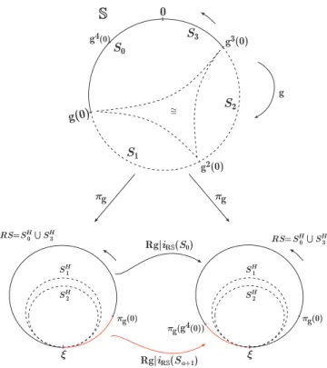
Letg= (g,❙,A_{)be aC}1+_{circle diffeomorphism with respect to aC}1+_atlasA

in❙. LetR❙=SH_0∪SH_a+1be projection byπgof the oriented close arcS0∪Sa+1of❙. LetiR❙:S0∪Sa+1⊂❙→R❙be the natural inclusion and letRA be the restriction,

A_|R❙, of theC1+_{atlasA toR❙. Therenormalization of g= (g,❙,A)is the triple}

(Rg,R❙,RA_{), where}Rg:R❙_→R❙is the map given by (see Figure 2.3),

iR❙◦ga+1=Rg◦iR❙, f or Rg|iR❙(S0), iR❙◦g=Rg◦iR❙, f or Rg|iR❙(Sa+1)

For simplicity of notation, we will denote the renormalization of aC1+circle diffeomorphismg,(Rg,R❙,RA_{), only byRg.}

We recall thatF _{denotes the set of allC}1+_{circle diffeomorphisms(g,❙,A)with}

respect to aC1+atlasA _in❙.

Lemma 2.1.The renormalization Rg of a C1+circle diffeomorphism g_∈F _{is a C}1+

circle diffeomorphism, i.e. the map R:F_→F _{given by R(g) =}Rg is well defined. In particular, the renormalization Rrγof the rigid rotation is the rigid rotation rγ.

The proof of Lemma 2.1 is in [21].

The marked point 0∈❙determines a marked point 0 in the circleR❙. SinceRg is homeomorphic to a rigid rotation, there existsh:❙→R❙, withh(0) =0, such thathconjugatesgandRg.

Definition 2.1.Ifh:❙_→R❙isC1+, we callgaC1+fixed point of renormalization. We will denote byR_{the set of all}C1+_{circle diffeomorphismsg∈F that areC}1+

fixed points of renormalization.

We note that the rigid rotationrγ, with respect to the atlasAiso, is an affine fixed

0

g2₍₀₎ g(0)

S

g3(0)

p_g S0

S2

S1

~

= S3

x

SH

2 SH

1

p_g(0)

SH

0USH3 RS=

x

SH

2 SH

1

p_g(0)

SH

0USH3 RS= p_g

g

p_g(g4(0)) g4(0)

Rg|iRS(S0)

Rg|iRS(Sa+1)

Fig. 2.3 The renormalizationRg= (Rg,R_❙,RA)of aC1+_{circle diffeomophismg= (g,❙,A).}

2.2.2 Markov Maps

Letg= (g,❙,A_{)be aC}1+_{circle diffeomorphism, with respect to aC}1+_atlasA,

andRg= (Rg,R❙,RA_{)its renormalization. LetH=}H(❙,_g)andRH=H(R❙,_Rg)

be the horocycles determined by theC1+_{circle diffeomorphismsgandRg,}

respect-ively. LetAH _andARH _{be the atlas in the horocyclesH andRH, that are the}

ex-tended pushforwards of the atlasesA _andRA_{, respectively. Let}iH:❙→Hbe the

natural inclusion.

Leth:❙→R❙be the homeomorphism that conjugates g andRgsending the marked point 0 ofgin the marked point 0 ofRg.

Definition 2.2.TheMarkov map Mgassociated to g∈F is the mapMg:H→H

defined by

Mg(x) =

iH◦h−1◦iRS◦iH−1(x),i f x∈iH(S0∪Sa+1)

iH◦h−1◦iRS◦g−k◦i_H−1(x),i f x∈iH(Sk),k=1, . . . ,a

.

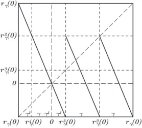
We observe that, in particular, the rigid Markov map Mrγ is an affine map with

respect to the atlasAH

rep-resented in Figure 2.4. We observe that the identification inH ofg(0)withg2(0) makes the Markov mapMga local homeomorphism.

0 0

r_g (0) r3

g (0)

g-g2 _g2 _{g g} r2

g (0) rg (0)

r_g (0)

r2

g (0)

r3

g (0)

r4

g (0)

g2

Fig. 2.4 The Markov mapMrγ with respect to the atlasA

H iso.

Lemma 2.2.Let g_∈F_{. The Markov map Mgassociated to g is a C}1+_local

diffeo-morphism with respect to the atlasAH_{= (π}

g)_∗A if, and only if, the diffeomorphism

g is a fixed point of renormalization.

The proof of Lemma 2.2 is in [21].

2.3 Anosov Diffeomorphisms

Fix a positive integer a_∈◆and consider theAnosov automorphism Ga: ❚→❚

given byGa(x,y) = (ax+y,x), where❚is equal to❘2/(v❩×w❩)withv= (γ,1)

andw= (−1,γ). Letπ: ❘2_{→❚be the natural projection. LetA}

0andB0be the rectangles[0,1]×[0,1]and[−γ,0]×[0,γ]respectively. A Markov partitionM_G

aof

Gais given byA=π(A0)andB=π(B0)(see Figure 2.5). The unstable manifolds of

Gaare the projection byπof the vertical lines in the plane, and the stable manifolds

ofGaare the projection byπof the horizontal lines in the plane.

AC1+Anosov diffeomorphism G:❚→❚is aC1+αdiffeomorphism, withα>0, such that (i)Gis topologically conjugate toGa; (ii) the tangent bundle has aC1+α

uniformly hyperbolic splitting into a stable direction and an unstable direction (see [39]). We denote by G _{the set of all suchC}1+ _{Anosov diffeomorphisms with an}

p(0,0)

A

g2

G₂(A)

g

w

v

B

g _B

g2

G₂(B)

A

Fig. 2.5 The Anosov automorphismG2:❚→❚.

If h is the topological conjugacy betweenGa andG, then a Markov partition

M_{G of} Gis given byh(A)andh(B). Letd =dρ be the distance on the torus❚,

determined by a Riemannian metric ρ. We define the mapGι =G if ι =u, or

Gι=G−1ifι=s. Forι∈ {s,u}andx∈❚, we denote the localι-manifolds through

xby

Wι(x,ε) =

y_∈❚:d(G−ιn(x),Gι−n(y))≤ε,for alln≥0 .

By the Stable Manifold Theorem (see [39]), these sets are respectively contained in the stable and unstable immersed manifolds

Wι(x) = [

n_≥0

Gn_ι Wι G−_ιn(x),ε0

which are the image ofC1+α immersionsκι,x:❘→❚, for some 0<α ≤1 and

some smallε0>0. Anopen(resp.closed)ι-leaf segment Iis defined as a subset of Wι(x)of the formκι,x(I1)whereI1is an open (resp. closed) subinterval (non-empty) in❘. Anι-leaf segmentis either an open or closedι-leaf segment. The endpoints of anι-leaf segmentI=κι,x(I1)are the pointsκι,x(u)andκι,x(v)whereuandv

2.3.1 Spanning Leaf Segments

One can find a small enoughε0>0, such that for every 0<ε<ε0there isδ = δ(ε)>0 with the property that, for all pointsw,z_∈❚withd(w,z)<δ,Wu_(w,ε)

andWs_{(z,ε)intersect in a unique point that we denote by}

[w,z] =Wu(w,ε)∩Ws(z,ε).

Arectangle Ris a subset of❚which is (i) closed under the bracket, i.e.x,y∈R_⇒ [x,y]∈R, and (ii) proper, i.e. it is the closure of its interior in❚. Ifℓu_andℓs _are

respectively unstable and stable closed leaf segments intersecting in a single point then we denote by[ℓu_{, ℓ}s_{]the set consisting of all points of the form[w,z]withw∈ℓ}u

andz_∈ℓs_{. We note that[ℓ}u_{, ℓ}s_{]is a rectangle. Conversely, given a rectangleR, for}

eachx_∈Rthere are closed unstable and stable leaf segments of❚,ℓu_(x,R)⊂Wu_(x)

andℓs_(x,R)⊂Ws_{(x)such thatR= [ℓ}u_{(x,R), ℓ}s_{(x,R)]. The leaf segmentsℓ}u_(x,R)

andℓs_{(x,R)are called, respectively,unstableandstable spanning leaf segments.}

R

x z

l

l

q(w)=[w,z] w

l

l

Fig. 2.6 A basic stable holonomyθ:ℓu_(x,R)→ℓu_(z,R).

2.3.2 Basic Holonomies

Suppose thatxandzare two points inside any rectangleRof ❚. Letℓs_(x,R)and

ℓs_{(z,R)be two stable spanning leaf segments ofRcontaining, respectively,xand}

z. We define the mapθ:ℓs_(x,R)→ℓs_{(z,R)byθ(w) = [w,z](see Figure 2.6). Such}

2.3.3 Lamination Atlas

Thestable lamination atlasLs_=Ls_{(G,ρ), determined by a Riemannian metric}

ρ, is the set of all mapse:I_→❘, where eis an isometry between the induced Riemannian metric on the stable leaf segmentI and the Euclidean metric on the reals. We call the mapse_∈Ls_{thestable lamination charts. Similarly, we can define}

theunstable lamination atlasLu₌Lu_{(G,ρ). By Theorem 2.1 in [27], the basic}

unstable and stable holonomies areC1+with respect to the lamination atlasLs_.

2.3.4 Circle Diffeomorphisms

LetG_∈G _{be aC}1+_{Anosov diffeomorphism with an invariant measure absolutely}

continuous with respect to the Lebesgue measure and topologically conjugate to the Anosov automorphismGa by the homeomorphismh. For each Markov rectangle

R, lett_Rs be the set of all unstable spanning leaf segments ofR. Thus, by the local product structure, one can identifyts

Rwith any stable spanning leaf segmentℓs(x,R)

ofR. We form the space❙Gby taking the disjoint uniont_hs_(A)Ft_hs_(B), whereh(A)

andh(B)are the Markov rectangles of the Markov partitionM_{G, and identifying}

two pointsI_∈t_Rs andJ_∈t_Rs_′ if (i)R₆=R′, (ii) the unstable leaf segmentsIandJare unstable boundaries of Markov rectangles, and (iii) int(I∩J)6=/0. Topologically, the space❙Gis acounterclockwise oriented circle. Letπ❙G:

F

R∈M_GR→❙Gbe the

natural projection sendingx_∈Rto the pointℓu_(x,R)in❙ G.

LetI_❙ be an arc of❙G andI a leaf segment such thatπ❙G(I) =I❙. The chart

i:I_→❘inL ₌Ls_{(G,ρ)determines acircle chart i}

❙:I_❙→❘forI_❙ given by i_❙◦π❙G =i. We denote byAG=A(G,ρ)the set of all circle chartsi❙determined

by chartsiinL ₌Ls_{(G,ρ). Given any circle chartsi}

❙:I_❙→❘and j_❙:J_❙→❘, the overlap map j_❙◦i−_❙1:i_❙(I❙∩J_❙)→ j_❙(I❙∩J_❙)is equal to j_❙◦i_❙−1=j_◦θ_◦i−1, wherei=i_❙◦π_❙G:I_→❘and j= j_❙◦π_❙G:J_→❘are charts inL_{, and}

θ:i−1(i_❙(I_❙∩J_❙))→ j−1(j_❙(I_❙∩J_❙))

is a basic stable holonomy. By Theorem 2.1 in [27], there existsα>0 such that, for all circle chartsi_❙ and j_❙ inA_{G, the overlap maps j❙◦i}−1

❙ = j◦θ◦i−1areC1+α diffeomorphisms with a uniform bound in theC1+α norm. Hence,A_G=A_(G,ρ)

is aC1+atlas.

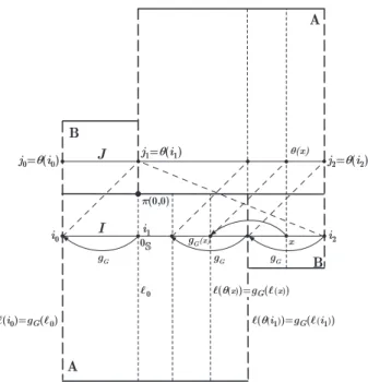
Suppose thatIandJare stable leaf segments andθ:I_→Jis a holonomy map such that, for everyx_∈I, the unstable leaf segments with endpointsxandθ(x)cross once, and only once, a stable boundary of a Markov rectangle. We define thearc ro-tation mapθ˜G:π❙G(I)→π❙G(J), associated toθ, by ˜θG(π❙G(x)) =π❙G(θ(x))(see

Figure 2.7). By Theorem 2.1 in [27] there exists α >0 such that the holonomy θ :I_→J is a C1+α _{diffeomorphism, with respect to the C}1+ _{lamination atlas}

Ls_{(G,ρ). Hence, the arc rotation maps ˜θ}

GareC1+diffeomorphisms, with respect

p(0,0)

A

B B

A

0S

i0

gG

gG(x) j0=q(i0)

i2

j2=q(i2)

x

q(x)

J

I

l₀

i1

j1=q(i1)

gG gG

l(i0)=gG(l0)

l(q(x))=gG(l(x))

l(q(i1))=gG(l(i1))

Fig. 2.7 The arc rotation mapgG=θ˜G:π❙G(I)→π❙G(J). We note that❙=π❙G(I) =π❙G(J)and

ℓ(x) =π_❙G(x)is the unstable spanning leaf segment containingx.

Lemma 2.3.There is a well-defined C1+circle diffeomorphism gG, with respect to

the C1+atlasA_G=A_{(G,ρ), such that gG|π❙}

G(I) =θ˜G, for every arc rotation map

˜

θG. In particular, if Gais the Anosov automorphism, then gGa is the rigid rotation

rγ, with respect to the isometric atlasAiso=A(Ga,E), where E corresponds to the

Euclidean metric in the plane.

The proof of Lemma 2.3 is in [21].

2.3.5 Train-Tracks and Markov Maps

Roughly speaking, train-tracks are the optimal leaf-quotient spaces on which the stable and unstable Markov maps induced by the action ofGon leaf segments are local homeomorphisms.

LetG_∈G _{be a}C1+Anosov diffeomorphism. Lethbe the homeomorphism that conjugatesGwithGa. We recall that, for each Markov rectangleR,tRs denotes the

set of all unstable spanning leaf segments ofRand, by the local product structure, one can identifyt_Rs with any stable spanning leaf segmentℓs_{(x,R)ofR. We form}

Markov rectangles of the Markov partitionM_{Gand identifying two pointsI∈t}s Rand

J_∈t_Rs′ if (i) the unstable leaf segmentsIandJare unstable boundaries of Markov

rectangles and (ii)int(I∩J) =/0. This space is called thestable train-trackand it is denoted byTG.

LetπTG :

F

R∈M_GR→TG be the natural projection sending the pointx∈Rto

the point ℓu_(x,R)inT

G. A topologically regular point I inTG is a point with a

unique preimage underπTG(i.e. the preimage ofIis not a union of distinct unstable

boundaries of Markov rectangles). If a point has more than one preimage byπTG,

then we call it ajunction. Hence, there is only one junction.

A charti:I_→❘inL ₌Ls_{(G,ρ)determines atrain-track chart i}

T:IT→❘for

IT given byiT◦πTG=i. We denote byA

TG₌ATG_{(G,ρ)the set of all train-track}

chartsiT determined by chartsiinL =Ls(G,ρ). Given any train-track chartsiT:

IT→❘andjT:JT→❘inATG, the overlap map jT◦iT−1:iT(IT∩JT)→jT(IT∩JT)

is equal to jT◦i−T1=j◦θ◦i−1, wherei=iT◦πTG:I→❘andj=jT◦πTG:J→❘

are charts inL_{, and}

θ:i−1(iT(IT∩JT))→ j−1(jT(IT∩JT))

is a basic stable holonomy. By Theorem 2.1 in [27] there existsα>0 such that, for all train-track chartsiT and jT inATG(G,ρ), the overlap maps jT◦i−T1= j◦θ◦

i−1haveC1+α diffeomorphic extensions with a uniform bound in theC1+α norm. Hence,ATG_{(G,ρ)is aC}1+α_{atlas inT}

G.

The(stable) Markov map MG:TG→TGis the mapping induced by the action

of Gon unstable spanning leaf segments, that it is defined as follows: ifI_∈TG,

MG(I) =πTG(G(I))is the unstable spanning leaf segment containing G(I). This

map MG is a local homeomorphism because Gsends short stable leaf segments

homeomorphically onto short stable leaf segments.

Astable leaf primary cylinder of a Markov rectangle Ris a stable spanning leaf segment ofR. Forn_≥1, astable leaf n-cylinder of Ris a stable leaf segmentIsuch that (i)GnI is a stable leaf primary cylinder of a Markov rectangleR′(I)∈M_G;

(ii)Gn(ℓu_(x,R))⊂R′_{(I)for everyx∈I, whereℓ}u_{(x,R)is an unstable spanning leaf}

segment ofR.

Forn_≥1, an n-cylinder is the projection intoTG of a stable leafn-cylinder

segment. Thus, each Markov rectangle in❚projects in a unique primary stable leaf segment inTG.

Given a topological chart(e,U)on the train-trackTGand a train-track segment

C_⊂U, we denote by|C_|ethe length ofe(C). We say thatMGhasbounded geometry

in aC1+atlasA_{, if there isκ1>0 such that, for everyn-cylinderC1andn-cylinder}

C2with a common endpoint withC1, we haveκ1−1<|C1|e/|C2|e<κ1, where the

lengths are measured in any chart(e,U)of the atlas such thatC1∪C2⊂U. We note thatMGhas bounded geometry, with respect to aC1+atlasA, if, and only if, there

are κ2>0 and 0<ν<1 such that|C_|e≤κ2νn, for everyn-cylinder and every

e_∈B_.

By Section 4.3 in Pinto-Rand [25], we obtain thatMGisC1+and hasbounded

geometryinATG(G,ρ_{). In [21] it is proved thatM}

Definition 2.2. Hence,gGis a fixed point of renormalization. Futhermore, in [21] it

is proved that the mapG_→gGinduces an one-to-one correspondence betweenC1+

conjugacy classes of Anosov diffeomorphisms with an invariant measure absolutely continuous with respect to the Lebesgue measure and C1+ _{conjugacy classes of}

circle diffeomorphisms that are fixed points of renormalization.

We recall that G _{denotes the set of} C1+ Anosov diffeomorphisms Gthat are topologically conjugate to the linear Anosov automorphismGaand have an invariant

measure absolutely continuous with respect to the Lebesgue measure.

Theorem 2.1.For every G_∈G, the C1+_{circle diffeomorphism g}

Gis a C1+fixed

point of renormalization, with respect to the C1+_atlasA

G=A(G,ρ).

The proof of Theorem 2.1 is in [21].

Acknowledgments

Previous versions of this work were presented in the International Congresses of Mathematicians ICM 2006 and 2010, EURO 2010, ICDEA 2009 and in the celebra-tion of David Rand’s 60th birthday, achievements and influence, University of War-wick. We are grateful to Dennis Sullivan and Fl´avio Ferreira for a number of very fruitful and useful discussions on this work and for their friendship and encour-agement. We thank LIAAD-INESC Porto LA, Calouste Gulbenkian Foundation, PRODYN-ESF, POCTI and POSI by FCT and Minist´erio da Ciˆencia e da Tecnolo-gia, and the FCT Pluriannual Funding Program of the LIAAD-INESC Porto LA and of the Research Centre of Mathematics of University of Minho, for their financial support. A. Fisher would like to thank FAPESP, the CNPQ and the CNRS for their financial support.

References

1. Cawley, E.: The Teichm¨uller space of an Anosov diffeomorphism ofT2. Inventiones Math-ematicae,112, 351–376 (1993).

2. Coullet, P. and Tresser, C.: It´eration d’endomorphismes et groupe de renormalisation.J. de Physique, C5 25 (1978).

3. de Faria, E., de Melo, W. and Pinto, A. A.: Global hyperbolicity of renormalization forCr

unimodal mappings.Annals of Mathematics, 164 731-824 (2006).

4. Feigenbaum, M.: Quantitative universality for a class of nonlinear transformations.J. Stat. Phys., 19 25-52 (1978).

5. Feigenbaum, M.: The universal metric properties of nonlinear transformations.J. Stat. Phys., 21 669-706 (1979).

8. Franks, J.: Anosov diffeomorphisms. In: Smale, S. (ed) Global Analysis.14AMS Providence, 61–93 (1970).

9. Ghys, E.: Rigidit´e diff´erentiable des groupes Fuchsiens. Publ. IHES78, 163–185 (1993). 10. Jiang, Y., Metric invariants in dynamical systems.Journal of Dynamics and Differentiable

Equations, 17 1 5171 (2005).

11. Lanford, O., Renormalization group methods for critical circle mappings with general rota-tion number. VIIIth Internarota-tional Congress on Mathematical Physics.World Sci. Publishing, Singapore, 532-536 (1987).

12. de la Llave, R.: Invariants for Smooth conjugacy of hyperbolic dynamical systems II. Com-mun. Math. Phys.,1093, 369–378 (1987).

13. Manning, A.: There are no new Anosov diffeomorphisms on tori. Amer. J. Math.,96, 422 (1974).

14. Marco, J.M., Moriyon, R.: Invariants for Smooth conjugacy of hyperbolic dynamical systems I. Commun. Math. Phys.,109, 681–689 (1987).

15. Marco, J.M., Moriyon, R.: Invariants for Smooth conjugacy of hyperbolic dynamical systems III. Commun. Math. Phys.,112, 317–333 (1987).

16. de Melo, W.: Review of the bookFine structure of hyperbolic diffeomorphisms, by A. A. Pinto, D. Rand, and F. Ferreira, Springer Monographs in Mathematics.Bulletin of the AMS, S 0273-0979 01284-2 (2010).

17. de Melo, W. and Pinto, A.: Rigidity ofC2infinitely renormalization for unimodal maps.

Communications of Mathematical Physics, 208 91-105 (1999).

18. Penner, R. C. and Harer, J. L.:Combinatorics of Train-Tracks. Princeton University Press, Princeton, New Jersey (1992).

19. Pinto, A. A.: Hyperbolic and minimal sets,Proceedings of the 12th International Conference on Difference Equations and Applications, Lisbon, World Scientific, 1-29 (2007).

20. Pinto, A. A., Almeida, J. P. and Portela, A.: Golden tilings, Transactions of the AMS (to appear).

21. Pinto, A. A. and Rand, D. A.: Renormalisation gives all surface Anosov diffeomorphisms with a smooth invariant measure (submitted).

22. Pinto, A. A. and Rand, D. A.: Train tracks withC1+_{Self-renormalisable structures.Journal}

of Difference Equations and Applications(to appear).

23. Pinto, A. A. and Rand, D. A.: Train-tracks withC1+self-renormalisable structures.Journal of Difference Equations and Applications, 1-18 (2009).

24. Pinto, A. A. and Rand, D. A.: Solenoid functions for hyperbolic sets on surfaces. Dynamics, Ergodic Theory and Geometry, Boris Hasselblat (ed.),MSRI Publications, 54 145-178 (2007). 25. Pinto, A. A. and Rand, D. A.: Geometric measures for hyperbolic sets on surfaces.Stony

Brook preprint, 1-59 (2006).

26. Pinto, A. A. and Rand, D. A.: Rigidity of hyperbolic sets on surfaces.J. London Math. Soc., 71 2 481-502 (2004).

27. Pinto, A. A. and Rand, D. A.: Smoothness of holonomies for codimension 1 hyperbolic dy-namics.Bull. London Math. Soc., 34 341-352 (2002).

28. Pinto, A. A. and Rand, D. A.: Teichm¨uller spaces and HR structures for hyperbolic surface dynamics.Ergod. Th. Dynam. Sys, 22 1905-1931 (2002).

29. Pinto, A. A. and Rand, D. A.: Existence, uniqueness and ratio decomposition for Gibbs states via duality. Ergod.Th.&Dynam. Sys.21 533-543 (2001).

30. Pinto, A. A. and Rand, D. A.: ClassifyingC1+_{structures on dynamical fractals, 1. The moduli}

space of solenoid functions for Markov maps on train tracks. Ergod.Th.&Dynam. Sys., 15 697-734 (1995).

31. Pinto, A. A. and Rand, D. A.: ClassifyingC1+_{structures on dynamical fractals, 2. Embedded}

trees. Ergod.Th.&Dynam. Sys.15 969-992 (1995).

32. Pinto, A. A., Rand, D. A. and Ferreira, F.:C1+_{self-renormalizable structures.}

Communic-ations of the Laufen Colloquium on Science 2007. A. Ruffing, A. Suhrer, (eds.):J. Suhrer, 1-17 (2007).

34. Pinto, A. A. Rand, D. A., Ferreira, F.:Fine structures of hyperbolic diffeomorphisms. Springer Monograph in Mathematics, Springer (2009).

35. Pinto, A. A., Rand, D. A. and Ferreira, F.: Hausdorff dimension bounds for smoothness of holonomies for codimension 1 hyperbolic dynamics.J. Differential Equations, 243 168-178 (2007).

36. Pinto, A. A., Rand, D. A. and Ferreira, F., Cantor exchange systems and renormalization.J. Differential Equations, 243 593-616 (2007).

37. Pinto, A. A. and Sullivan, D.: The circle and the solenoid. Dedicated to Anatole Katok On the Occasion of his 60th Birthday.DCDS A, 16 2 463-504 (2006).

38. Rand, D. A.: Global phase space universality, smooth conjugacies and renormalisation, 1. The

C1+αcase. Nonlinearity, 1 181-202 (1988).

39. Schub, M.:Global Stability of Dynamical Systems. Springer-Verlag, (1987).

40. Thurston, W.: On the geometry and dynamics of diffeomorphisms of surfaces.Bull. Amer. Math. Soc., 19 417-431 (1988).

41. Veech, W.: Gauss measures for transformations on the space of interval exchange maps.The Annals of Mathematics, 2nd Ser.115 2 201-242 (1982).