Location of Vertically-Linked Oligopolists
André Barreira da Silva Rocha
1José Pedro Pontes
2Abstract
This paper examines the equilibrium of location of N vertically-linked firms. In a spatial economy composed of two regions, a monopolist firm supplies an input to N consumer goods firms that compete in quantities. It was concluded that, when there are increases in the transport cost of the input, downstream firms prefer to agglomerate in the region where the upstream firm is located, in order to obtain savings in the production cost. On the other hand, increases in the general transport cost or in the number of downstream firms lead to a dispersion of these firms, in order to reduce competition and locate closer to the final consumer.
Keywords: Agglomeration, Intermediate Goods, Spatial Oligopoly. J. E. L. Classification: R30, L13, C72.
Authors’ affiliation: 1Instituto Superior de Economia e Gestão, Technical University of Lisbon; 2Instituto Superior de Economia e Gestão, Technical University of Lisbon and Researcher, Research Unit on Complexity in Economics (UECE), corresponding author. Mailing Address: Instituto Superior de Economia e Gestão, Rua Miguel Lupi, 20, 1249-078 Lisboa, Portugal.
Tel. +351 21 3925916 Fax. +351 21 3922808
1 – Introduction
In the absence of labour mobility, the agglomeration of productive activity results from interactions between firms. As noted by MARSHALL (1920), these interactions can take the form of an exchange of intermediate goods. In this case, the saving in the transport cost of intermediate goods is a powerful incentive for the agglomeration of vertically-linked firms. In the literature that addresses this issue, the locational interaction of vertically-linked firms is modelled in the following way. There are two regions where the firms can locate, and an imperfectly competitive upstream industry supplies an intermediate good to the downstream industry, whose firms produce a final consumer good and can be either perfectly or imperfectly competitive. As far as the upstream industry is concerned, its market structure can be a Cournot oligopoly, as in AMITI (2001) and BELLEFLAMME and TOULEMONDE (2003), exhibit the characteristics of Dixit-Stiglitz monopolistic competition, as in FUJITA and HAMAGUCHI (2001), FUJITA and THISSE (2002) and VENABLES (1996), or it can contain only a single monopolist firm, as in PONTES (2003) and PONTES (2005). As far as the downstream industry is concerned, AMITI (2001), FUJITA and HAMAGUCHI (2001) and FUJITA and THISSE (2002) assume that this is perfectly competitive, while VENABLES (1996) and BELLEFLAMME and TOULEMONDE (2003) make the opposite assumption.
Under this framework, there are some effects that may lead to the dispersion or agglomeration of firms. According to VENABLES (1996), in vertically-linked industries, the downstream constitutes the market for the upstream, thus creating an incentive for the location of upstream firms in a region where there is a significant number of downstream firms. This effect is called the demand linkage between firms. At the same time, the downstream firms incur lower production costs if they locate close to the upstream firms, since they save the transport cost of the input. This is referred to as the cost linkage between firms. Combining the cost and demand linkages, a centripetal force appears, inducing the creation of an industrial cluster in one of the regions. According to PONTES (2005), the strength of the cost linkage is proportional to the transport cost of the input. On the other hand, the dispersion of final consumer demand, together with the competition effect, creates a centrifugal force leading to the dispersion of firms, in order to locate closer to local final consumers and simultaneously relax intra-regional competition. According to PONTES (2005), the incentive to disperse is greater when the transport cost of the final good is higher. The overall balance between these two forces is then responsible for the existence, the number of firms and the stability of the geographical equilibrium of location. Changes in the parameters that affect this spatial economy can lead to significant changes in this equilibrium.
According to PONTES (2005), a common assumption in this literature is that the transport costs of the input and of the final good vary independently, but a more real assumption is to consider that they vary in proportion to one another, since they are both influenced by the general quality of the transport and communication infrastructure.
In this paper, a monopolist firm supplies an intermediate good to N downstream firms that compete in quantities à la Cournot in the market for the final good. According to MAYER (2000), the literature about locational strategies involves models in which the competition is oligopolistic à la Bertrand and models in which it is oligopolistic à la Cournot. This latter kind of model is more realistic since it involves overlapping markets with the existence of intra-regional trade and the equilibrium of agglomeration of firms tends to occur in a central region, as in the real world. In the spatial economy assumed in this paper, firstly the firms select their locations simultaneously. Then, the upstream monopolist firm selects the delivered price of the input and, finally, the downstream firms take this price as given and compete among themselves, establishing the quantities to be supplied in each market. The transport costs of the input and the final good vary in proportion to one another.
This paper follows the analysis made in a paper by PONTES (2005), in which a similar model of vertically-linked industries was presented. In contrast with the former, this model develops a generalized model for the case in which all downstream firms are producing for both regions, allowing for the existence of N firms in the downstream industry instead of only the case of a duopoly. This generalization allows for a more realistic watch on the effects of downstream competition. Also, unlike the former paper, which only assessed whether or not there existed full agglomeration equilibrium of firms for different values of transport costs, this paper attempts to characterize the full set of equilibria of the location game.
Basically, when faced with increases in the transport cost of the input, downstream firms prefer to agglomerate in the region where the upstream firm is located in order to obtain savings in the production cost. On the other hand, increases in the transport cost of the final good lead to a dispersion of downstream firms, in order to reduce competition and locate close to the final consumer. Furthermore, it is not possible for there to exist a large industrial cluster in the region where the upstream firm is not located, showing the difficulty that countries with a less developed upstream industry have in being an attractive location for an industrial cluster. The structure of the paper is divided in the following manner: in section 2, the hypothesis of the model and a three-stage noncooperative game is presented; in section 3, we present the results of the model applied to the case of a spatial economy with fifty downstream firms; in section 4, we draw our conclusions.
2 – The model
2.1 – Hypothesis
1 – There are two symmetrical regions labelled A and B, each with the same number of final consumers;
this monopolist firm selects the delivered price wk (k = a, b), which maximizes its profit. There are N firms in the downstream industry, where N is an even number, and they compete in quantities à la Cournot. Each firm has to select in which of the two regions to locate its production plant. Once this selection has been made, the downstream industry is partitioned into two subsets, each of them with its typical firm i ∈ A; j ∈ B, and each region contains a number of downstream firms Nk,(k=a,b;Na ∪Nb =N;Na ∩Nb =∅). Independently of their location, the downstream firms supply each region. The quantity sold by a final producer
i (i = 1, 2, …, N) in region k (k = a, b) is given by qik. The total quantity of the final good sold in region k is given by
∑
∑
∈ ∈
+ =
a b
N
i j N
jk ik
k q q
Q , and we also define: i k ik
k Q q
Q− = − ;
jk k j
k Q q
Q− = − ;
3 – The firms in both industries do not have fixed costs, and the marginal cost of downstream firms is constant and equal to the price of the intermediate good (input) w, defined by the upstream firm, whose marginal cost is also constant and equal to c;
4 – In each region, each final consumer has a linear demand function and the price in each region is given bypk =1−Qk;Qk <1;
5 – Each firm transports and delivers its own product and the transport cost per unit of distance per unit of product is given by t for the final good and by γ for the intermediate good, where γ∈ (0, 1);
6 – The location decision is taken simultaneously by all the firms, so no firm has any information relating to the location of the other firms before it has taken its decision;
Without loss of generality, it is assumed that c = 0.
Based on these assumptions, this economy can be modelled through a three-stage game: in the first stage, the firms simultaneously select their locations; in the second stage, the upstream monopolist firm selects the delivered price of the input; and, in the third stage, the downstream firms take this price as given and compete among themselves, defining the quantities to be supplied in each market. The game is solved by backward induction.
2.2 – Solving the model
In the solution of the model, without any loss of generality, all the equations were defined while taking into account the fact that the upstream firm is located in region A. The full set of calculations is available to interested readers and may be obtained from the corresponding author upon request.
2.2.1 – 3rd stage of the game: defining the quantities to be supplied in each market The profit function of a typical downstream firm i∈A is given by:
(
)
(
a)
ibi b ib ia
a i a ia d
i = −q −Q −w q + −q −Q −w −t q
− −
1 1
The profit function of a typical downstream firm j∈B is given by:
(
)
(
b)
jbj b jb ja
b j a ja d
j = −q −Q −w −t q + −q −Q −w q
− −
1 1
π (2)
In equations (1) and (2), according to hypothesis 2:
jb b j b ib
b i b ja
a j a ia a i
a Q q Q Q q Q Q q Q Q q
Q− = − ; − = − ; − = − ; − = −
We also define:
(
)
(
)
∆ − =
∆ + = ⇒
∆ = −
+ =
2 2
N N N
N N N N
N N
N N N
b a
b a
b a
Maximizing the profit function defined in (1) in relation to qia and qib:
(
a)
ia b ja aia d
i N q N q w
q = ⇒ + + = −
∂ ∂
1 1
0 π
(3)
(
N)
q N q w tqib a ib b jb a
d
i = ⇒ + + = − −
∂ ∂
1 1
0 π
(4)
Maximizing the profit function defined in (2) in relation to qja and qjb:
(
N)
q w tq N
qja a ia b ja b
d
j = ⇒ + + = − −
∂ ∂
1 1 0
π
(5)
(
b)
jb bib a jb
d j
w q
N q N
q = ⇒ + + = −
∂ ∂
1 1 0
π
(6)
Two systems of equations are originated. The first one is obtained from (3) and (5), the solution of which gives:
(
)
(
)(
)
(
1)
2
2 2
*
+
+ +
∆ + − ∆ + + =
N
t w N N w N N
q a b
ja (7)
(
)
(
)(
)
(
1)
2 2 2
*
+
+ ∆
− + + ∆ − − =
N
t w N N w N N
q a b
ia (8)
The second system of equations is obtained from (4) and (6), the solution of which gives:
(
)(
) (
)
(
1)
2
2 2
*
+
+ ∆ + − + ∆
+ + =
N
w N N t w N N
q a b
(
)(
) (
)
(
1)
2 2 2
*
+
∆ − + + +
∆ − − =
N
w N N t w N N
q a b
ib (10)
Observing equations (7) to (10), it can be seen that:
(
qia*;q*ib;q*ja;q*jb)
= f(
N;∆N;wa( ) ( )
;wb ;t)
where N is a constant that depends on the number of downstream firms, whose value is previously defined at the beginning of the problem. So:
(
qia*;qib*;q*ja;q*jb)
= f(
∆N;wa( ) ( )
;wb ;t)
As wa;wb = f
( )
γ;t , a result that will be presented later, we have:(
qia*;qib*;q*ja;q*jb)
= f(
∆N;γ;t)
2.2.2 – 2nd stage of the game: selection of the prices wa and wb by the monopolist
upstream firm
Proposition 1: the upstream firm always selects the region with the larger number of downstream firms.
Proof: If a large number of downstream firms is located in region A, for example, a change of location by the upstream firm to region B is never profitable because, since the larger number of downstream firms is located in A, the input demand in region A is higher than the demand in region B. If the upstream firm moves from region A to region B, it has to address the same input demand as in region A, whilst bearing an additional transport cost, since, according to hypothesis 5, each firm is responsible for the transport of its own product.
Assuming the upstream firm is located in region A (without any loss of generality), its profit function is given by:
(
ia ib)
a(
b)
(
ja jb)
b au
N q q t w N q q
w + + − +
= γ
π1
Substituting the equations obtained in (7) to (10) of the previous section:
(
)
(
)(
)
(
)(
) (
)
(
)
(
)
(
)
(
)(
(
)
)
(
)(
) (
)
bb a
b a
b
a b a
b a
a u
N N
w N N t w N N t
w N N w N N t
w
N N
w N N t w N N t
w N N w N N w
+
+ ∆ + − + ∆
+ + + + +
∆ + − ∆ + + − +
+
+
∆ − + + +
∆ − − + + ∆
− + + ∆ − − =
1 2
2 2
2 2
1 2
2 2
2 2
1
(
)
{
[
(
)
(
)
]
(
)
(
b)(
)
[
b(
)
a(
)
b]
}
b a
a a
u
w N N w N N t w N
N t w
N N w N N w N N t w w
N
∆ + − ∆
+ + − − ∆ − −
+
+ ∆ + ∆
− + ∆ − − − − +
= ⇒
2 2
2 4 4
2 2
2 4 4 1 4
1 1
γ π
Maximizing the profit in the above equation in relation to price wa:
(
)
(
)
[
(
)
γ]
π
N N t w
N N w N N
wa a b
u
∆ − + − = ∆
− − + ∆ − ⇒
= ∂ ∂
1 2 4 4
2 4
0
1 (11)
Maximizing the profit function in relation to the price wb:
(
N N)
w(
N N)
w t t(
N N)
twb a b
u
γ γ
π = ⇒ − +∆ + +∆ + = − + + +∆
∂ ∂
2 4 2 4 2 4
4 0
1 (12)
From equations (11) and (12), we obtain a system of equations, the solution of which defines the expressions of wa e wb as being:
4 2 1
* t
wa = − (13)
(
t t)
wb 2 2γ
4 1
* = − + (14)
Based on equations (13) and (14), the prices of the intermediate good (input) are independent of the number of downstream firms located in each region. They only depend on the transport costs. So, wa;wb = f
( )
γ;t , which confirms that(
qia*;qib*;q*ja;q*jb)
= f(
∆N;γ;t)
, as was mentioned in the previous section.Moreover, equations (13) and (14) are in keeping with the expressions obtained for the input prices in PONTES (2005) in his model, developed for the case of only two downstream firms. The independence between the input prices and the number of downstream firms located in each region is also in accordance with the result obtained in BELLEFLAMME and TOULEMONDE (2003), where the equilibrium input prices were independent of the product variety selection made by the final producers.
Substituting equations (13) and (14) in equations (7) to (10), we obtain: From equation (7):
(
)
(
)
(
1)
2
2 4 2 1 2 4
2 1 2
*
+
− + +
+ ∆ + − − ∆ + + =
N
t t t N
N t N N qja
γ
(
) (
)(
)
[
]
(
1)
4
2 2
3 2 *
+
+ ∆ + + + − = ⇒
N
N N t
From equation (8):
(
)
(
)
(
1)
2 2 4 2 1 4 2 1 2 2 * + − + + ∆ − + − + ∆ − − = N t t t N N t N N qia γ
(
)(
)
[
]
(
1)
4 2 1 2 * + + ∆ − + + = ⇒ N N N t
qia γ (16)
From equation (9):
(
)
(
)
(
1)
2 2 4 2 1 2 4 2 1 2 * + − + + ∆ + − − + ∆ + + = N t t N N t t N N qjb γ
(
) (
)(
)
[
]
(
1)
4 2 2 1 2 * + − ∆ + + − + = ⇒ N N N t
qjb γ γ (17)
From equation (10):
(
)
(
)
(
1)
2 2 4 2 1 4 2 1 2 2 * + − + ∆ − + − + + ∆ − − = N t t N N t t N N qib γ
(
)(
)
[
]
(
1)
4 2 3 2 * + − ∆ − + − = ⇒ N N N t
qib γ (18)
Now that the final expressions of the parameters qia*;qib*;q*ja;q*jb;w*a;wb* have been obtained, it is necessary to establish boundary conditions in order to ensure the validity of the model, i.e. conditions that ensure positive input prices:
0 ; * * > b a w w
As well as conditions that ensure that both typical firms i∈A and j∈B are producing and supplying each region:
0 ; ; ; * * * * > jb ja ib ia q q q q
From equation (13):
2 0 4 2 1 0
* > ⇒ − > ⇒ <
t t
wa
t t t
t wb
2 2 0
2 4 2 1 0
* > ⇒ − +γ > ⇒ γ > −
As it was defined above that t<2, this means that t∈
[
0;2)
, and the previous expression becomes γ >0, a condition that allows for the complete use of hypothesis 5, namely( )
0;1∈
γ .
From equation (16):
(
)(
)
[
1 2]
02 0
* > ⇒ +t + N−∆N +γ >
qia
(
)(
)
[
]
∆ ∈(
−( )
]
∈ +
∆ − +
− >
⇒
N N N where N
N t
; 1 ; 0 ;
2 1
2 γ
γ
N N
t≥ ∀ ∀ ∀∆
⇒ 0, γ; ;
From equation (17):
(
) (
)(
)
[
1 2 2]
02 0
* > ⇒ + − γ + +∆ −γ >
N N t
qjb
In the previous expression, the term inside square brackets ([]) can assume positive values in the interval ∆N∈
[
0;N)
and can assume positive or negative values in the interval[
N;0)
N∈ −
∆ . Based on this, we obtain two possible equations from equation (17):
(
) (
)(
)
[
]
( )
[
)
[
)
+∞ ∈
− ∈ ∆
∈
− ∆ + + −
− >
⇒
; 2
; 1 ; 0 ;
2 2
1
2
N
N N N where N
N t
γ
γ γ
(
) (
)(
)
[
]
( )
[
)
[
)
+∞ ∈
− ∈ ∆
∈
− ∆ + + − <
; 2
0 ; 1 ; 0 ;
2 2
1
2
N N N where N
N t
or
γ
γ
γ (19)
N N
t≥ ∀ ∀ ∀∆
⇒ 0, γ; ;
From these two possible equations obtained from equation (17), we obtained the result t≥0 because the case where ∆N∈
[
0;N)
was the only one considered. We only considered this case because, as will be shown later on, the variable ∆N only has non-negative values. From equation (18):(
)(
)
[
3 2]
02 0
* > ⇒ − + −∆ −γ >
N N t qib
+
+
(
)(
)
[
]
( )
(
]
[
)
+∞ ∈
− ∈ ∆
∈
− ∆ − + < ⇒
; 2
; 1 ; 0 ;
2 3
2
N
N N N where N
N t
γ
γ (20)
From equation (15):
(
) (
)(
)
[
3 2 2]
02 0
* > ⇒ − + γ + +∆ γ + >
N N t
qja
(
) (
)(
)
[
]
( )
[
)
[
)
+∞ ∈
− ∈ ∆
∈
+ ∆ + + + < ⇒
; 2
; 1 ; 0 ;
2 2
3
2
N
N N N where N
N t
γ
γ
γ (21)
From the conditions qia*;qib*;q*ja;q*jb >0, we obtain:
(
) (
)(
)
+ ∆ + + + ∈
2 2
3
2 ;
0
γ
γ N N
t (22)
Since
( ) ( )
q* <tq* for ∈( )
0;1;∆N∈[
0;N)
;N∈[
2;+∞)
t ja ib γ
the previous inequality is observed for any value in the interval ∆N∈
[
0;N)
, since inside this interval, for γ∈( )
0;1 and N∈[
2;+∞)
, the denominator of equation (21) always has higher values than the denominator of equation (20). Consequently, the values of parameter tobtained from equation (21) are always smaller when compared to its values obtained from equation (20).
It is important to emphasize that at the border ∆N =N , where all the downstream firms are located in the same region (in the case of this model, in region A), equations (2), (15) and (17) do not make any sense and will be ignored. In this case, the boundary condition that defines the interval for parameter t where the model holds validity derives only from equations (16) and (18) and we therefore have:
(
)(
)
∈ ⇒
− ∆ − + ∈
3 2 ; 0 2
3
2 ;
0 t
N N t
γ (23)
It can be seen that the result obtained in equation (23) does not depend on the number of downstream firms in the economy. This result is also in accordance with the one obtained in PONTES (2005) in order to define the condition under which the only two existing downstream firms are located in region A (where the upstream firm is also located) and, at the same time, supply both regions.
Since the boundary conditions that ensure the validity of the model have been defined, we re-write equations (1) and (2), substituting the results obtained in equations (13) to (18):
+
From equation (1), which defines the profit function of a typical firm i∈A:
(
a ia b ja a)
ia(
a ib b jb a)
ibd
i = 1−N q −N q −w q + 1−N q −N q −w −t q
π
Substituting, in the previous expression, the results obtained in equations (13) and (14):
ib jb b ib a ia ja b ia a d i q t t q N q N q t q N q N − − − + − + − − − + = 4 4 4 2 1 1 4 2 1 1 π ib jb b ib a ia ja b ia a d
i N q N q q
t q q N q N t − − − + + − − = ⇒ 4 3 2 1 4 2 1 π
Solution of A:
(
)(
)
[
]
(
)
(
1)
(
2 2 2 2 2 2 2 2)
8 1 1 4 2 1 2 2 N t N t N t N tN tN tN N N N N N t N N ∆ − ∆ − ∆ + ∆ + + + + + ⇒ + + ∆ − + + +∆ γ γ γ
Solution of B:
(
) (
)(
)
[
]
(
)
+ + ∆ + + + − −∆ 1 4 2 2 3 2 2 N N N t NN γ γ
(
)
(
2 3 2 2 2 2 2 3 2 2 2 2)
1 8 1 N t N t N t N t N tN tN tN tN N
N + − − − − − ∆ + ∆ + ∆ + ∆ + ∆
⇒ γ γ γ γ
Solution of E:
(
)
[
]
(
)
(
)(
)
[
]
(
1)
4 2 1 2 1 8 2 2 4 2 1 2 4 + + ∆ − + + ⇒ + ∆ − + ∆ − + + + ⇒ N N N t N N t tN N t tN N t γ γ γ
Solution of F:
(
)(
)
[
]
(
)
2 1 4 2 1 2 + + ∆ − + + ⇒ N N N t γA B C D
E G
Solution of C:
(
)(
)
[
]
(
)
(
1)
(
2 3 2 2 2 2 3 2 2 2)
8 1 1 4 2 3 2 2 N t N t N t N tN tN tN N N N N N t N N ∆ − ∆ + ∆ − ∆ + + − − + ⇒ + − ∆ − + − +∆ γ γ γ
Solution of D:
(
) (
)(
)
[
]
(
)
(
1)
(
2 2 2 2 2 2 2 2 2 2)
8 1 1 4 2 2 1 2 2 N t N t N t N t N tN tN tN tN N N N N N t N N ∆ + ∆ − ∆ + ∆ − ∆ − − + − + + ⇒ + − ∆ + + − + −∆ γ γ γ γ γ γ
Solution of G:
(
1)
8 2 2 3 3 6 6 4 + ∆ − ∆ + + − + ∆ + − − ⇒ N N t N t tN tN tN N t t
tN γ γ
(
)(
)
[
]
(
1)
4 2 3 2 + − ∆ − + − ⇒ N N N t γ
Solution of H:
(
)(
)
[
]
(
)
2 1 4 2 3 2 + − ∆ − + − ⇒ N N N t γPutting together and adding the expressions F and H, we obtain the final equation for the profit function of a typical firm i∈A:
(
)(
)
[
]
(
)
[
(
(
)
)(
)
]
2 2 1 4 2 3 2 1 4 2 1 2 + − ∆ − + − + + + ∆ − + + = ⇒ N N N t N N N t d i γ γ π(
)(
)
[
]
{
}
{
[
(
)(
)
]
}
(
)
22 2 1 16 2 3 2 2 1 2 + − ∆ − + − + + ∆ − + + = N N N t N N t d i γ γ
π (24)
From equation (2), which defines the profit function of a typical firm j∈B:
(
a ia b ja b)
ja(
a ib b jb b)
jbd
j = 1−N q −N q −w −tq + 1−N q −N q −w q
π
jb jb b ib a ja ja b ia a d j q t t q N q N q t t t q N q N − − − + − + − − − + − − = 2 4 2 1 1 2 4 2 1
1 γ γ
π jb jb b ib a ja ja b ia a d
j N q N q q
t t q q N q N t t + − − − + − − − − = ⇒ 2 4 2 1 2 4 3 2
1 γ γ
π
In the previous expression, the solution of A, B, C and D brings us the same results as those obtained in the expression of πid. Solution of E:
(
)
(
)
(
) (
)(
)
[
]
(
1)
4 2 2 3 2 1 8 2 4 2 4 2 6 6 4 + + ∆ + + + − ⇒ + ∆ − ∆ − + − − − − ⇒ N N N t N N t N t tN t tN t tN γ γ γ γ γ
Solution of F:
(
) (
)(
)
[
]
(
)
2 1 4 2 2 3 2 + + ∆ + + + − ⇒ N N Nt γ γ
Solution of G:
(
)
(
) (
)(
)
[
]
(
1)
4 2 2 1 2 1 8 2 4 4 2 2 4 4 + ∆ + − + − + ⇒ + ∆ − ∆ + − − + + ⇒ N N N t N N t N t t tN t tN γ γ γ γ γ
Solution of H:
(
) (
)(
)
[
]
(
)
2 1 4 2 2 1 2 + ∆ + − + − + ⇒ N N Nt γ γ
Adding the expressions F and H, we obtain the final equation for the profit function of a typical firm j ∈ B:
(
) (
)(
)
[
]
{
}
{
[
(
) (
)(
)
]
}
(
)
22 2 1 16 2 2 1 2 2 2 3 2 + ∆ + − + − + + + ∆ + + + − = N N N t N N t d j γ γ γ γ
π (25)
A B C D
E G
2.2.3 – 1st stage of the game: interior equilibrium
As far as interior equilibrium is concerned, i.e. for the interval ∆N∈
[
0;N)
, the equilibrium condition for the location of the downstream firms (assuming constant values of t,γ,N) is given by:( )
N d( )
N j di ∆ =π ∆
π (26)
If πid
( )
∆N >πdj( )
∆N , firms prefer region A and there is an incentive for the migration of downstream firms located in region B to region A, until the equilibrium condition in equation (26) is restored.If πid
( )
∆N <πdj( )
∆N , firms prefer region B and there is an incentive for the migration of downstream firms located in region A to region B, until the equilibrium condition in equation (26) is restored.Substituting the results of equations (24) and (25) in equation (26), we obtain:
(
)(
)
[
]
{
}
{
[
(
)(
)
]
}
(
) (
)(
)
[
]
{
}
2{
[
(
) (
)(
)
]
}
22 2
2 2 1 2 2
2 3 2
2 3
2 2
1 2
N N t
N N t
N N t N
N t
∆ + − + − + + + ∆ + + + − =
= − ∆ − + − + + ∆ − + +
γ γ
γ γ
γ γ
Solving the previous expression:
0 8
8
8 8 8
32 8
32 16 16
2 2 2
2
2 2 2 2
2 2
2 2
= ∆ −
−
− −
− ∆ −
∆ −
− ∆ − + ⇒
N t N t
t t
N N t N N t N t N t t tN
γ γ
γ γ γ
γ γ
γ
(27)
(
t t)
t t tN 4 2 +γ2 2 =γ2 2+γ 2 −2γ
∆ − ⇒
So, the necessary condition for the existence of an incentive for the migration of downstream firms to region A is given by:
(
t t)
t t tN 4 2 +γ2 2 >γ2 2 +γ 2−2γ
∆ −
(
)
4 2
2 +
− + − < ∆ ⇒
γ γ γ
t t t N
And, for the interval ∆N∈
[
0;N)
, downstream firms prefer region A if:(
)
4 2
2 +
− + − < ∆
γ γ γ
t t t
N (28)
(
)
4 2
2+
− + − > ∆
γ γ γ
t t t
N (28b)
The equilibrium of location for downstream firms is given by:
(
)
( )
[
)
[
)
(
) (
)(
)
+ ∆ + + + ∈
+∞ ∈
∈ ∆
∈
+ −
+ − = ∆
2 2
3
2 ;
0
, 2
; 0
1 ; 0
; 4 2
2
γ γ
γ
γ γ γ
N N t
N
N N where
t t t
N (28c)
We can say that this interior equilibrium is stable and unique.
A point that should be emphasized in the previous equation is that the variable ∆N always has non-negative values1. Thus, we can say that the model is valid only inside the interval
[ ]
N N∈ 0;∆ . This conclusion can be proved based on the boundary conditions presented in equations (19) to (21).
From equation (20), the maximum possible value that parameter t can assume is obtained when we assign ∆N =N:
(
)(
)
[
]
32 2
3
2 ⇒ <
− − + <
⇒ t
N N t
γ
From equation (21), the maximum possible value that parameter t can assume is obtained when we assign ∆N =−N and γ =0+:
(
) (
)(
)
[
]
32 2
0 0
3
2
< ⇒
+ − + + <
⇒ t
N N t
From equation (19), it is possible to observe that the maximum value that parameter t can assume in this equation is higher than the value it can assume in equation (21), since, in the interval ∆N∈
[
−N;0)
, the denominator of the former is smaller than the denominator of the latter:(
3+2γ) (
+ N+∆N)(
γ +2) (
> 1−2γ) (
+ N+∆N)(
2−γ)
; ∀γ,∀N
1
We assume that ∆N = 0, based on the limit situation when parameter γ approaches 0. In section 3 of this paper, we show that this approximation causes no problem in the analysis of results
+ –
Based on the previous analysis, even if we substitute, in equation (28c), the maximum possible value for parameter t in the interval ∆N∈
[
−N;N]
, which, according to equations (20) and (21), is necessarily equal to 2 3, the value of ∆N is always non-negative.Returning to the solution of the first stage of the game, for the case of interior equilibrium, we now solve equation (27) in relation to t, assuming that the downstream firms prefer region A:
(
4 2 2)
2 02 ∆ + + + ∆ + >
−
⇒ t N γ γ γ N γt
(
)
(
)
[
]
{
+1 +∆ 2 +4 −2}
<0⇒ ttγ γ N γ γ
In order for the previous expression to be negative, it is necessary that:
(
1)
(
4)
2 0
2+
∆ + + < <
γ γ
γ
γ
N
t (29)
The equilibrium of location of downstream firms is given by:
(
1)
(
4)
2
2+
∆ + + =
γ γ
γ
γ
N
t (29b)
2.2.3.1 – 1st stage of the game: additional analysis for the case of interior equilibrium From equation (28c), we can see how the equilibrium level ∆N changes due to variations in parameters t and γ, in the interval ∆N∈
[
0;N)
.The variation of ∆N due to variations in parameter t is given by:
( )
(
)
( )
(
2)
2
2 1
4 2
4 2
γ γ
γ γ γ
+ − = ∂ ∆ ∂ ⇒
∂
+ −
+ − ∂ = ∂ ∆ ∂
−
t t
N
t t t t t
N
( )
[
)
N N t
t N
; 0 ;
; ;
0 ∀ ∀ ∆ ∈
< ∂ ∆ ∂
⇒ γ
So, if parameter t increases, and the value of parameter γ remains unchanged, the value of
N
∆ decreases, and we can conclude that there is a migration of downstream firms from
region A to region B. According to this, we can say that the transport cost induces dispersion
or, in other words, that it acts as a centrifugal force in relation to region A. +
The variation of ∆N due to variations in parameter γ is given by:
( )
(
)(
)
( )
(
)
(
)
(
(
)
)
+ − + −
+ − + −
= ∂
∆ ∂ ⇒
∂
− + − +
∂ = ∂
∆ ∂
−
2 2 2 2
1 2 2
4 2 2
4 2 2
1
4 2
1
γ γ γ γ
γ γ
γ γ γ γ γ γ
t t t
t t N
t t t N
From the previous expression, the following result is obtained:
( )
(
)
(
)
(
(
)
)
04 2 2
4 2 2
0
2 2 2
2 <
+ − + −
+ − + ⇔
> ∂
∆ ∂
γ γ γ γ
γ γ
t t t
t N
(
2 + −2)
(
2 +4)
<2 2(
+ −2)
⇒ γt t γ γ γt t
In the space of parameters γ and t, defined in the interval ∆N∈
[
0;N)
, it is known fromequation (22) that parameter t always has a value that is smaller than 2/7 (this value is
obtained if we assign ∆N =0, N =2 and γ =0+). According to this, the previous expression
is always true, since:
(
)
(
)
(
)
( )
[
)
[
)
(
) (
)(
)
+ ∆ + + + ∈
+∞ ∈
∈ ∆
∈
− + <
+ −
+
2 2
3
2 ;
0
, 2
; 0
1 ; 0
2 2
4 2
2 2 2
γ γ
γ
γ γ γ
γ
N N t
N
N N where
t t t
t
And it also ensures that
( )
>0∂ ∆ ∂
γ
N
always. So, if parameterγ increases, ceteris paribus, the value of ∆N also increases, and we can conclude that there is a migration of downstream firms from region B to region A. According to this, we can say that the transport cost of the intermediate good favours agglomeration closer to the supplier of the input. The two parameters γ and t have opposing effects on the location of the downstream firms.
–
+ +
–
2.2.4 – 1st stage of the game: extreme equilibrium
Developing the solution of the first stage of the game for the case of extreme equilibrium, the necessary condition for the existence of a location equilibrium with all the downstream N
firms located in only one region (in this model, in region A) is given by:
(
∆N = N)
> dj(
∆N =N−2)
d
i π
π (30)
From equation (24):
(
)
(
)
22 1 16
10 8 8
+ + − = = ∆
N t t N
N d i
π (31)
From equation (25):
(
)
{
[
(
) (
)(
)
]
}
(
2{
)
2[
(
) (
)(
)
]
}
21 16
1 2
2 2 1 2 2
1 2 2 3 2 2
+
− − + − + + + − + + − = − = ∆
N
N t
N t
N N d j
γ γ
γ γ
π (32)
Substituting (31) and (32) in (30), we obtain:
(
) (
)(
)
[
]
{
}
{
[
(
) (
)(
)
]
}
{
2 3 2 2 1 2 2 1 2 22 1}
0 108
8− t+ t2− −t + γ + N− γ + 2+ +t − γ + −γ N− 2 >
(
)
[
−4+ 2 +4 −2]
<0⇒ ttγ γ N N γ
And so:
(
)
(
)
N N t
N N N
N dj
d i
4 4
2 0
2 2
+ + − < < ⇔
− = ∆ > = ∆
γ γ
γ π
π (33)
Based on the previous equation, it can be seen that the lower the number of downstream firms in the economy and, consequently, the lower the value of N, the larger will be the region of the space of parameters when no firm is located in region B. If the number of downstream firms is increased, this region of the space of parameters becomes narrower and this allows us to conclude that increases in N, ceteris paribus, induce dispersion (the competition effect). Within the interval of parameter t defined in equation (33), there is no incentive for any downstream firm i∈A to move to region B, with all the existing N firms remaining located in region A.
On the other hand, there is an incentive for one firm i∈A to move to region B if:
(
)
(
)
N N t
N N N
N dj
d i
4 4
2
2 2
+ + − > ⇔
− = ∆ < = ∆
γ γ
γ π
π (33b)
In this case, the equilibrium is interior and is given by equation (28c) or, alternatively, (29b).
2.2.5 – Equilibrium stability – further analysis
The stability and uniqueness of the interior equilibrium was previously proved, according to equation (28c). In this section, we show that the profit differential d
j d
i π
π − is a decreasing function on ∆N. In order to show this, we develop the analysis ∂
(
πid −πdj)
∂( )
∆N . Based on equations (24), (25) and (27):(
)
(
)
N t N t t
t N N t N N t N t N t t tN N
d j d i
∆ −
− −
− − ∆ −
∆ −
− ∆ − + +
= −
2 2 2
2 2 2
2 2
2 2
2 2
2
8 8
8
8 8
32 8
32 16 16
1 16
1
γ γ
γ
γ γ
γ γ
γ π
π
(
)
( )
(
)
2(
32 2 32 2 8 2 2 8 2 2)
1 16
1
t N t N t t N
N d j d
i π γ γ
π
− −
− − + =
∆ ∂
− ∂
(
)
( )
N t N t Nd j d
i < ∀ ∀ ∀
+ + −
= ∆ ∂
− ∂
⇒ 0; ; ;
1 4 2
1 2
2 γ γ
π π
Based on this result, we have proved once more that the firms’ geographical equilibrium of location is stable.
3 – Results for an economy with 50 downstream firms
In this section, we develop the results for an economy in which there is a monopolist upstream firm and 50 downstream firms, which choose to locate in region A or B.
Based on equations (22) for ∆N∈
[
0;48]
and (23) for ∆N =50, we can define all the upper borders of the space of parameters where all the typical firms i∈A and j∈B are producing for both regions. Also, based on equations (29b) for ∆N∈[
0;48]
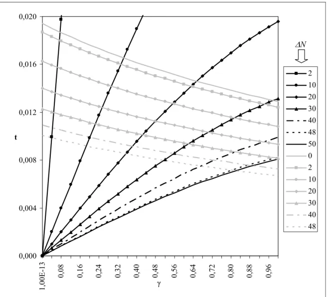
and (33) for ∆N =50, we can define the full set of equilibria for the location of downstream firms. In the following figure, these upper borders and the equilibrium curves for ∆N∈[ ]
0;50 are presented. The segments of the equilibrium curves above their intersections with the corresponding upper borders of the space of parameters will be ignored, since the boundary conditions0 ; ; ; * * *
* >
jb ja ib ia q q q
q do not hold simultaneously: [Insert figure 1]
In the previous figure, the equilibrium curve for ∆N =0 is not presented because when we have the same number of downstream firms located in both regions, which means that
0
=
for ∆N =50, which is defined by the curve t=2 3 according to equation (23), is not presented because of the scale of the chart.
Based on the chart of the previous figure, it is possible, through the positions of the equilibrium curves plotted from different values of ∆N, to see the results of the model obtained in section 2.2.3.1, in which we noted how the equilibrium level ∆N changes due to variations in parameters t and γ , in the interval ∆N∈
[
0;N)
. It can be observed that, for constant values of the transport cost t, as γ increases, the value of ∆N also increases, which means that an incentive is created for the migration of downstream firms from region B to region A. This graphical result is in accordance with the analytical model, which defined in section 2.2.3.1 that:( )
0
> ∂
∆ ∂
γ
N
; always
Intuitively, this mathematical result can be interpreted in the following manner: since the final consumer markets in both regions A and B are symmetrical, when there is an increase in the value of parameter γ (and consequently, in the transport cost of the input) and while the other conditions affecting the economy are kept unchanged, the downstream firms are affected by a force attracting them to region A. This occurs because, although the upstream firm is responsible for the transport of the input, when γ increases, this growth affects the input price charged to the downstream firms located in region B, according to equation (14), while the input price charged to downstream firms located in region A remains unchanged, according to equation (13). Another way to see this analysis is through equations (24) and (25), which represent the profit functions of the typical firms i∈A and j∈B. These are repeated below:
(
)(
)
[
]
{
}
{
[
(
)(
)
]
}
(
)
22 2
1 16
2 3
2 2
1 2
+
− ∆ − + − + + ∆ − + + =
N
N N t N
N t d
i
γ γ
π
In the previous equation, we can see that if γ increases, with all the rest remaining unchanged, both terms
{
2+t[
1+(
N−∆N)(
γ +2)
]
}
2 and{
2−t[
3+(
N−∆N)(
2−γ)
]
}
2 also increase, which means that the profit of the typical firms i∈A increases. For the typical firmsB
j∈ , the inverse holds true, as can be seen through their profit function:
(
) (
)(
)
[
]
{
}
{
[
(
) (
)(
)
]
}
(
)
22 2
1 16
2 2 1 2 2
2 3 2
+
∆ + − + − + + + ∆ + + + − =
N
N N t
N N t
d j
γ γ
γ γ
π
In the previous equation, when γ increases, with all the rest remaining unchanged, both terms
(
) (
)(
)
[
]
{
}
22 2
3
2−t + γ + N+∆N γ + and
{
2+t[
(
1−2γ) (
+ 2−γ)(
N+∆N)
]
}
2 decrease, leading to a fall in profits.( )
[
)
N N t
t N
; 0 ;
; ;
0 ∀ ∀ ∆ ∈
< ∂ ∆
∂ γ
Intuitively, this mathematical result is more complicated to interpret than the previous one because variations in parameter t are associated with two opposing effects, one of them being a force attracting firms to region A and the other a force attracting firms to region B. Increases in parameter t are reflected in an increase in the transport cost of the input, creating a force that attracts the downstream firms to region A, where the upstream firm is located. On the other hand, an incentive is also created for the dispersion of downstream firms in order to reduce competition and locate close to the local final consumers. Particularly in this model, where there are always more downstream firms in region A than in region B, the incentive to reduce competition is an ever-present reality. The overall effect of these two opposing forces, according to the chart and the analytical model, is that the incentive to reduce competition is stronger than the incentive for agglomeration in one region. One issue that should be highlighted in this result is that, in contrast to the work of MAYER (2000), in the analysis of the trade-off between the minimization of the production cost and the maximization of accessibility to final consumers, the downstream firms give more importance to the latter. A possible explanation for this is that MAYER (2000) only considered a duopoly in his model and the competition effect that favours dispersion was not as apparent as in this generalized model with N firms. The results of our model are in line with VENABLES (1996), where a very high trade cost led to a unique and stable equilibrium, characterized by the dispersion of downstream firms.
4 – Conclusion
References
AMITI, M., (2001), “Regional specialization and technological leapfrogging”, Journal of Regional Science, vol. 41, pp. 149-172.
BELLEFLAMME, P., TOULEMONDE, E., (2003), “Product differentiation in successive vertical oligopolies”, Canadian Journal of Economics, vol. 36, pp. 523-545.
FUJITA, M., HAMAGUCHI, N., (2001), “Intermediate goods and the spatial structure of an economy”, Regional Science and Urban Economics, vol. 31, pp. 79-109.
FUJITA, M., THISSE, J.F., (2002), Economics of Agglomeration – Cities, Industrial Location and Regional Growth. Cambridge, Cambridge University Press.
MARSHALL, A., (1920), Principles of Economics. London, Macmillan.
MAYER, T., (2000), “Spatial Cournot competition and heterogeneous production costs across locations”, Regional Science and Urban Economics, vol. 30, pp. 325-352.
PONTES, J.P., (2003), “Industrial clusters and peripheral areas”, Environment and Planning A, vol. 35, pp. 2053-2068.
PONTES, J.P., (2005), “Agglomeration in a vertically related oligopoly”, Portuguese Economic Journal, forthcoming.
VENABLES, A.J., (1996), “Equilibrium locations of vertically linked industries”,
0,000 0,004 0,008 0,012 0,016 0,020
1
,00E
-13
0,0
8
0,1
6
0,2
4
0,3
2
0,4
0
0,4
8
0,5
6
0,6
4
0,7
2
0,8
0
0,8
8
0,9
6
γ t
2
10
20 30
40
48 50
0
2 10
20
30 40
48
Figure 1 – Equilibrium of location curves (black) and upper borders of the space of parameters (grey) where all fifty downstream firms are producing for both regions, according to different values of ∆N.