A Work Project presented as part of the requirements for the award of a master’s degree in finance from NOVA – School of Business and Economics – and a master’s degree in Economics from Insper.
Firm-level political uncertainty and corporate financial policies
Daniel Strozzi Soares 39595
A project carried out on the Double Degree Program between Nova and Insper, under the supervision of:
Adriana Bruscato Bortoluzzo and Irem Demirci
Firm-level political uncertainty and corporate financial policies Abstract
Political events across countries have significant effects on corporate financial policies. Literature suggest that not only aggregate political uncertainty matters, but also at the firm level. Political risk indexes and data from public firms in the U.S. between 2002 and 2019 resulting in 117,049 firm-quarter observations are employed in empirical estimations of investment and cash holdings as dependent variables. Results show that the effect of firm-level policy uncertainty on investment is sensitive to the statistical model and that cash holdings is positively correlated to firm-level political uncertainty.
Keywords: Political uncertainty, cash holdings, investment
Incerteza política ao nível da firma e políticas financeiras corporativas Resumo
Acontecimentos políticos em diferentes países têm efeito significativos em políticas financeiras corporativas. A literatura sugere que não somente a incerteza política agregada tem importância, mas também ao nível da firma. Índices de risco político e dados de empresas públicas nos Estados Unidos entre 2002 e 2019 resultando em 117.049 observações são utilizados para uma estimação de seus efeitos sobre investimento e disponibilidades como variáveis dependentes. Resultados demonstram que o risco político ao nível da firma é sensível ao modelo estatístico utilizado e que disponibilidades são positivamente correlacionadas com o risco político ao nível da firma.
1. Introduction
Political uncertainty has been documented as a source of relevant and heterogeneous outcomes throughout economies in the world. An empirical framework with international data from 48 countries shows that uncertainty around national elections has significant economic outcomes (Julio; Yook, 2012). In the U.S., political events happening in the country’s government and around the world as well are associated with uncertainty about the country’s future policy, as for example the U.S. government shutdown and fiscal cliff in 2013, the debt ceiling dispute, the euro crisis and still many others (Baker et al., 2016). Such sources of political uncertainty are related to corporate financial policies like investment and hiring according to those authors. Also, since most of the market value of firms is attributable to their options to invest and grow in the future (Dixit; Pindyck, 1994), the negative effect of uncertainty on investments may play a relevant role on managers’ value-maximizing corporate decisions.
Firms actions with regard to their investments, cash holdings and other financial policies are decided simultaneously. Julio and Yook (2012) find that political uncertainty is related to corporate financial policies, and specifically, the increase in political uncertainty around elections causes a decrease in investments and a similar amount increase in cash holdings. In a number of researches elections were used as a policy uncertainty measure related to effects on foreign direct investments (Julio; Yook, 2016), M&A activity (Bonaime et al., 2018), innovation (Bhattacharya et al., 2017), equity and debt issuances (Jens, 2017), initial public offerings (Colak et al., 2013) and corporate governance (Amore; Minichilli, 2016). Also, other authors find that political uncertainty affect capital structure through effects on the cost of long-term debt and hence on other related corporate strategies as well (Bradley et al., 2016).
A three-component Economic Policy Uncertainty index (EPU) was developed by Baker et al. (2016), circumventing the generally timed characteristic of elections and producing a monthly-available source of data. The index is based on citations of determined keywords related to political uncertainty in newspapers, the present value of the effect of future scheduled tax code changes and disagreement among professionals over government purchases and consumer prices. According to their research, the index captures more information over aggregate risks related to politics or policy than only the ones generated by election-related uncertainties. It is negatively correlated with corporate investment, which is significantly stronger for firms with higher degree of investment irreversibility and more dependent on government spending (Gulen; Ion, 2016).
Other sources of risk are as well related to corporate financial policies. While some of the literature does not make distinction between the effects of systematic and idiosyncratic risk on investment, Panousi and Papanikolaou (2012) report that firm’s idiosyncratic and systematic stock-return risk affect corporate investment differently. Their results suggest a negative relationship between systematic risk and investment, but that might be altered depending on the quality of the proxy for investment opportunities, and a negative relationship between idiosyncratic risk, which is exacerbated by higher managerial risk aversion. Idiosyncratic risk is also documented to affect cash holdings, according to Bates et al. (2009). The authors provide evidence that the level of cash holdings in U.S. companies has changed in response to changes in firm characteristics from 1980 to 2016, being the increase in the average cash ratio less than 50% for firm in industries that experience the smallest increase in risk in the same period and almost 300% for firms in industries with the largest increase in risk.
Although the effect of aggregate political uncertainty on investment and other firm policies has been extensively demonstrated, not much is known about the consequences of non-aggregate political risks on cash holdings. Hassan et al. (2019) developed a measure of political uncertainty at the firm level, which contains a large within-sector and within-time variation. Such variation demonstrates that, besides the time series variation in the firm’s political risk, its position in the within-time and within-sector cross-section of the firm-level political risk might be as well relevant for managerial decision-making. Such concerns motivate the objective of this research.
This work’s objective is to understand the effects of firm-level and aggregate political uncertainty on the financial policies of public firm in the U.S. between 2002 and 2019. Specifically, the first tested hypothesis is that an increase in political risk causes a reduction in investment and the second tested hypothesis is that an increase in political risk causes an increase in cash holdings. Both firm-level and the aggregate risk measures, PRisk and EPU respectively, are used as proxies for political risk in all regressions, except when indicated otherwise. The first regression replicates Hassan et al. (2019)’s core regression, employing ordinary least squares regression (OLS) and firm size as the only control variable to regress investment on PRisk. Other regressions include control variables suggested by the literature and alternative model specifications to enhance causality claims in the empirical estimations. The magnitude of the effect of PRisk on investment is later compared to its magnitude on cash holdings and provides supporting evidence of how much of the change in cash holdings may be caused by PRisk due to
its effect on investment. Additionally, results show that the inclusion of control variables drive out little of the explanatory power of PRisk in the OLS specification, but in random and in fixed effects specifications, the explanatory power of PRisk is not statistically or economically significant. For the second hypothesis test, the predictions of Bates et al. (2009) that indicate an increase in cash holdings in response to increased risk are followed as supporting evidence. There is recognizably some degree of disagreement over the direction of the effect of political risk on cash holdings in the literature: while there is evidence that political uncertainty around elections, when firms cannot assess intentions from newly elected government officials, causes firms to hold less cash (Xu et al., 2016), there is also evidence in favor of the tendency for firms to save cash as a response to increased uncertainty due to the precautionary motive (Bates et al., 2009)1 or simply due to the retention of cash related to delayed investments (Julio; Yook, 2012). Similarly, financially constrained firms could store cash to offset borrowing constraints to future investments (Acharya et al., 2007). Although Bates et al. (2009) research general risk, and not specifically political risk, this work’s presumption of a positive correlation between cash and political uncertainty is supported on their results due to the similarity between the employed empirical strategies of both researches. The estimates provide evidence of a consistently positive effect of firm-level political risk on cash holdings, ranging from 0.53 % to 2.3% at the sample-mean cash ratio.
One concern over such empirical designs is the endogeneity in risk and corporate outcomes, as an increase in risk may itself be caused by increases in leverage. Hassan et al. (2019) argue for the exogeneity and causality of the firm-level political risk measure, which captures exogenous variations in risk caused by the political system itself, alleviating such concerns. Additionally, regression specifications using lagged variables and dynamic panels with lagged dependent variables are tested in order to address endogeneity concerns and enhance the set of evidence supporting causality. Specifically, the main cash holdings regression is reestimated using the three-period lagged correspondents of PRisk and EPU, due to their stronger correlation with cash holdings than with their one-period counterpart. A second alternative substitutes PRisk by a variable intended to capture longer periods of high political risk, denominated PRiskLT. The effect
of PRisk on cash is highest three periods after its incidence. Also, the effect accumulates and is stronger for firms facing longer periods of political risk. Finally, Arellano-Bond’s dynamic panel estimators (Arellano; Bond, 1991) are employed to reestimate investment and cash holdings as
function of the political risk measures and the control variables. In order to address endogeneity concerns, the models include the lagged values of the dependent variables and PRisk as instruments. Whereas the coefficient estimates of PRisk are sensitive to the models, the estimates confirm EPU’s negative effect on investment and PRiskLT’s strong positive effect on cash.
This proposal contributes to the lines of research in political uncertainty and corporate financial policy by testing hypotheses that idiosyncratic and systematic political risk affect investments and cash holdings. The effect on the latter variable has not been completely explored in the literature, so this work contributes with further discussion and econometric evidence. Also, alternative regression models are employed to circumvent endogeneity and enhance the causality of the political risk measures on investment and cash holdings. Their results bring new information about the relationship between the variables. Third, much of the literature does not make distinctions between the effects of aggregate and specific political risks. Hence, this research augments the evidence in the literature by complementing with such analysis. Lastly, datasets constructed from automated textual analysis and other big data sources are becoming increasingly important. This research develops on the use of such data.
The work is organized in the following four sections: section 2 reviews related literature. Section 3 describes the data. Section 4 presents the methodology for the empirical estimations and their results and discussion considering the related literature. Section 5 concludes.
2. Literature review
Cukierman (1980) and Bernanke (1983) present a theoretical framework where, under irreversible upfront investment costs2, the increased uncertainty about future payoffs to the investment increases the value of information about such outcomes, consequently inducing firms to delay investments (or temporarily decrease) to learn more about the future and make more profitable decisions. The latter author argues that the negative effect of uncertainty on investments is channeled through the larger probabilities of negative outcomes, what is not offset by potential good outcomes. Also, the uncertainty is interpreted in the model as the source of macroeconomic fluctuation on investment.
2 Dixit & Pindyck (1994) develop the idea of “Real Options Approach to Investment”, where investment decisions
are similar to exercising an financial option and have three characteristics: the investment has an upfront cost that is partially or completely irreversible; there is uncertainty over future returns; and there is a leeway about timing, in the sense that actions can be postponed to gather more information about future rewards (but not complete certainty).
More recent literature reports both theoretical models and empirical evidence of the effects of uncertainty on investments. Bloom et al. (2007), using firm-level data of U.K. manufacturing companies, shows that firms facing higher uncertainty (measured by a proxy for total firm-level risk) tend to have a weaker response of investment to demand shocks. The authors label such response as a “cautionary motive” that is similar to the real options approach of Dixit and Pindyck (1994): the option to wait for uncertainties to be solved is more valuable for firms facing higher uncertainty, what depresses investment responses largely in the short-run, but can also last up to 10 years into the future in the authors’ empirical tests. Bond and Cummins (2004) find similar results regarding the effect of uncertainty (total stock return volatility at firm-level) on investments of U.S. firms between 1982 and 1999. Panousi and Papanikolaou (2012) provide empirical evidence that both firm idiosyncratic and systematic risks are as well related to investment. Their results suggest a negative relationship between systematic risk and investment, but that might be altered depending on the quality of the proxy for investment opportunities, and a negative relationship between idiosyncratic risk, which is exacerbated by higher managerial risk aversion. Higher levels of institutional ownership attenuate the effect of managerial risk aversion on the risk-investment relationship.
Julio and Yook (2012) focus the discussion on the effects of political uncertainties derived from government policies or leadership on firm behavior. The potential endogeneity between political uncertainties and economic environment is a recognized challenge for the identification of causal effects, as economic downturns themselves may be the cause for political uncertainties. The authors’ identification strategy circumvents those issues by using the timing of elections as an indirect and exogenous measure of periods of higher political uncertainty. They argue that election years, due to their timed and recurring nature, cause exogenous shocks in political uncertainty and causes firms to delay investments “until the uncertainty related to future financial regulation and macroeconomic policy is resolved”. After controlling for other types of uncertainty, there is evidence that firms reduce investment as a response of higher political uncertainty, retaining roughly that same amount in cash holdings. A number of other authors have used elections as a policy uncertainty measure related to effects on foreign direct investments (Julio; Yook, 2016), M&A activity (Bonaime et al., 2018), innovation (Bhattacharya et al., 2017), equity and debt issuances (Jens, 2017), initial public offerings (Colak et al., 2013) and corporate governance (Amore; Minichilli, 2016).
In an approach to develop an index that captures overall political uncertainties across economies, Baker et al. (2016) developed a direct measure of Economic Policy Uncertainty (EPU), based on citations of determined keywords related to political uncertainty in newspapers. Such newspaper-based indices, according to them, have the advantage that they can be extended to many countries, backwards in time and disaggregated into subcategories. EPU is a country-wide index, being primarily based on the automated analysis of policy-related economic uncertainty coverage by major newspapers. In the U.S., 10 large newspapers are analyzed monthly, inside which articles containing the term “uncertainty” or “uncertain”, the terms “economic” or “economy” and one or more of the following terms: “congress”, “legislation”, “white house”, “regulation”, “federal reserve”, or “deficit”. Three other components of the index include the present value of future scheduled tax code expirations and the disagreement among professional forecasters over future government purchases and over consumer prices. Each of the components are normalized to their standard deviation and averaged using weights of 1/2 on the news-based component, and 1/6 on each of the three other components. Results from Baker et al. (2016) show that the EPU contains relevant distinct sources of variation compared to the traditional risk measure VIX. Also, it predicts delay on investments, but not uniformly in the cross-section of firms, rather being stronger for firms with higher degree of investment irreversibility and more dependent on government spending (Gulen; Ion, 2016).
Changes in investment policy caused by the shock in political uncertainty, or more specifically delay in investments, are associated with an increase in cash holdings (Julio and Yook, 2012). A consistent increase in cash holdings in U.S. firms between 1980 and 2006 was documented by Bates et al. (2009), who also summarize other four reasons why firms should hold cash. The first is the transaction motive: Firms face transaction costs when converting non-financial assets into cash necessary for payments. There are economies of scale related to these transaction costs, which is a reason large firm would hold less cash. Secondly, the precautionary motive suggests that firms hold cash in order to fund liquidity needs in adverse future states of nature where access to sources of funds are costly. Important evidence is found on the Acharya et al. (2007)’s model of cash-debt substitutability in the firm’s optimal decision. They suggest that both higher cash stocks and higher debt capacity (or negative debt) can enhance the firm’s ability to exercise investment opportunities. But in the presence of financial frictions and uncertain future cash flows, cash stocks and negative debt “perform different functions in the optimization of
investment under uncertainty” and are to be treated differently in the presence of frictions. In effect, financially constrained firms (identified by low correlation between cash flows and investment opportunities), who have a higher propensity to be credit-rationed in adverse states of nature, tend to allocate cash flows towards cash holdings instead of repayment of debt. The third one is the tax motive, which is related to higher costs for U.S. firms in repatriating foreign earnings, thus incentivizing such multinational firms to hold cash abroad. The fourth one is the agency motive, related to conflicts of interest between managers and shareholders. Firms that have entrenched managers or are headquartered in countries with higher agency problems tend to build excess cash stocks more intensively. Also, results from Fresard (2010) suggest that increases in cash holdings have significant benefits for firms, being related to market-share gains, better operating performance and higher market value.
Cash holdings are related to politics as well. Evidence from companies in China show that in the first year of a newly appointed city-government leader, whose actions cannot be foresighted by firms, thus causing political uncertainty, local companies hold less cash (Xu et al., 2016). According to the authors, the evidence supports a “grabbing hand hypothesis”, which suggests that firms expect a rent-seeking behavior from politicians. Thus, when a political turnover occurs, causing uncertainty, a firm perceives the situation as an opportunity for the newly appointed official to extract rents and that it is safer for the firm to hide its assets, especially the liquid ones like cash and equivalents. The firm will then reduce cash holdings in periods of such political uncertainty.
While some of the literature does not make distinction between the effects of systematic and idiosyncratic risk on investment, Panousi and Papanikolaou (2012) report that firm’s idiosyncratic and systematic stock-return risk affect corporate investment differently. More firm cash flow risk, which is idiosyncratic, is associated with larger increases in cash holdings (Bates et al. 2009). And the effect of firm-level cash flow risk on predicting cash holdings is substantially lower (more negative) than the effect of industry systematic cash flow risk, what indicates the importance of idiosyncratic risks to cash holdings.
Hassan et al. (2019) developed a measure of political uncertainty at the firm level (PRisk). It is a company-specific measure of political risk and represents the share of conference calls made by companies to the public in conjunction with earnings release that is devoted to topics related to politics. The share of the conversation is measured by counting the number of bigrams (two-word
terms) contained in conversations that are classified as words related to political risk according to an automated text analysis tool that learns the classification from a political training library. The count of each bigram is weighted by the relative frequency of that bigram on the training library, so that they adjusted to the fact that each passage may be more related to politics than others. According to its authors’ results, surprisingly, most part of the variation in political uncertainty across firms happens in the time variation for firms within the same sector. Contrasting the traditional view that uncertainty about political outcomes affect firms homogeneously, they show that variation of the aggregate political risk accounts for only 0.81% of the variation in their measure. Sector fixed-effects and the interaction sector and time fixed-effects account for 4.38% and 3.12%, respectively. 19.87% is explained by permanent differences across firms in a given sector and the largest part, 71.82%, at the firm-level and not explained by time or firm fixed effects. The authors’ result shows that this firm-level political uncertainty index correlates with some of the above-mentioned expected outcomes of risk, namely that it is negatively correlated with investment activity, positively with lobbying activity and others. The large within-sector and time variation in PRisk suggest that political risks differences in the level of risk between firms may have not only a relevant role at an aggregate level, but at the firm-level as well.
However, the discussion relating cash holdings and political uncertainty does not sufficiently describe the relation between the two variables, especially regarding idiosyncratic political risk. The firm-level political uncertainty has a strong idiosyncratic component (Hassan et al., 2019) as discussed earlier, which is related to other measures of risk and investment, but its relation to cash holdings was not explored in the literature. Still, models considering stable exposure of firms to aggregate political risk do not completely address the economic impacts of such risks.
3. Data
Datasets containing quarterly firm-level political risk data (PRisk) from public companies listed in the U.S. between 2002 and 2019 as measured by Hassan et al. (2019) and the Economic Policy Uncertainty index (EPU) for the U.S. (Baker et al., 2016) were used as measures of political risk. Each of the datasets are available at their respective authors’ website3. PRisk is a
company-specific measure of political risk. It represents the share of conference calls made by companies in
conjunction with earnings release that is devoted to topics related to politics. The share of the conversation is measured by counting the number of bigrams (two-word terms) contained in conversations that are classified as words related to political risk according to an automated text analysis tool that learns the classification from a political training library. The count of each bigram is weighted by the relative frequency of that bigram on the training library, so that they adjusted to the fact that each passage may be more related to politics than others. EPU is a country-wide index and follows a similar approach, being an index primarily based on the automated analysis of policy-related economic uncertainty coverage by major newspapers. In the U.S., 10 large newspapers are analyzed monthly, inside which articles containing the term “uncertainty” or “uncertain”, the terms “economic” or “economy” and one or more of the following terms: “congress”, “legislation”, “white house”, “regulation”, “federal reserve”, or “deficit”. Three other components of the index include the present value of future scheduled tax code expirations and the disagreement among professional forecasters over future government purchases and over consumer prices. Each of the components is normalized to their standard deviation and averaged using weights of 1/2 on the news-based component, and 1/6 on each of the three other components. Since the firm’s fiscal quarters may not end on the same months of the calendar quarter’s months, the monthly 4-component EPU index is calculated computing the average of the three months of the fiscal quarter ending on calendar quarter (Gulen; Ion, 2016), thus generating a small quarterly variation.
The quarterly data from companies’ financial statements (reported in U.S. dollars) comes from Wharton Research Data Services (WRDS) Compustat and are matched to the political risk data according to the gvkey identifier available in the sets. U.S. GDP growth comes from S&P Capital IQ. Restrictions to the time frame and listed companies are due to the availability and match of datasets. Observations from companies whose primary sectors are financials (SIC codes 6000 to 6799) and utilities (SIC codes 4900 to 4999) are then excluded, due to the capital requirements and/or other regulations complied by companies in these sectors, what could potentially mislead the effects intended to be studied in the empirical investigation. Observations are dropped when containing total assets or total revenue equal or below 0, total asset growth or total revenue growth above 100% and market capitalization below $ 10 million in 1971 dollars (roughly $ 62.4 million in 2019, according to inflation data from the U.S. Bureau of Labor Statistics, 2019), following Almeida et al. (2004).
Table 1 – Variable description
The table presents the description of all variables used in empirical estimations. The abbreviated reference in the literature for the definition of each variable is presented at the end of each description. The abbreviations correspond to the first letter of the authors’ last name: GI – Gulen and Ion (2016); BKS - Bates et al. (2009); HHLT - Hassan et al. (2019); BBD - Baker et al. (2016); PP - Panousi and Papanikolaou (2012); OPW - Opler et al. (1999).
Variable Description
Investment ratio (Inv) The ratio of capital expenditures to the previous quarter’s book value of total
assets (GI).
Cash holdings (CH) The ratio of cash and cash equivalents to the previous quarter’s book value
of total assets (BKS).
PRisk The logarithm of PRisk standardized by its sample standard deviation
(HHLT)
PRiskLT For each company, the average of the last eight quarters of PRisk. When less than eight quarters are available, the variable is treated as missing data.
EPU The monthly 4-component EPU index is averaged in three months of the
fiscal quarter ending on calendar quarter t, then the logarithm of the quarterly EPU is taken (BBD).
Market-to-book ratio (MtB)
Book value of total assets minus book value of equity plus market value of equity. The quarterly market value of equity is defined as the closing price times shares outstanding. The result is divided by book value of total assets (BKS).
Cash flow (CF) Cash flow scaled by the previous quarter’s book value of total assets (GI). Leverage ratio (Lev) The ratio of total debt to the previous quarter’s book value of total assets
(BKS).
Revenue growth (RG) The year on year growth of quarterly total revenue (GI).
Return (Ret) The logarithm of quarterly stock price closing over the previous quarter’s
closing price (PP).
Firm size (Size) Natural logarithm of total assets (BKS). Cash flow volatility
(CFV)
For each firm-quarter, the standard deviation of that firm’s cash flow using the whole preceding time series. At least twelve quarters of non-missing cash flow data are required (OPW).
Net working capital ratio (NWC)
Net working capital minus cash and cash equivalents. The result is scaled by the previous quarter’s book value of total assets (BKS).
R&D expenses ratio (RnD)
The ratio of research and development expenditures (R&D) to total revenue (BKS).
Cash acquisitions ratio (Acq)
The ratio of cash expenditures on M&A acquisitions to the previous quarter’s book value of total assets (BKS).
Dividend payout dummy (Div)
A dummy variable equal to one if the firm payed common or preferred dividends the quarter before (BKS).
Industry median cash flow volatility (IndCFVol)
For each firm-quarter, the standard deviation of that firm’s cash flow using the whole preceding time series is computed. The median cash flow for each quarter within the two-digit Standard Industry Classification (SIC) code is then computed. At least twelve quarters of non-missing cash flow data are required (BKS).
GDP growth (GDP) Year over year percentage change of quarterly U.S. real GDP (GI).
Since capital expenditures are reported accumulated along fiscal quarters within the same year, the values are adjusted to report quarter-specific expenditures. After the construction of the variable specifications, the 1 % largest and the 1 % lowest values from each firm-specific variable are truncated, so that the values below the 1st observation or above the 99th observation are set equal the nearest inward value to the cutoffs. This process known as winsorization helps avoiding potential misleading effects from outliers (Panousi and Papanikolaou, 2012). Observations containing missing data are not considered by the regression estimations. Table 1 details the construction of variables. Table 2 describes summary statistics of all explained and explanatory variables and Table 3 reports the correlation matrix. For an augmented Dickey-Fuller test for unit root processes, PRisk and EPU are averaged inside groups (firms) and treated as time series. The test of random walk with drift rejects the null hypothesis of unit root processes for both variables with p-values of 0.002 and 0.046, respectively. The inclusion of the drift term causes the test statistic to vary. For the sequence of the work, both variables are considered stationary.
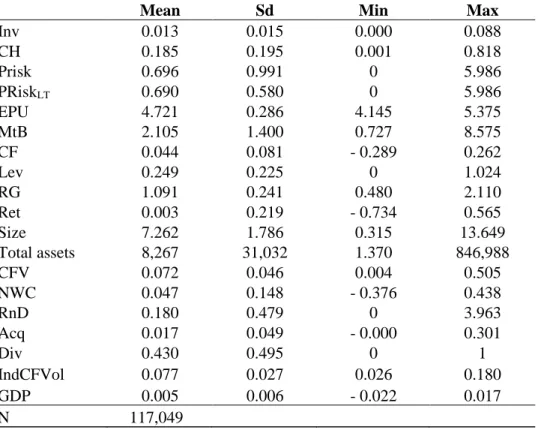
Table 2 –Summary statistics
The sample consists of nonutility and nonfinancial U.S. firms in WRDS Compustat from 2002 to 2019 for non-missing data, after the screening and data treatment described in section 2. The columns present variable averages (Mean) standard deviations (Sd), minimum (Min) and maximum (Max) values. Variable definitions are provided in Table 1, except for PRisk and PRiskLT which are reported not logarithmized.
Mean Sd Min Max
Inv 0.013 0.015 0.000 0.088 CH 0.185 0.195 0.001 0.818 Prisk 0.696 0.991 0 5.986 PRiskLT 0.690 0.580 0 5.986 EPU 4.721 0.286 4.145 5.375 MtB 2.105 1.400 0.727 8.575 CF 0.044 0.081 - 0.289 0.262 Lev 0.249 0.225 0 1.024 RG 1.091 0.241 0.480 2.110 Ret 0.003 0.219 - 0.734 0.565 Size 7.262 1.786 0.315 13.649 Total assets 8,267 31,032 1.370 846,988 CFV 0.072 0.046 0.004 0.505 NWC 0.047 0.148 - 0.376 0.438 RnD 0.180 0.479 0 3.963 Acq 0.017 0.049 - 0.000 0.301 Div 0.430 0.495 0 1 IndCFVol 0.077 0.027 0.026 0.180 GDP 0.005 0.006 - 0.022 0.017 N 117,049
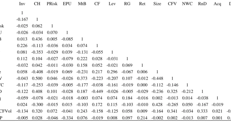
Table 3 - Correlation matrix
The sample consists of nonutility and nonfinancial U.S. firms in WRDS Compustat from 2002 to 2019 for non-missing data, after the screening and data treatment described in section 2. The table presents the correlation between the main explained and explanatory variables. Variable definitions are provided in the Table 1, except for PRisk, which is reported not logarithmized.
Inv CH PRisk EPU MtB CF Lev RG Ret Size CFV NWC RnD Acq Div
Inv 1 CH -0.167 1 PRisk -0.025 0.062 1 EPU -0.026 -0.034 0.070 1 MtB 0.013 0.436 0.005 -0.085 1 CF 0.226 -0.113 -0.036 0.034 0.074 1 Lev 0.081 -0.353 -0.029 0.039 -0.131 -0.055 1 RG 0.112 0.104 -0.027 -0.079 0.222 0.028 -0.031 1 Ret -0.032 0.042 -0.011 -0.030 0.158 0.052 -0.021 0.069 1 Size 0.058 -0.408 -0.019 0.069 -0.231 0.217 0.296 -0.067 0.006 1 CFV -0.043 0.500 0.046 -0.026 0.373 -0.223 -0.207 0.107 -0.012 -0.448 1 NWC -0.117 -0.253 -0.039 -0.005 -0.177 -0.038 -0.161 -0.019 0.000 -0.112 -0.146 1 RnD -0.122 0.408 0.101 -0.028 0.187 -0.449 -0.026 -0.005 -0.029 -0.236 0.325 -0.212 1 Acq -0.059 -0.078 -0.021 -0.018 -0.003 0.074 0.074 0.184 -0.016 0.002 -0.013 0.014 -0.038 1 Div 0.024 -0.300 -0.015 0.015 -0.103 0.172 0.115 -0.103 -0.010 0.428 -0.265 0.050 -0.167 -0.019 1 IndCFVol -0.134 0.320 0.072 -0.041 0.243 -0.158 -0.125 0.058 0.009 -0.164 0.341 -0.034 0.333 0.021 -0.128 GDP -0.005 0.028 -0.046 -0.334 0.076 -0.019 0.008 0.097 0.214 -0.002 0.002 -0.013 0.007 0.001 0.005 Source: author's own elaboration
4. Results 4.1. Investment
In order to learn about the behavior of the political risk variables PRisk and EPU, first the investment ratio is regressed on those variables and on literature-suggested controls. This first step is motivated by the fact that Hassan et al. (2019) report their results not including relevant controls suggested by the literature for the investment regression. Indeed, the authors regress the capital expenditures on PRisk, firm size, and sector and time fixed effects. For the purpose of this research, the following equation for investment is estimated:
𝐼𝑛𝑣𝑖,𝑡 = 𝛼𝐼+ 𝛽𝐼1𝑃𝑅𝑖𝑠𝑘𝑖,𝑡−1+ 𝛽𝐼2𝐸𝑃𝑈𝑖,𝑡−1+ 𝛿′𝑋𝐼𝑡−1+ 𝜀𝐼𝑖,𝑡 (1)
Where variables are indexed on firm i and in quarter t and Inv represent the investment ratio. Besides the two political risk measures, PRisk and EPU, the specification includes a constant (𝛼𝐼) and an unobserved error term (𝜀𝐼𝑖,𝑡). The vector of control variables 𝑋𝐼 include the
market-to-book ratio (MtB), Cash flow to assets ratio (CF), revenue growth (RG) and quarterly GDP growth (ΔGDP) (Gulen and Ion, 2016; Panousi and Papanikolaou, 2012), idiosyncratic risk (CFV), firm size (Size), firm’s stock return (Ret) and leverage ratio (Lev) (Panousi and Papanikolaou, 2012). Table 4 details the results of equation (1), reported in six different specifications, each one in one column, ranging from column (1), which simulates Hassan et al. (2019)’s specification (using an alternative variable construction however), to column (6), which is estimated using the within-estimator and including all controls and fixed effects.
Column (1) demonstrates the statistical significance of PRisk as an explanatory variable for investment. The coefficient suggests that, all else constant, the increase in PRisk by one standard deviation is associated with a decrease of 0.000267points in the investment to total assets ratio, representing a 2 % decrease in the ratio at the sample mean. Such results are larger than Hassan et al. (2019)’s, who found a 1.4 % decrease in the investment to assets ratio at their sample mean. One potential source of divergence lies on the method to construct the variables. Although both variables represent the capital investment to total assets, those authors construct the investment measure using a perpetual inventory method, which adds to the investment rate the previous-period inflated property, plant and equipment, discounted by a 10% depreciation rate.
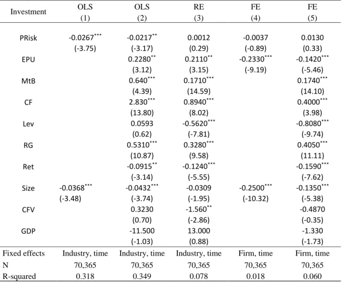
Table 4 – Political risk and investment
Coefficients are presented for each regression specification in hundred units and their respective t-statistic in parenthesis. The sample consists of nonutility and nonfinancial U.S. firms in WRDS Compustat from 2002 to 2019 for non-missing data, after the screening and data treatment described in section 2. Capital expenditures to total assets (Investment) is regressed on one-period lagged explanatory variables, using ordinary least squares (OLS), the random-effects estimator (RE) and the fixed-effects within estimator (FE), which are indicated at the top of the columns. Controls, industry and firm fixed effects are included gradually and are indicated at the bottom of the columns alongside with the adjusted R-squared and the size of the sample (N). Robust standard errors are clustered at the firm-level. Statistical significance at the 1%, 5% and 10% are denoted by ***, ** and * respectively.
Investment OLS OLS RE FE FE
(1) (2) (3) (4) (5) PRisk -0.0267*** -0.0217** 0.0012 -0.0037 0.0130 (-3.75) (-3.17) (0.29) (-0.89) (0.33) EPU 0.2280** 0.2110** -0.2330*** -0.1420*** (3.12) (3.15) (-9.19) (-5.46) MtB 0.640*** 0.1710*** 0.1740*** (4.39) (14.59) (14.10) CF 2.830*** 0.8940*** 0.4000*** (13.80) (8.02) (3.98) Lev 0.0593 -0.5620*** -0.8080*** (0.62) (-7.81) (-9.74) RG 0.5310*** 0.3280*** 0.4050*** (10.87) (9.58) (11.11) Ret -0.0915** -0.1240*** -0.1590*** (-3.14) (-5.55) (-7.62) Size -0.0368*** -0.0432*** -0.0309 -0.2500*** -0.1350*** (-3.48) (-3.74) (-1.95) (-10.32) (-5.38) CFV 0.3230 -1.560** -0.4870 (0.70) (-2.86) (-0.35) GDP -11.500 13.000 -1.330 (-1.03) (0.88) (-1.73)
Fixed effects Industry, time Industry, time Industry, time Firm, time Firm, time
N 70,365 70,365 70,365 70,365 70,365
R-squared 0.318 0.349 0.078 0.018 0.060
Source: author’s own elaboration
Most importantly, however, are the results obtained in the following regressions. Whereas that result is only slightly changed after the inclusion of controls to the OLS specification, shown in column (2), the regression specifications using RE and FE change the results more strongly, having PRisk completely lose its explanatory power in such models, as shown in columns (3) to (5). Given the relative smaller variance of PRisk across time when compared to its cross-section, documented by Hassan et al. (2019), it is possible that the fixed effects transformations eliminate
all its variation and explanatory power compared to OLS models. Wooldridge (2003) suggests that RE is generally more efficient than OLS and could be preferred to FE when estimating non-time-varying variables and if unobserved fixed effects are not correlated with explanatory variables. To circumvent this last issue, the author suggests the inclusion in the model of as many time-constant controls as possible. The inclusion of a set of controls suggested by different recognized works in the literature and the similar conclusion derived from both models point out that the lack of explanatory power of PRisk is not misled by characteristics of the models or endogeneity caused by the lack of controls. Another possible issue is that companies are slow to respond to increased PRisk by cutting capital expenditures, meaning that high PRisk is affecting companies’ investments in periods further in the future than in the next one. For such question, alternative regressions were tested (not reported) substituting the one-period lagged PRisk by the four-period lagged PRisk, which are similarly correlated with Inv4. Results are not changed.
On the other hand, EPU remains negatively and significantly correlated with investment in most of the cases, what is consistent with evidence in the literature (Baker et al., 2016; Gulen; Ion, 2016). But, since it is a country-aggregated measure, having variation between companies only due to differences in their respective fiscal-year end, fixed effects potentially blur its explanatory power. In any case, the distinction between EPU and PRisk is clear, corroborating results from Panousi and Papanikolaou (2012) that evidence the distinction between the effects of systematic and firm-specific (or idiosyncratic) risks on investments. The significance of the coefficients of CFV and GDP are driven out by the inclusion of industry and time fixed effects, suggesting that their effect (or variability) is absorbed by the fixed effects (which was expected for GDP), whereas the coefficients of Size, MtB, CF and Lev are consistent with the results obtained by Panousi and Papanikolaou (2012)5.
4.2. Cash holdings
The base cash holdings regression is estimated according to the following specification:
4 A correlation matrix is presented at the section 4.3. Due to the similarity of the results with the presented at Table
4, the alternative specification is not reported.
5 Panousi and Papanikolaou (2012) use the definition of ratio of book value of equity to book value of total assets as
leverage and obtain a positive coefficient on explaining investment. Since book equity + book liabilities (including debt) = total assets, keeping total assets constant, an equity and liabilities are inversely related. Thus, a measure of leverage using liabilities to total assets should be inversely related to investment.
𝐶𝐻𝑖,𝑡 = 𝛼𝐶+ 𝛽𝐶1𝑃𝑅𝑖𝑠𝑘𝑖,𝑡−1+ 𝛽𝐶2𝐸𝑃𝑈𝑡−1+ 𝛿′𝑋𝐶,𝑡−1+ 𝜀𝐶𝑖,𝑡 (2)
Where CH on the left-hand side of the equations represent the cash ratio. The specification of equation (2) and the inclusion of control variables in the vector 𝑋𝐶 follow the results of Opler et al. (1999) and Bates et al. (2009), who report determinants of cash holdings for firms in the U.S. The list of controls includes MtB, Size, CF, net working capital to assets ratio (NWC), capital expenditures to assets ratio (Inv), Lev, industry cash flow risk (ICF), dividend payout (Div), R&D expenditure to sales ratio (RnD) and cash acquisitions to assets ratio (Acq). The specification includes a constant (𝛼𝐶) and an unobserved error term (𝜀𝐶𝑖,𝑡) and is estimated using the fixed-effects (within-estimator) model. Errors are assumed to be potentially heteroskedastic in all specifications and robust standard errors are clustered at the firm level. Table 5 details the results of equation (2) reported in six different specifications, ranging from column (1), which does not include controls, to column (6), where the within-estimator is used and includes all suggested controls.
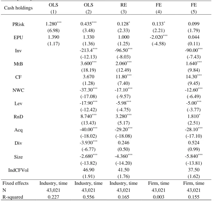
PRisk is consistently positively correlated with CH across all specifications. The magnitude of the coefficients of the PRisk variable suggest that, all else constant, one standard deviation increase in PRisk is associated with an average increase in the ratio of cash holdings to total assets ranging from around 0.001 to 0.00435 percentage points, representing an average increase ranging from 0.53 % to 2.3 % at the mean cash ratio for the sample. If all companies in the sample were subject to one standard deviation increase in PRisk, it would represent a U$ 546 million to U$ 2.371 million total increase in the cash and short-term investments of those companies. Given that investments are among the included controls, such effect of PRisk on CH is potentially additional to the increase in CH as consequence of delayed investments, reported by Julio and Yook (2012). Also, the range of variation of PRisk in the sample (after treatment) is around 6 standard deviations, indicating that a variation of roughly 12.5 % around the mean CH may possibly occur due to variations in PRisk. Column (3) and (5) show that in the RE and FE regressions including controls, its explanatory power is weak or not statistically significant although consistently positive.
Table 5 – Political risk and cash holdings
Coefficients are presented for each regression specification in hundred units and their respective t-statistic in parenthesis. The sample consists of nonutility and nonfinancial U.S. firms in WRDS Compustat from 2002 to 2019 for non-missing data, after the screening and data treatment described in section 2. Cash and equivalents to total assets (CH) is regressed on one-period lagged explanatory variables, using ordinary least squares (OLS), the random-effects estimator (RE) and the fixed-effects within estimator (FE), which are indicated at the top of the columns. Controls, industry and firm fixed effects are included gradually and are indicated at the bottom of the columns alongside with adjusted R-squared and the size of the sample (N). Robust standard errors are clustered at the firm-level. Statistical significance at the 1%, 5% and 10% are denoted by ***, ** and * respectively.
Cash holdings OLS OLS RE FE FE
(1) (2) (3) (4) (5) PRisk 1.280*** 0.435*** 0.128* 0.133* 0.099 (6.98) (3.48) (2.33) (2.21) (1.79) EPU 1.390 1.330 1.000 -2.020*** 0.044 (1.17) (1.36) (1.25) (-4.58) (0.11) Inv -213.4*** -96.50*** -90.00*** (-12.13) (-8.03) (-7.43) MtB 3.600*** 2.060*** 1.640*** (18.19) (12.49) (9.84) CF 3.670 11.80*** 14.30*** (1.28) (7.40) (9.45) NWC -37.30*** -17.10*** -12.60*** (-17.08) (-9.57) (-6.49) Lev -17.90*** -5.98*** -5.00*** (-12.42) (-4.75) (-3.77) RnD 8.740*** 3.280*** 1.810* (13.43) (5.17) (2.51) Acq -40.00*** -29.20*** -28.10*** (-18.02) (-18.08) (-17.10) Div -3.930*** 0.246 0.524 (-6.77) (0.50) (0.99) Size -2.680*** -4.360*** -5.840*** (-13.82) (-14.20) (-13.81) IndCFVol 46.90 41.50 37.50 (1.91) (1.76) (1.62)
Fixed effects Industry, time Industry, time Industry, time Firm, time Firm, time
N 43,021 43,021 43,021 43,021 43,021
R-squared 0.227 0.556 0.165 0.003 0.155
Source: author’s own elaboration
The evidence of a positive correlation between political risk and cash is supported by explanations documented by Bates et al. (2009), including that managers tend to hold more cash as precaution in anticipation of challenging periods ahead. For Xu et al. (2016)’s test of a response of corporate cash holdings to general uncertainty related to elections, the correlation between cash
and political uncertainty is generally negative. Their conclusion points to the fact that companies anticipate the rent-seeking behavior of newly appointed government officials and reduce liquid assets, such as cash, in an attempt to protect their assets from such behavior. Given the nature of the PRisk measure that captures political uncertainty not only related to newly elected officials, its positive correlation with cash holdings is more closely explained by the description of Bates et al. (2009). Those authors also suggest a general increase in the cash holdings of U.S. firms in the last decades due to the change in firms’ characteristics that explain the variation in their balance sheet cash. The previously presented results may add to their conclusion by confirming that political risk is one of the to-be-considered variables.
For EPU, where no controls are included column (4), its sign suggest a negative correlation of aggregate political uncertainty with CH. After the inclusion of controls, however, its statistical significance is driven out, suggesting that its effect on cash holdings may only work through indirect channels like capital or research and development expenditures.
Also interestingly, the coefficient of Inv is very large, roughly 7.5 and 3.5 times larger than magnitudes found by Bates et al. (2009), for OLS and FE specifications, respectively. The magnitudes indicate that, all else constant, for each additional unit of capital expenditures, the companies’ cash ratio decreases on average from 0.9 to 2.0 units. The sign of coefficients on MtB, Size, NWC, Lev, Acq are similar to those obtained by Bates et al. (2009). Div and RnD similar for the OLS specifications, whereas CF varies, but generally having low statistical significance. Also, Bates et al. (2009) find adjusted R-squared values of 0.455 and 0.154 for OLS and FE estimates, respectively, compared to 0.556 and 0.155 obtained for the similar regressions shown at the columns (2) and (5).
4.3. Long-term effect of political uncertainty
In order to test the potential effect of PRisk in corporate variables in periods further than one period, alternative specifications of regression (1) and (2) are tested. First, a correlation matrix between the dependent variables is constructed to select the lagged periods that are more strongly correlated with the dependent variables. Results for up to four periods are shown in Table 6.
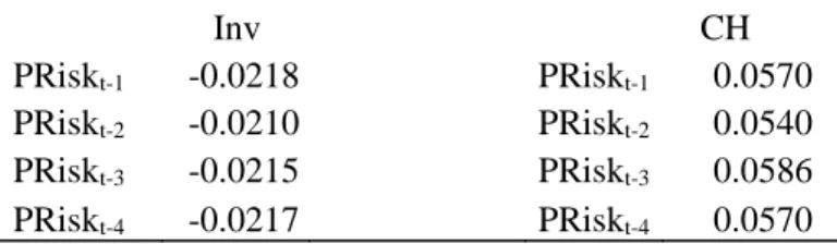
The first lagged period of PRisk has the strongest correlation with investment and the third lagged period in the case of CH. An alternative test (not reported), where quarterly averages of all firms for Inv and CH are correlated with average PRisk between firms, simulating a time series,
suggests similar results for the strongest correlation. In the second step, even though only the correlation of PRisk with CH is the strongest for the three-period lagged variable, both PRisk and EPU are replaced by their three-period similar, whose results are reported at the columns (1) and (2) of Table 7. In fact, as mentioned before, the results for the investment regression are not changed by such modification, thus only the results of the cash holdings regression are reported. Controls are not reported due to their similarity to previously reported specifications.
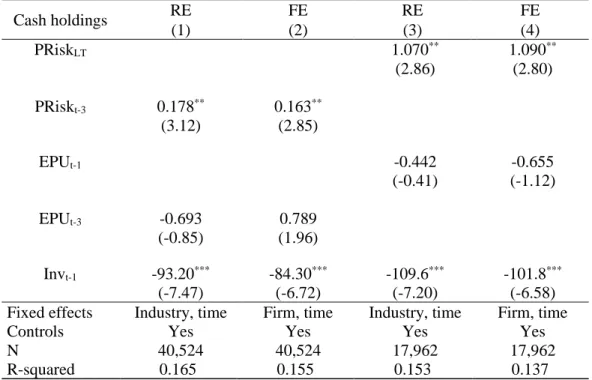
A stronger correlation of the three-period lagged PRisk correlation with cash holdings is confirmed at both estimates when compared to estimates in the previous section. Being the political risk in quarter t more strongly correlated with higher cash holdings in quarter t+3 suggests that such political risks are indeed identified, since they have been discussed in quarter t results conference, but their consequences are mostly identifiable only after three quarters. The magnitude of the coefficient of PRiskt-3 suggest that, all else constant, an increase of one standard deviation
in PRisk is associated with an increase of 0.00163 units, or 0.87 % , in the cash ratio at the sample mean.
Table 6 - Correlation matrix between dependent variables and lagged PRisk
The sample consists of nonutility and nonfinancial U.S. firms in WRDS Compustat from 2002 to 2019 for non-missing data, after the screening and data treatment described in section 2. The table presents the correlation matrix between the ratio of cash and equivalents to total assets, PRisk and its lagged specifications. Variable definitions are provided in Table 1.
Inv CH
PRiskt-1 -0.0218 PRiskt-1 0.0570 PRiskt-2 -0.0210 PRiskt-2 0.0540 PRiskt-3 -0.0215 PRiskt-3 0.0586 PRiskt-4 -0.0217 PRiskt-4 0.0570
Source: author’s own elaboration
Columns (3) and (4) of Table 7 shows again an alternative of regression (2), where PRisk is replaced by a measure intended to capture its long-term effect denominated as PRiskLT. This
measure represents, for each firm, the average of the last eight quarters of PRisk (after treatment, as described in Table 1). When less than eight quarters of PRisk are available, the variable is treated as missing data. The coefficient of PRiskLT, shown in column (3), is statistically significant and
roughly 6 times larger than its one-period differenced counterpart. The larger estimate reinforces the evidence that political risk affects corporate financial policies for periods into the future, rather
than only instantly. Also, the result points out that the effects of longer exposures to risk on cash holdings may accumulate across time and become stronger. Despite having evidently absorbed the time effects of political risk on CH, the FE regression using PRiskLT as regressor in column (4)
depicts a more significant effect of long-term exposures to political risk, when compared to the results discussed in the previous section.
Table 7 – Alternative lagged variables
Coefficients are presented for each regression specification in hundred units and their respective t-statistic in parentheses. The sample consists of nonutility and nonfinancial U.S. firms in WRDS Compustat from 2002 to 2019 for non-missing data, after the screening and data treatment described in section 2. In columns (1) and (2) cash holdings are estimated as the dependent variable regressed on three-period lagged PRisk (PRiskt-3) and EPU (EPUt-3) and one-period lagged controls. In columns (3) and (4) PRiskt-3 is replaced by PRiskLT and EPUt-1 is used as usual. Random (RE) or fixed (FE) effects specifications are indicated at the top of the columns. All regressions include the controls as discussed in section 3. The presence of fixed effects is indicated at the bottom of the columns alongside with the size of the sample (N). Robust standard errors are clustered at the firm-level. Statistical significance at the 1%, 5% and 10% are denoted by ***, ** and * respectively. Cash holdings RE FE RE FE (1) (2) (3) (4) PRiskLT 1.070** 1.090** (2.86) (2.80) PRiskt-3 0.178** 0.163** (3.12) (2.85) EPUt-1 -0.442 -0.655 (-0.41) (-1.12) EPUt-3 -0.693 0.789 (-0.85) (1.96) Invt-1 -93.20*** -84.30*** -109.6*** -101.8*** (-7.47) (-6.72) (-7.20) (-6.58)
Fixed effects Industry, time Firm, time Industry, time Firm, time
Controls Yes Yes Yes Yes
N 40,524 40,524 17,962 17,962
R-squared 0.165 0.155 0.153 0.137
Source: author’s own elaboration
The results support the conclusion that not only the action of institutions doing policy affects companies, but the uncertainty surrounding those decisions as well. As Gulen and Ion (2016) point out, the damage of policy uncertainty when making policy decisions might be as harmful as making a wrong decision, what indicates that regulators should take that effect into account. Similarly, Bhattacharya et al. (2017) find that policy uncertainty has greater effects on innovation than the policy itself.
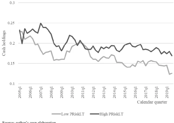
Figure 1 illustrates the average behavior of firms facing long periods of high political risk by showing the average quarterly cash ratio of firms with PRiskLT above median, denoted by “High
PRiskLT”, against firms with PRiskLT below median, denoted by “Low PRiskLT”. Firms sorted by
a conservative cutoff of high PRiskLT present consistently higher levels of cash holdings, with the
exception of the first quarters of the sample and the quarters 2010q2 through 2011q2.
Figure 1 – Quarterly average cash ratio by levels of PRiskLT
The graph shows the quarterly average cash to total assets ratio (cash holdings) for firms having PRiskLT below median in light gray against firms having PRiskLT above median in dark gray. Average cash holdings is computed considering all firms below or above the total-sample median PRiskLT for each quarter. The sample consists of nonutility and nonfinancial U.S. firms in WRDS Compustat from 2002 to 2019 for non-missing data, after the screening and data treatment described in section 2.
Source: author’s own elaboration
4.4. Dynamic panels
Arellano-Bond’s (Arellano; Bond, 1991) dynamic panel GMM estimators are used to estimate the investment and cash holdings equations (1) and (2) and their results are reported in Table 8. Besides the model’s standard specification that includes lags of the dependent variable as its instruments, the regressions reported at the table below use lags of PRisk as their instruments to circumvent the possibility that PRisk is endogenous in the model.
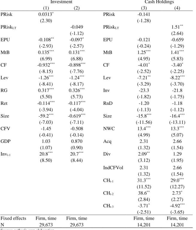
Table 8 – Dynamic panels of investment and cash holdings
Coefficients are presented for each regression specification in hundred units and their respective t-statistic in parentheses. The sample consists of nonutility and nonfinancial U.S. firms in WRDS Compustat from 2002 to 2019 for non-missing data, after the screening and data treatment described in section 2. Capital expenditures to total assets (Investment) and cash and equivalents to total assets (Cash Holdings) as the dependent variable are regressed on controls as discussed in the section 3. Columns (2) and (4) replace PRisk for PRiskLT. Additionally, lagged variants of the dependent variables, PRisk and PRiskLT are used as their instruments in all regressions. The presence of fixed effects is indicated at the bottom of the columns alongside with the size of the sample (N). Robust standard errors are clustered at the firm-level. Statistical significance at the 1%, 5% and 10% are denoted by ***, ** and * respectively.
Investment Cash Holdings
(1) (2) (3) (4) PRisk 0.0313* PRisk -0.141 (2.30) (-1.28) PRiskLT -0.049 PRiskLT 1.51** (-1.12) (2.64) EPU -0.108** -0.097* EPU -0.121 -0.659 (-2.93) (-2.57) (-0.24) (-1.29) MtB 0.135*** 0.131*** MtB 1.25*** 1.41*** (6.99) (6.88) (4.95) (5.83) CF -0.932*** -0.898*** CF -4.01* -3.40* (-8.15) (-7.76) (-2.52) (-2.25) Lev -1.26*** -1.24*** Lev -7.21** -8.22*** (-8.41) (-8.17) (-3.29) (-3.70) RG 0.317*** 0.326*** Inv -23.3 -21.8 (5.50) (5.73) (-1.82) (-1.75) Ret -0.114*** -0.117*** RnD -1.20 -1.18 (-3.94) (-4.04) (-1.13) (-1.12) Size -59.2*** -0.619*** Size -15.8*** -16.4*** (-7.03) (-7.11) (-11.56) (-13.11) CFV -1.45 -0.508 NWC 13.4*** 13.3*** (-0.41) (-0.14) (4.99) (5.07) GDP 1.03 0.870 Acq 2.31 2.66 (1.07) (0.90) (1.32) (1.54) Invt-1 20.8*** 20.7*** Div 2.09** 1.29 (8.50) (8.44) (3.12) (1.95) IndCFVol 2.31 2.66 (1.32) (1.54) CHt-1 31.3*** 29.0*** (11.52) (12.27) CHt-2 38.6** 2.73* (2.84) (2.27) CHt-3 -3.71* -4.92*** (-2.51) (-3.65) Fixed effects Firm, time Firm, time Firm, time Firm, time
N 29,673 29,673 14,201 14,201
The lag structure of instruments is selected based on the order of the serial correlation of the first-differenced errors, indicated by Arellano-Bond’s postestimation test, since no second-order (or higher) serial correlation in the first-differenced errors is an indication of the validity of the estimator’s condition of no serial correlation in the structure of errors (Roodman, 2009). Lemmon et al. (2008), researching capital structure models, suggest that serial correlation in the error structure might be present in cases where financial adjustment is costly, economic shocks are persistent or autocorrelated independent variables are omitted from the specification. Thus, the models are estimated using the least number of lags possible to satisfy that condition, which is one lag for the investment regression and three lags for the cash holdings regression.
Column (1) shows that PRisk has weakly significant effect, whereas EPU is confirmed as negatively correlated with investment in both regressions of columns (1) and (2). Generally, coefficients of other control variables slightly change their magnitude when compared to the regressions reported previously. Most remarkably is the coefficient on CF, which was previously consistently positively correlated with investments, but has now the opposite estimate. The negative correlation contradicts results from Gulen and Ion (2016), who found a strong positive correlation between cash flow and investments.
For the cash holdings regressions, shown in columns (3), PRisk and Inv, which were previously strongly correlated with CH, are now not statistically distinguishable from zero. However, PRiskLT coefficient shown in column (4) confirm its strong positive effect on CH,
supporting that similar conclusion on the previous section.
5. Conclusion
Political events or decisions made by political leadership have consequences to companies and the economic environment. Uncertainty surrounding those events and decisions are possibly as well important or even more influential, as the conclusion of Bhattacharya et al. (2017) that policy uncertainty affects a country’s innovation activities more than policy itself does. This work provides evidence that the companies’ most liquid assets, cash and short-term investments, are positively affected by political uncertainty at the firm-level even after controlling for other relevant variables, like investments, which is depressed in times of high political uncertainty and tend to cause an increase cash. Aggregate political uncertainty is demonstrated to affect corporate
financial policies at different directions as the firm-level measure does. Effects of firm-level political uncertainty may be the strongest not at the same period of its incidence, but most possibly at further periods in the future. Lastly, databases derived from automated text analysis contain relevant information about the financial behavior of companies.
References
ACHARYA, V. V.; ALMEIDA, H.; CAMPELLO, M. Is cash negative debt? A hedging perspective on corporate financial policies. Journal of Financial Intermediation, v. 16, n. 4, p. 515–554, 2007.
ALMEIDA, H.; CAMPELLO, M.; WEISBACH, M. S. The Cash Flow Sensitivity of Cash. The
Journal of Finance, v. 59, n. 4, p. 1777–1804, 2004.
AMORE, M. D.; MINICHILLI, A. Local political uncertainty, family control and investment behavior. Journal of Financial and Quantitative Analysis, v. 53, n. 4, p. 1781–1804, 2018. ARELLANO, M.; BOND, S. Some tests of specification for panel data: Monte carlo evidence and an application to employment equations. Review of Economic Studies, v. 58, n. 2, p. 277–297, 1991.
BAKER, S. R.; BLOOM, N.; DAVIS, S. J. Measuring economic policy uncertainty. The
Quarterly Journal of Economics, v. 131, n. 4, p. 0–52, 2016.
BATES, T. W.; KAHLE, K. M.; STULZ, R. M. Why do U.S. firms hold so much more cash than they used to? The Journal of Finance, v. 64, n. 5, p. 1985–2021, 2009.
BERNANKE, B. S. Irreversibilities, uncertainty, and cyclical investment. The Quarterly Journal
of Economics, v. 98, n. 1, p. 85–106, 1983.
BHATTACHARYA, U.; HSU, P. H.; TIAN, X.; XU, Y. What affects innovation more: policy or policy uncertainty? Journal of Financial and Quantitative Analysis, v. 52, n. 5, p. 1869–1901, 2017.
BLOOM, N.; BOND, S.; REENEN, J. V. Uncertainty and investment dynamics. Review of
Economic Studies, v. 74, n. 2, p. 391–415, 2007.
BONAIME, A.; GULEN, H.; ION, M. Does policy uncertainty affect mergers and acquisitions?
Journal of Financial Economics, v. 129, n. 3, p. 531–558, 2018. Elsevier B.V.
BOND, S. R.; CUMMINS, J. G. Uncertainty and investment: An empirical investigation using
data on analysts’ profits forecasts. 2004.
BRADLEY, D.; PANTZALIS, C.; YUAN, X. Policy risk, corporate political strategies, and the cost of debt. Journal of Corporate Finance, v. 40, p. 254–275, 2016. Elsevier B.V.
ÇOLAK, G.; DURNEV, A.; QIAN, Y. Political uncertainty and IPO activity: Evidence from U.S. gubernatorial elections. Journal of Financial and Quantitative Analysis, v. 52, n. 6, p. 2523– 2564, 2017.
CUKIERMAN, A. The Effects of Uncertainty on Investment under Risk Neutrality with Endogenous Information. Journal of Political Economy, v. 88, n. 3, p. 462–475, 1980.
DIXIT, A. K.; PINDYCK, R. S. Investment Under Uncertainty. Princeton, New Jersey: Princeton University Press, 1994.
FRESARD, L. Financial strength and product market behavior: The real effects of corporate cash holdings. The Journal of Finance, v. 65, n. 3, p. 1097–1122, 2010.
GULEN, H.; ION, M. Policy uncertainty and corporate investment. Review of Financial Studies, v. 29, n. 3, p. 523–564, 2016. Oxford University Press.
HASSAN, T. A.; VAN LENT, L.; HOLLANDER, S.; TAHOUN, A. Firm-Level Political Risk: Measurement and Effects. The Quarterly Journal of Economics, 2019.
JENS, C. E. Political uncertainty and investment: Causal evidence from U.S. gubernatorial elections. Journal of Financial Economics, v. 124, n. 3, p. 563–579, 2017. Elsevier B.V.
JULIO, B.; YOOK, Y. Political uncertainty and corporate investment. The Journal of Finance, v. 67, n. 1, p. 45–83, 2012.
JULIO, B.; YOOK, Y. Policy uncertainty, irreversibility, and cross-border flows of capital.
Journal of International Economics, v. 103, p. 13–26, 2016. Elsevier B.V.
LEMMON, M. L.; ROBERTS, M. R.; ZENDER, J. F. Back to the beginning: Persistence and the cross-section of corporate capital structure. The Journal of Finance, v. 63, n. 4, p. 1575–1608, 2008.
OPLER, T.; PINKOWITZ, L.; STULZ, R.; WILLIAMSON, R. The determinants and implications of corporate cash holdings. Journal of Financial Economics, v. 52, n. 1, p. 3–46, 1999.
PANOUSI, V.; PAPANIKOLAOU, D. Investment, idiosyncratic risk, and ownership. The
Journal of Finance, v. 67, n. 3, p. 1113–1148, 2012.
ROODMAN, D. How to do xtabond2: An introduction to difference and system GMM in Stata.
The Stata Journal, v. 9, n. 1, p. 86–136, 2009.
U.S. BUREAU OF LABOR STATISTICS. Consumer Price Index: All Items in U.S. City
Average, All Urban Consumers [CPIAUCNS]. 2019.
WOOLDRIDGE, J. M. Introductory econometrics: A modern approach 2nd edition. Cincinatty: South-Western College Pub, 2003.
XU, N.; CHEN, Q.; XU, Y.; CHAN, K. C. Political uncertainty and cash holdings: Evidence from China. Journal of Corporate Finance, v. 40, p. 276–295, 2016. Elsevier B.V.