Repositório ISCTE-IUL
Deposited in Repositório ISCTE-IUL: 2019-03-28
Deposited version: Pre-print
Peer-review status of attached file: Unreviewed
Citation for published item:
Ruas, J. P., Dias, J. C. & Nunes, J. (2013). Pricing and static hedging of American-style options under the jump to default extended CEV model. Journal of Banking and Finance. 37 (11), 4059-4072
Further information on publisher's website: 10.1016/j.jbankfin.2013.07.019
Publisher's copyright statement:
This is the peer reviewed version of the following article: Ruas, J. P., Dias, J. C. & Nunes, J. (2013). Pricing and static hedging of American-style options under the jump to default extended CEV model. Journal of Banking and Finance. 37 (11), 4059-4072, which has been published in final form at https://dx.doi.org/10.1016/j.jbankfin.2013.07.019. This article may be used for non-commercial purposes in accordance with the Publisher's Terms and Conditions for self-archiving.
Use policy
Creative Commons CC BY 4.0
The full-text may be used and/or reproduced, and given to third parties in any format or medium, without prior permission or charge, for personal research or study, educational, or not-for-profit purposes provided that:
• a full bibliographic reference is made to the original source • a link is made to the metadata record in the Repository • the full-text is not changed in any way
Pricing and Static Hedging of American-style Options
under the Jump to Default Extended CEV Model
∗
Jo˜
ao Pedro Ruas
ISCTE-IUL Business School, Lisboa, Portugal
Jos´
e Carlos Dias
†BRU-UNIDE and ISCTE-IUL Business School, Lisboa, Portugal
Jo˜
ao Pedro Vidal Nunes
BRU-UNIDE and ISCTE-IUL Business School, Lisboa, Portugal
∗Financial support by FCT’s grant number PTDC/EGE-ECO/099255/2008 is gratefully acknowledged. †Corresponding author. BRU-UNIDE and ISCTE-IUL Business School, Complexo INDEG/ISCTE,
Av. Prof. An´ıbal Bettencourt, 1600-189 Lisboa, Portugal. Tel: +351 21 790 3463, e-mail: [email protected].
Pricing and Static Hedging of American-style Options
under the Jump to Default Extended CEV Model
Abstract
This paper prices (and hedges) American-style options through the static hedge approach (SHP) proposed by Chung and Shih (2009) and extends the literature in two directions. First, the SHP approach is adapted to the jump to default extended CEV (JDCEV) model of Carr and Linetsky (2006), and plain-vanilla American-style options on defaultable equity are priced. The robustness and efficiency of the proposed pricing solutions are compared with the optimal stopping approach offered by Nunes (2009), under both the JDCEV framework and the nested constant elasticity of variance (CEV) model of Cox (1975), using different elasticity parameter values. Second, both the SHP and the optimal stopping approaches are extended to the valuation of American-style capped options.
JEL Classification: G13.
1. Introduction
The valuation (and hedging) of American-style option contracts remains as one of the most challenging problems in the financial economics literature, given the difficulty, if not impossi-bility, of achieving elegant analytical pricing solutions as those offered in the prominent work of Black and Scholes (1973) and Merton (1973) (hereafter, BSM). The absence of an exact and closed-form pricing solution for the American-style put (or call, but on a dividend-paying asset) stems from the fact that the option price and the early exercise boundary must be determined simultaneously as the solution of the same free boundary problem that has been set up by McKean (1965). These difficulties have thus lead to the development of several alternative valuation methodologies, ranging from numerical solution methods to analytical approximations, all attempting to efficiently price a variety of financial products with early exercise features.1
The numerical methods include, for instance, the finite difference schemes introduced by Brennan and Schwartz (1977), the binomial models of Cox et al. (1979) and Rendleman and Bartter (1979), the trinomial lattice schemes of Boyle (1988) and Tian (1993), and the least-squares Monte Carlo scheme of Longstaff and Schwartz (2001). Even though these numerical methods are flexible, simple to implement, and generally convergent, they are also too time consuming and do not provide the comparative statics attached to an analytical representation of the option pricing solution.
One of the first analytical approximations is offered by Barone-Adesi and Whaley (1987), using the quadratic method of MacMillan (1986), but its convergence properties are still weak, especially for long maturity options. Johnson (1983) and Broadie and Detemple (1996) provide lower and upper bounds for American options, but these are based on regression coefficients that are estimated through a time-demanding calibration to a large set of options contracts.
Carr (1998) proposes a fast and accurate randomization approach that uses Richardson extrapolation. Geske and Johnson (1984) approximate the American option price through
an infinite series of Bermudan-style options exercisable at a finite number of exercise points, and use also Richardson extrapolation. Several extensions of the original Geske-Johnson methodology have been proposed in the literature to overcome its non-uniform convergence feature. For instance, Bunch and Johnson (1992) implement a modified two-point Geske-Johnson scheme, Chang et al. (2007) propose a repeated-Richardson extrapolation procedure, and Chung and Shackleton (2007) generalize the Geske and Johnson (1984) method through a two-point scheme based not only on the inter-exercise time dimension, but also on the time to maturity of the option contract. However, one of the main disadvantages of all these extrapolation schemes is the indetermination of the sign for the approximation error.
Kim (1990), Jacka (1991), Carr et al. (1992), and Jamshidian (1992) initiated another stream of the option pricing literature: The so-called integral representation method. Howe-ver, the numerical efficiency of this approach depends on the specification that is adopted for the unknown early exercise boundary. For example, Huang et al. (1996) adopt a time consuming step function approximation, while Ju (1998) proposes a multipiece exponential representation of the early exercise boundary.
All the aforementioned studies are based on the usual lognormal assumption of BSM, and most of them differ only in the specification adopted for the early exercise boundary. Kim and Yu (1996), Detemple and Tian (2002), and Nunes (2009) constitute three notable exceptions. The former two studies extend the integral representation method to alternative diffusion processes. However, and in opposition to the standard geometric Brownian motion case, such an extension does not offer an analytic representation for the integral equation representing the early exercise premium, which undermines its computational efficiency. Based on the
optimal stopping approach of Bensoussan (1984) and Karatzas (1988), Nunes (2009) proposes
an alternative characterization of the standard American-style option price that is valid for any continuous representation of the exercise boundary and for any Markovian price process describing the dynamics of the underlying asset price, including the jump to default constant
elasticity of variance (JDCEV) model of Carr and Linetsky (2006).
man et al. (1995), and Carr et al. (1998) for hedging European-style exotic options (in which case the boundary is known ex-ante). Bowie and Carr (1994) and Carr et al. (1998) hedge via static positions of European-style options for a continuum of strikes (but with the same maturity date as the exotic option), while Derman et al. (1995) use a continuum of stan-dard European-style options with subsequent maturities and strikes equaling the (known) boundary until the maturity of the exotic option. The pricing methodology proposed by Chung and Shih (2009) for valuing American-style options combines both methods: It uses standard European-style options with multiple strikes and multiple maturities, because the optimal exercise boundary is not known ex-ante. This approach creates a static portfo-lio of European-style options whose values match the payoff of the American-style option being hedged at expiration and along the boundary, by applying the value-matching and smooth-pasting conditions on the early exercise boundary.
This paper offers three contributions for the existent option pricing literature. First, and most importantly, we generalize the SHP approach for pricing American-style standard and capped options under the JDCEV model. Such extension should prove useful to researchers and practitioners in corporate debt and equity derivatives markets, because the JDCEV model is consistent with three well-known facts that have found empirical support in the literature, namely: the existence of a negative correlation between stock returns and realized volatility (leverage effect), as observed, for instance, by Bekaert and Wu (2000); the inverse relation between the implied volatility and the strike price of an option contract (implied
volatility skew ), as documented, for example, in Dennis and Mayhew (2002); and the
empi-rical evidence of a positive relationship between default probabilities and equity volatility, documented, for instance, in Campbell and Taksler (2003).
Second, we extend the optimal stopping approach of Nunes (2009) for the pricing of American-style capped options, assuming that the recovery value associated to the put can be paid at the default time—as in Nunes (2009, Section VII)—or at the maturity date of the option. Our numerical results show that the SHP methodology is more efficient (and as accurate as) the optimal stopping approach of Nunes (2009).
Third, we implement the SHP approach to price American-style options under the constant
elasticity of variance (CEV) model of Cox (1975) for other values of the elasticity parameter
(beta) besides the 4/3 benchmark used by Chung and Shih (2009), thus accommodating both direct and indirect leverage effects observed across a wide variety of options markets. As argued in Nunes (2009, page 1250), the optimal stopping approach offers a better speed-accuracy trade-off than the pricing methodology of Detemple and Tian (2002)—which is based on the (very time consuming) full recursive method of Huang et al. (1996)—and the accelerated recursive scheme of Kim and Yu (1996), for valuing option contracts under the CEV assumption. Therefore, the accuracy and efficiency of the SHP approach for valuing American-style options under the CEV model will be compared against the option pricing framework proposed by Nunes (2009).
Additionally, we offer analytical solutions to efficiently compute the hedge ratios of the European-style pricing solutions proposed by Carr and Linetsky (2006), which contain an embedded credit derivative (i.e. a European-style default claim) in the case of the put contracts. Given the recent market practitioners’ concerns of linking equity derivatives markets and credit markets, such closed-form solutions should be a viable alternative for implementing efficient schemes to jointly hedge equity and credit derivatives under this class of hybrid credit-equity models.
The remainder of this article is organized as follows. Section 2 presents a brief summary of the JDCEV framework. Section 3 extends the optimal stopping and SHP approaches for the valuation of American-style standard and capped options under the JDCEV model. Both valuation methods are numerically tested in Section 4, under both the CEV and JDCEV setups. Finally, Section 5 summarizes the results and contains concluding remarks. All accessory results are relegated to the Appendix.
2. JDCEV model
For the analysis to remain self-contained, the next three subsections provide, respectively, a brief summary of the building blocks for the general JDCEV setup, the closed-form solutions for pricing European-style options under the time-homogeneous JDCEV model with constant parameters, and a specialization of the JDCEV modeling architecture to the classic CEV model.
2.1. Model setup
Carr and Linetsky (2006) construct a unified framework for the valuation of corporate liabi-lities, credit derivatives, and equity derivatives as contingent claims written on a defaultable stock. The price of the defaultable stock is modeled as a time-inhomogeneous diffusion process solving the stochastic differential equation
dSt St
= [rt− qt+ λ (t, S)] dt + σ (t, S) dWtQ, (1)
with St0 > 0, and where the risk-free interest rate rt and the dividend yield qt are
deter-ministic functions of time, while the instantaneous volatility of equity returns σ (t, S) and the default intensity λ (t, S) can also be state-dependent. WtQ ∈ R is a standard Wiener
process generating the filtration F = {Ft, t ≥ t0}, and the martingale probability measure
Q, associated to the “money market account” num´eraire, is taken as given.2
The pricing model proposed by Carr and Linetsky (2006) can either diffuse or jump to default. In the first case, bankruptcy occurs at the first passage time of the stock price to 0:
τ0 := inf {t > t0 : St = 0} . (2)
2Note that the inclusion of the hazard rate λ(t, S) in the drift of equation (1) compensates the stockholders
for default (with zero recovery) and insures, under the risk-neutral measure Q, an expected rate of return equal to the risk-free interest rate. Nevertheless, such an equivalent martingale measure will not be unique because the arbitrage-free market considered by Carr and Linetsky (2006) is incomplete in the sense that the jump to default will not be modeled as a stopping time of F.
Alternatively, the stock price can also jump to default at the first jump time ˜ ζ := inf ½ t > t0 : 1 11{t<τ0} Z t t0 λ (u, S) du ≥ Θ ¾ (3) of the integrated hazard process to the level drawn from an exponential random variable Θ independent of WtQ and with unit mean. Therefore, the time of default is simply given by3
ζ = τ0∧ ˜ζ, (4)
and D = {Dt, t ≥ t0} is the filtration generated by the default indicator process Dt = 11{t>ζ}.
As in the classical CEV model of Cox (1975), Carr and Linetsky (2006) accommodate the leverage effect and the implied volatility skew by specifying the instantaneous stock volatility as a power function:
σ (t, S) = atS
¯
β
t, (5)
where ¯β < 0 is the volatility elasticity parameter and at> 0, ∀t, is a deterministic volatility
scale function. Yet, to be consistent with the empirical evidence of a positive relationship between default probabilities and equity volatility, Carr and Linetsky (2006) further assume that the default intensity is an increasing affine function of the instantaneous stock variance:
λ (t, S) = bt+ c σ (t, S)2, (6)
where c ≥ 0, and bt ≥ 0, ∀t, is a deterministic function of time.
Following the hybrid credit-equity modeling framework of Carr and Linetsky (2006), taking Gt = Ft∨ Dt, and assuming no default by time t0 (i.e. ζ > t0), the time-t0 value
of a European-style call (if φ = −1) or put (if φ = 1) on the stock price S, with strike K, recovery value R (i.e. the amount that the owner of a defaulted claim receives upon default), and maturity date T (≥ t0), can be represented by the following building blocks:
vt0(St0, K, T, R; φ, η) = v0t0(St0, K, T ; φ) + vt0D(St0, R, T ; φ, η) , (7) where v0t0(St0, K, T ; φ) := EQ h e− RT t0rldl(φK − φST)+11{ζ>T } ¯ ¯ ¯ Gt0 i (8)
is the option value but conditional on no default by time T , and vD t0 (St0, R, T ; φ, η) := EQ h e− Rη t0rldl(φR)+11 {ζ≤T } ¯ ¯ ¯ Gt0 i , (9)
for η ∈ {ζ, T }. In the case of a European call, there is no recovery if the firm defaults. However, for the European put, equation (9) corresponds to a recovery payment equal to the strike (i.e. R = K), that can be paid at the default time ζ or at the maturity date T , depending on the recovery assumption.4 In the latter case, equation (9) can be rewritten as
vD t0(St0, R, T ; φ, T ) = (φR)+e− RT t0rldl[1 − SP (S t0, t0; T )] , (10) where SP (St0, t0; T ) := EQ ¡ 11{ζ>T } ¯ ¯ Gt0 ¢ = EQ ³ e−Rt0Tλ(l,S)dl11{τ0>T } ¯ ¯ ¯ Ft0 ´ (11) is understood as the risk-neutral probability of surviving beyond time T > t0, and is defined
in Carr and Linetsky (2006, Equation 3.1).
2.2. Pricing solutions for European-style options
For constant r, q, a, b, and c, and assuming that ζ > t0, Carr and Linetsky (2006, Proposition
5.5) show that the t0-price of a European-style call option with strike price K and expiry
date at time T (≥ t0) is given by5
vt0(St0, K, T, 0; −1, η) = e−q(T −t0)St0Φ+1 µ 0,k2 ρ; δ+, x2 ρ ¶ (12) −e−(r+b)(T −t0)K µ x2 ρ ¶ 1 2| ¯β| Φ+1 µ − 1 2| ¯β|, k2 ρ; δ+, x2 ρ ¶ ,
4Note that recovery claims with η = T and η = ζ correspond to defaultable zero-coupon bonds under frac-tional recovery of treasury and fracfrac-tional recovery of face value, respectively—see, for instance, Sch¨onbucher
(2003, Section 6.1), B´elanger et al. (2004, Section 3), and Lando (2004, Section 5.7).
5Note that the recovery component of the European-style call, vD
t0(St0, R, T ; −1, η), is zero, and, therefore,
vt0(St0, K, T, 0; −1, η) = v
0
whereas the t0-price of the corresponding European-style put, but conditional on no default by time T , is given by v0 t0(St0, K, T ; 1) = e−(r+b)(T −t0)K µ x2 ρ ¶ 1 2| ¯β| Φ−1 µ − 1 2| ¯β|, k2 ρ; δ+, x2 ρ ¶ (13) −e−q(T −t0)S t0Φ−1 µ 0,k 2 ρ; δ+, x2 ρ ¶ , where x := 1 | ¯β|S | ¯β| t0 , (14) k := 1 | ¯β|K | ¯β|e−| ¯β|(r−q+b)(T −t0), (15) δ+:= 2c + 1 | ¯β| + 2, (16) and ρ ≡ ρ(t0, T ) := a2(T − t 0) ⇐ r − q + b = 0 a2 2| ¯β|(r−q+b) ³ 1 − e−2| ¯β|(r−q+b)(T −t0)´ ⇐ r − q + b 6= 0 . (17) The functions Φθ(p, y; v, λ) := Eχ 2(v,λ)¡ Xp11 {θX≥θy} ¢
represent, for θ ∈ {−1, 1}, the trunca-ted p-th moments of a noncentral chi-square random variable X with v degrees of freedom and noncentrality parameter λ, as defined in Carr and Linetsky (2006, Equations 5.11 and 5.12).
The time-t0 value of the recovery part of the European-style put option, to be paid at
the maturity date T , is given by equation (10) with
SP (St0, t0; T ) = e−b(T −t0) µ x2 ρ ¶ 1 2| ¯β| M µ − 1 2| ¯β|; δ+, x2 ρ ¶ (18) and where M (p; v, λ) := Eχ2(v,λ)
(Xp) is the p-th raw moment of a noncentral chi-square
random variable X with v degrees of freedom and noncentrality parameter λ, as defined in Carr and Linetsky (2006, Equation 5.10).
There may be, however, put option contracts paying also the fixed recovery value R, but at the default time ζ (i.e. considering the fractional recovery of face value assumption).
Following Carr and Linetsky (2006, Equation 5.15), the value of a claim that pays R dollars at the default time ζ is given by
vD t0(St0, R, T ; 1, ζ) (19) = R Z T t0 e−(r+b)(u−t0) " b µ x2 ρ (t0, u) ¶ 1 2| ¯β| M µ − 1 2| ¯β|; δ+, x2 ρ (t0, u) ¶ +c a2S2 ¯β t0 e−2| ¯β| (r−q+b)(u−t0) µ x2 ρ (t0, u) ¶ 1 2| ¯β|+1 M µ − 1 2| ¯β| − 1; δ+, x2 ρ (t0, u) ¶ # du.
Remark 1 In all numerical computations presented in this paper, and to enhance the
ef-ficient computation of the pricing solutions (12) and (13), we use the algorithm recently offered by Dias and Nunes (2012) for valuing the truncated p-th moments Φθ(p, y; v, λ), with θ ∈ {−1, 1}. The raw moments M (p; v, λ) contained in the right-hand side of equations (18) and (19) are computed also using the same algorithm via the identity provided by Carr and Linetsky (2006, Equation 5.13).
2.3. CEV model
As shown by Carr and Linetsky (2006, Remark 5.2), the (no bankruptcy and local volatility) standard time-homogeneous CEV model of Cox (1975) can be nested into the aforementioned modeling framework.6
Definition 1 The classic CEV model of Cox (1975) can be nested into the general framework
described by equations (1) to (6) through the following restrictions: rt= r, qt = q, λ(t, S) =
0, σ(t, S) = δSβ2−1
t , and τ0 = ∞, with δ, β ∈ R.
Remark 2 For all numerical experiments under the CEV assumption we adopt the Schroder
(1989) pricing solutions by expressing the time-t0 value of a European-style call option on the
asset price S, with strike K, and maturity at time T (≥ t0) in terms of the complementary
6For additional background on the CEV process, see, for instance, Cox (1975), Emanuel and MacBeth
(1982), Schroder (1989), Davydov and Linetsky (2001, 2003), Nunes (2009), Dias and Nunes (2011), and Larguinho et al. (2012).
distribution function of a noncentral chi-square law. As usual, the corresponding time-t0
value of a European-style put arises immediately if one applies the put-call parity.
Remark 3 The implementation of the SHP approach for valuing American-style options
under the CEV model requires the knowledge of the analytical solutions for the hedge ratios of the corresponding European-style plain-vanilla options. Fortunately, the necessary delta measures can be computed in closed-form and are given in Larguinho et al. (2012).
Remark 4 The valuation of option prices and deltas under the CEV model requires the
computation of the noncentral chi-square distribution function. There is an extensive litera-ture devoted to the efficient computation of this cumulative distribution function (cdf). For all numerical computations of option prices and hedge ratios under the CEV assumption we use Benton and Krishnamoorthy (2003, Algorithm 7.3) for computing the cdf of a noncentral probability law.7
3. Valuation of American-style options
To the authors knowledge, the valuation of American-style standard options under the JD-CEV framework is only pursued by Nunes (2009, Section VII) under an optimal stopping approach, and assuming the recovery payment at the default time (i.e. η = ζ). In this section, we extend the optimal stopping approach of Nunes (2009) for the payment of the recovery value at the maturity date T (i.e. η = T ), and for the valuation of American-style capped options. More importantly, we also generalize the SHP approach proposed by Chung and Shih (2009) for the pricing of both standard and capped American-style options under the JDCEV model.
7See Larguinho et al. (2012) who have shown that this algorithm clearly offers the best speed-accuracy
3.1. Standard American-style contracts
Following Nunes (2009, Equation 53), and assuming that ζ > t0, the time-t0 value of an
American-style standard option under the JDCEV model, on the stock price S, with strike
K, recovery value R, and maturity date T (≥ t0), can be represented by the following Snell
envelope: Vt0(St0, K, T, R; φ, η) = sup τ ∈T ½ EQ h e−Rt0T ∧τrldl(φK − φS T ∧τ)+11{ζ>T ∧τ } ¯ ¯ ¯ Gt0 i (20) +EQ h e−Rt0ηrldl(φR)+11 {ζ≤T ∧τ } ¯ ¯ ¯ Gt0 i ¾ ,
where φ ∈ {−1, 1}, η ∈ {ζ, T }, and T is the set of all stopping times (taking values in [t0, ∞])
for the enlarged filtration G = {Gt, t ≥ t0}. In the case of an American call (φ = −1), there
is no recovery if the firm defaults. However, for the American put (φ = 1), the second expectation on the right-hand side of equation (20) corresponds to a recovery payment equal to the strike (i.e. R = K) at the default time ζ or at the maturity date T (as long as the default event precedes both expiry and early exercise dates).
Given that the random variable Θ is independent of F, Carr and Linetsky (2006, Equa-tions 3.2 and 3.4) or Sch¨onbucher (2003, Proposition 5.3 and Equation 5.32) imply that equation (20) can be rewritten in terms of the restricted filtration F:
Vt0(St0, K, T, R; φ, η) = sup τ ∈T ½ EQ h e− RT ∧τ t0 (rl+λ(l,S))dl(φK − φS T ∧τ)+11{τ0>T ∧τ } ¯ ¯ ¯ Ft0 i (21) +11{η=T }(φR)+e− RT t0rldl h 1 − EQ ³ e−Rt0T ∧τλ(l,S)dl11{τ0>T ∧τ } ¯ ¯ ¯ Ft0 ´i +11{η=ζ}(φR)+EQ ·Z T ∧τ t0 e− Rv t0(rl+λ(l,S))dlλ(v, S)11 {τ0>v}dv ¯ ¯ ¯ ¯ Ft0 ¸ ¾ .
Moreover, since S behaves as a pure diffusion process with respect to the filtration F, De-temple and Tian (2002, Propositions 1 and 2) show that there exists (at each time t ∈ [t0, T ])
a critical asset price Et below (above) which the American-style put (call) price equals its
intrinsic value and, therefore, early exercise should occur. Consequently, the optimal policy should be to exercise the American-style option when the underlying asset price first touches
its critical level. Representing the first passage time of the underlying asset price S to its early exercise boundary {Et, t0 ≤ t ≤ T } by
τe := inf {t ≥ t0 : St= Et} , (22)
equation (21) can be restated as:
Vt0(St0, K, T, R; φ, η) = Vt00(St0, K, T ; φ) + Vt0D(St0, R, T ; φ, η) , (23) where V0 t0(St0, K, T ; φ) = EQ h e−Rt0T ∧τe(rl+λ(l,S))dl(φK − φS T ∧τe) +11 {τ0>T ∧τe} ¯ ¯ ¯ Ft0 i (24) corresponds to Nunes (2009, Equation 55), i.e. to the American option price conditional on no default (before the expiry and early exercise dates), and
Vt0D(St0, R, T ; φ, η) (25) = 11{η=T }(φR)+e− RT t0rldl h 1 − EQ ³ e−Rt0T ∧τeλ(l,S)dl11{τ0>T ∧τ e} ¯ ¯ ¯ Ft0 ´i +11{η=ζ}(φR)+EQ ·Z T ∧τe t0 e− Rv t0(rl+λ(l,S))dlλ(v, S)11 {τ0>v}dv ¯ ¯ ¯ ¯ Ft0 ¸
represents the present value of the recovery payment made at the maturity date or at the default time.
Next proposition decomposes the American-style option price (23) into its European-style counterpart and an early exercise premium, and generalizes Nunes (2009, Proposition 7) to different recovery assumptions.
Proposition 1 Under the JDCEV model described by equations (1) to (4), and assuming
that ζ > t0, the time-t0 value of an American-style standard option on the stock price S,
with strike K, recovery value R, and with maturity date T (≥ t0) is equal to
where the corresponding European-style option price vt0(St0, K, T, R; φ, η) is given by equa-tion (7), EEPt0(St0, K, T, R; φ, η) (27) = Z T t0 n e− Ru t0rldl£(φK − φEu)+− vu0(Eu, K, T ; φ)¤SP (St0, t0; u) −11{η=T }e− Ru t0rldlvD u (Eu, R, T ; φ, T ) − 11{η=ζ}vuD(Eu, R, T ; φ, ζ) o Q (τe ∈ du| Ft0) is the early exercise premium of the American-style put (φ = 1) or call (φ = −1) option, {Eu, t0 ≤ u ≤ T } is the (unknown) early exercise boundary, and functions v0u(·), vuD(·) and SP (·) are defined by equations (8), (9) and (11), respectively.
Proof. Please see Appendix A. ¥
As usual, the time path {Eu, t0 ≤ u ≤ T } of critical asset prices is not known ex ante.
To implement Proposition 1, we must first parameterize such early exercise boundary, and maximize (with respect to those parameters) the early exercise premium (27). For this purpose, the density of the first passage time τe can be easily recovered by solving the
non-linear integral equation of Nunes (2009, Equation 35) through the standard partition method proposed by Park and Schuurmann (1976).
3.2. SHP approach
This subsection provides an alternative pricing method to Proposition 1 as well as the main theoretical contribution of this paper: The extension of the SHP approach of Chung and Shih (2009) to the JDCEV model. Such extension is based on the fact that the process S behaves as a pure diffusion process with respect to the filtration F. Therefore, the usual value-matching and smooth-pasting conditions can be imposed to equations (24) and (25), by including in the SHP portfolio the European-style contracts (8) and (9) with different maturities and different strikes.
As in Chung and Shih (2009), we start at the maturity date of the American-style option and proceed backwards until the valuation date. At time T , we start our static hedge
portfolio with one unit of the European-style option (7) with strike K, and expiry date at time T . Note that such long position now includes two components: One long position on the European-style contract (8) that assumes no default, as in Chung and Shih (2009); but also a new long position on the recovery component (9), that will ensure that the portfolio is worth the recovery value R if default occurs.
Similarly to Chung and Shih (2009), we divide the time to maturity of the option contract into n evenly-spaced time points such that δt := (T − t0) /n. At each time ti := t0+ iδt (for
i = n − 1, . . . , 1, 0), the unkown early exercise boundary Ei is matched by adding wi units
of only the no-default component (8) with strike equal to Ei, and maturity at time ti+1. For
each time step, the unkowns Ei and wi are found by solving simultaneously the following
two recurrence conditions:
φK − φEn−i= vtn−i(En−i, K, T, R; φ, η) +
i X j=1 wn−j× vt0n−i(En−i, En−j, tn−j+1; φ) , (28) and −φ = ∆vtn−i(En−i,K,T,R;φ,η)+ i X j=1 wn−j× ∆v0 tn−i(En−i,En−j,tn−j+1;φ), (29)
for i = 1, 2, ..., n, and where ∆ represents the delta (or hedge ratio) of the option.
After solving for all the unknowns Ei and wi (for i = n − 1, . . . , 1, 0), the time-t0 SHP
price of the American-style option, under the JDCEV model, is finally given by:
Vt0shp(St0, K, T, R; φ, η) = Vt0shpu(St0, K, T, R; φ, η) ⇐ φSt0 > φEt0 φK − φSt0 ⇐ φSt0 ≤ φEt0 , (30) where Vt0shpu(St0, K, T, R; φ, η) := vt0(St0, K, T, R; φ, η)+ n X j=1 wn−j×v0t0(St0, En−j, tn−j+1; φ) . (31)
Remark 5 Note that equation (31) constitutes only an upper bound for the true
American-style option price, and the true SHP price must be found through equation (30) whenever the early exercise boundary has been crossed by the valuation date. Under such scenario,
Remark 6 To simultaneously solve the two recurrence conditions (28) and (29), we must
provide an initial guess for En−1. Following, for instance, Huang et al. (1996, Footnote 5) and Kim and Yu (1996, Page 67), we initialize the early exercise boundary at
En = φ µ φK ∧ φrTK qT ¶ , (32)
and take En−1 = En as an initial guess.
3.3. Hedge ratios
As usual, the implementation of the SHP approach for valuing American-style options under the JDCEV model requires the knowledge of the analytical solutions for the hedge ratios of the corresponding European-style plain-vanilla options. The next proposition offers the closed-form solutions for the hedge ratios of the pricing solutions proposed by Carr and Linetsky (2006), which represent a novel contribution to the credit and equity derivatives literature.8
Proposition 2 Let x, k, δ+, and ρ be defined as in equations (14), (15), (16), and (17),
respectively. Assume that default has not occurred by time t0 ≥ 0, that is ζ > t0, and take
St0 > 0.
i. The delta of the call option (12) is given by
∆v t0(St0,K,T,0;−1,η) = e −q(T −t0) · Φ+1 µ 0,k2 ρ ; δ+, x2 ρ ¶ + 2 | ¯β|x2 ρ p µ k2 ρ ; 2 + δ+, x2 ρ ¶¸ (33) −K St0 e−(r+b)(T −t0) µ x2 ρ ¶ 1 2| ¯β| · Φ+1 µ − 1 2| ¯β|, k2 ρ; δ+, x2 ρ ¶ µ 1 − | ¯β|x2 ρ ¶ + 2 | ¯β| eΦ+1 µ − 1 2| ¯β|, k2 ρ ; δ+, x2 ρ ¶ ¸ ,
8Even though we are concentrating our analysis on the time-homogeneous JDCEV model with constant
parameters, it is straightforward to extend the analytical solutions of the hedge ratios proposed in Proposition 2 for the time-dependent JDCEV model.
where p(.; v, λ) is the probability density function of a noncentral chi-square distribution with v degrees of freedom and noncentrality parameter λ, as given in Johnson et al. (1995, Equation 29.4), and e Φ+1(p, w; v, λ) := 2p ∞ X i=0 e−λ 2 ¡λ 2 ¢i (i − 1)! Γ¡p + v 2 + i,w2 ¢ Γ¡v 2 + i ¢ , (34)
with Γ (a, z) and Γ (a) representing the upper incomplete gamma function and the Euler gamma function given in Abramowitz and Stegun (1972, Equations 6.5.3 and 6.1.1), respec-tively, for a, z ∈ R+.
ii. The delta of the put option conditional on no default (13) is given by
∆v0 t0(St0,K,T ;1) = K St0 e−(r+b)(T −t0) µ x2 ρ ¶ 1 2| ¯β| · Φ−1 µ − 1 2| ¯β|, k2 ρ ; δ+, x2 ρ ¶ (35) µ 1 − | ¯β|x 2 ρ ¶ + 2 | ¯β| eΦ−1 µ − 1 2| ¯β|, k2 ρ ; δ+, x2 ρ ¶ ¸ −e−q(T −t0) · Φ−1 µ 0,k2 ρ; δ+, x2 ρ ¶ − 2 | ¯β|x2 ρ p µ k2 ρ ; 2 + δ+, x2 ρ ¶¸ , where e Φ−1(p, w; v, λ) := 2p ∞ X i=0 e−λ 2 ¡λ 2 ¢i (i − 1)! γ¡p + v 2 + i, w2 ¢ Γ¡v 2 + i ¢ , (36)
with γ (a, z) being the lower incomplete gamma function given in Abramowitz and Stegun (1972, Equation 6.5.2), for a, z ∈ R+.
iii. The delta of the recovery part of the put (10), under the fractional recovery of treasury assumption, is given by ∆vD t0(St0,R,T ;1,T) = − R St0 e−r(T −t0)SP (S t0, t0; T ) (37) 1 + | ¯β|x 2 ρ µ 1 − 1 | ¯β| δ+ ¶ 1F1 ³ δ+ 2 + p + 1, δ+ 2 + 1, x2 2ρ ´ 1F1 ³ δ+ 2 + p, δ+ 2 ,x 2 2ρ ´ − 1 , where 1F1(a, b, z) := ∞ X i=0 (a)i (b)i zi i! (38)
dev (1972, Equation 9.9.1), and (a)i is the Pochhammer function defined, for example, in Abramowitz and Stegun (1972, Equation 6.1.22).
iv. The delta of the recovery part of the put (19), under the fractional recovery of face value assumption, is given by ∆vD t0(St0,R,T ;1,ζ) (39) = R Z T t0 e−(r+b)(u−t0) " b A St0 µ x2 ρ (t0, u) ¶ 1 2| ¯β| M µ − 1 2| ¯β|; δ+, x2 ρ (t0, u) ¶ +ca2BS2β−1 t0 e−2| ¯β|(r−q+b)(u−t0) µ x2 ρ (t0, u) ¶ 1 2| ¯β|+1 M µ − 1 2| ¯β| − 1; δ+, x2 ρ (t0, u) ¶ # du, where A := 1 + | ¯β| x2 ρ (t0, u) µ 1 − 1 | ¯β| δ+ ¶ 1F1 ³ δ+ 2 + p + 1, δ+ 2 + 1, x2 2ρ(t0,u) ´ 1F1 ³ δ+ 2 + p, δ+ 2 , x 2 2ρ(t0,u) ´ − 1 , (40) and B := 1 + | ¯β| x 2 ρ (t0, u) µ 1 − 1 | ¯β| δ+ − 2 δ+ ¶ 1F1 ³ δ+ 2 + p, δ+ 2 + 1, x2 2ρ(t0,u) ´ 1F1 ³ δ+ 2 + p − 1, δ+ 2 , x 2 2ρ(t0,u) ´ − 1 . (41)
Proof. The delta of the recovery parts of the put (10) and (19) involve the derivative of the Kummer confluent hypergeometric function (38) with respect to z, given, for instance, in Slater (1960, Equation 2.1.1), Abramowitz and Stegun (1972, Equation 13.4.8), or Lebedev (1972, Equation 9.9.4). The proof of the hedge ratios (33) and (35) involves straightforward calculus and is omitted. ¥
Remark 7 Note that, under the fractional recovery of treasury assumption, the delta of the
European-style put option (7) is given by the sum of equations (35) and (37). Alternatively, such hedge ratio can be easily obtained through the put-call parity
∆v
t0(St0,K,T,R;1,T) = ∆v0t0(St0,K,T ;−1) − e
−q(T −t0), (42)
Remark 8 One of the ingredients for efficiently compute the hedge ratios offered in
Proposi-tion 2 is the computaProposi-tion of the value funcProposi-tion eΦθ(p, w; v, λ), with θ ∈ {−1, 1}. To enhance the efficiency of the analytical formulas (33) and (35), we have adapted the algorithm offe-red by Dias and Nunes (2012) for computing the series solutions (34) and (36). Details are available upon request.
3.4. American-style capped contracts
Equation (23) can be interpreted as an American-style and-out option with the down-and-out barrier set at zero (with the short-term interest rate replaced by an intensity-adjusted short-rate, and with possible recovery at default). Therefore, the extension of the SHP approach to the valuation of equation (23) highlights that the SHP method can also be easily applied to the pricing of American-style barrier options under single factor diffusion processes. Such task has been successfully undertaken by Chung et al. (2013) for American knock-in put options under the CEV model (but only with β = 4
3). To illustrate the extension
of the SHP approach to the pricing of American-style barrier options under the JDCEV framework, we now consider the valuation of American-style capped call and put options.
Upon exercise, the payoff of a capped option on the asset price S, with strike K, and constant cap H, is equal to (S ∧ H − K)+, for a capped call, and to (K − S ∨ H)+, for a capped put. Therefore, and as argued, for instance, by Detemple (2006, Page 89), a capped option is equivalent to “a knock-out barrier option with rebate equal to the option payoff at the trigger date”.
Under the JDCEV model and assuming the automatic exercise at the constant cap level
and with expiry date at time T (≥ t0) can be obtained through the following augmentation
of the Snell envelope (20):9
¯ Vt0(St0, K, H, T ; φ, η) (43) = sup τ ∈T n EQ h e−Rt0T ∧τ ∧τHrldl(φK − φS T ∧τ ∧τH) +11 {ζ>T ∧τ ∧τH} ¯ ¯ ¯ Gt0 i +EQ h e−Rt0ηrldl¡φ (K − H)+¢+11 {ζ≤T ∧τ ∧τH} ¯ ¯ ¯ Gt0 io , where τH := inf {t > t0 : St = H} (44)
is the first passage time of the underlying asset price to the cap level H, which is such that
φH < φSt0, (45)
with φ = 1 for a put option, φ = −1 for a call option, and η ∈ {ζ, T }. Since the random variable Θ is independent of F, because S behaves as a pure diffusion process with respect to the filtration F, and following the same steps as in Subsection 3.1, equation (43) can be simply restated as ¯ Vt0(St0, K, H, T ; φ, η) = ¯Vt00(St0, K, H, T ; φ) + ¯Vt0D(St0, K, H, T ; φ, η) , (46) where ¯ V0 t0(St0, K, H, T ; φ) = EQ h e−Rt0T ∧¯τe∧τH(rl+λ(l,S))dl(φK − φS T ∧¯τe∧τH) +11 {τ0>T ∧¯τe∧τH} ¯ ¯ ¯ Ft0 i , (47) is the American-style capped option value conditional on no default, and
¯ VD t0 (St0, K, H, T ; φ, η) (48) = 11{η=T } ¡ φ (K − H)+¢+e− RT t0rldl h 1 − EQ ³ e−Rt0T ∧¯τe∧τHλ(l,S)dl11{τ0>T ∧¯τ e∧τH} ¯ ¯ ¯ Ft0 ´i +11{η=ζ} ¡ φ (K − H)+¢+EQ ·Z T ∧¯τe∧τH t0 e−Rt0v(rl+λ(l,S))dlλ(v, S)11 {τ0>v}dv ¯ ¯ ¯ ¯ Ft0 ¸
is the present value of the recovery payment (made at the maturity date or at the default time), and ¯ τe := inf n t > t0 : St = ¯Etφ o (49)
9As usual, for call options the recovery value upon default is zero. For American-style capped puts, such
is the optimal stopping time through the early exercise boundary n ¯ Etφ, t0 ≤ t ≤ T o of the capped put (if φ = 1) or call (if φ = −1).
Moreover, the early exercise boundary of both capped options can be easily recovered from the boundary of the corresponding uncapped option, since Gao et al. (2000, Theorem 6) and Detemple and Tian (2002, Proposition 8) have shown that
¯ Et1 = Et∨ H, (50) and ¯ E−1 t = Et∧ H, (51)
for all t ∈ [t0, T ], and where {Et, t0 ≤ t ≤ T } is the early exercise boundary of the
correspon-ding standard American-style option. Consequently, equation (46) can be simply rewritten as equation (23) but with τe and R replaced by ¯τe∧ τH and (K − H)+, respectively.
Under the optimal stopping approach of Nunes (2009), the evaluation of equation (46) is straightforward. First, the early exercise boundary {Et, t0 ≤ t ≤ T } is found via Proposition
1, by maximizing the early exercise premium (27) for R = (K − H)+ and with respect to a
polynomial parameterization of the boundary. Then, the capped boundary n
¯
Etφ, t0 ≤ t ≤ T
o is obtained through equations (50) or (51), and fed into equation (26) with R = (K − H)+.
Under the SHP approach, the evaluation of equation (46) is based on two steps that combine the Derman et al. (1995) and the Chung and Shih (2009) approaches. Again, we divide the time to maturity of the option contract into n evenly-spaced time points such that δt := (T − t0) /n, and ti := t0 + iδt (for i = n − 1, ..., 1, 0). But now we only need to
find the unknown early exercise boundary ¯Eiφ until ¯Eiφ = H, since equations (50) and (51) imply that the remaining boundary is simply given by H.
The recurrence conditions (28) and (29) are easily adapted to the valuation of American-style capped options:
φK − φ ¯En−iφ = vtn−i ³ ¯ En−iφ , K, T, (K − H)+; φ, η´ (52) i X ³ ´
and −φµ = " ∆v tn−i(E¯n−iφ ,K,T,(K−H)+;φ,η) + i X j=1 wn−j× ∆v0 tn−i(E¯ φ n−i, ¯E φ n−j,tn−j+1;φ) # µ, (53)
with µ = 1 while ¯En−iφ = En−iφ and µ = 0 when ¯En−iφ = H. Finally, the time-t0 SHP price of
the American-style capped option, under the JDCEV model, is given by: ¯ Vt0shp(St0, K, H, T ; φ, η) = ¯ Vt0shpu(St0, K, H, T ; φ, η) ⇐ φSt0 > φ ¯Et0φ φK − φSt0 ⇐ φSt0 ≤ φ ¯Et0φ , (54) where ¯ Vt0shpu(St0, K, H, T ; φ, η) := vt0 ¡ St0, K, T, (K − H)+; φ, η ¢ (55) + n X j=1 wn−j× vt00 ³ St0, ¯En−jφ , tn−j+1; φ ´ .
Note that the procedure of Chung and Shih (2009) is only used until ¯En−iφ = H; then, the procedure of Derman et al. (1995) is applied to the remaining early exercise boundary, since the boundary is known and we only have to find the weights of the hedging portfolio. Using this two-step procedure, the valuation of American-style capped options is always faster than the valuation of standard American-style options (except for the case when both contracts share the same exercise boundary and, hence, the CPU time is the same).
4. Numerical experiments
To test the efficiency of the SHP and optimal stopping approaches under the CEV and JDCEV frameworks, we divide the analysis in two parts: First, we consider the valuation of standard American-style options; then we deal with the pricing of American-style capped options.
4.1. American-style standard options
It is noteworthy to emphasize that Chung and Shih (2009) have successfully applied the SHP approach to price (and hedge) American-style options under the lognormal assumption of
BSM and for the CEV diffusion model of Cox (1975). For the latter model, however, they consider only the case where the elasticity parameter of the CEV process (β) is equal to 4/3. As observed by Schroder (1989), the prices of plain-vanilla calls and puts under the CEV assumption with β = 4/3 are easy to compute since the corresponding complemen-tary noncentral chi-square distribution functions Q(.; 1, λ), Q(.; 3, λ), and Q(.; 5, λ) can be determined using only the standard normal density and distribution functions.
4.1.1. CEV model
The main goal of our first numerical experiments is to further test the accuracy and efficiency of the SHP method for pricing American-style options under the CEV model described in Subsection 2.3 by extending the analysis for any β parameter, thus accommodating both direct and indirect leverage effects commonly observed across a variety of options markets.
For this purpose, the pricing solutions of the SHP procedure will be compared against the optimal stopping approach offered by Nunes (2009) for the parameter constellations considered in Nunes (2009, Tables 2, 3, and 4).10 All numerical results in this paper are
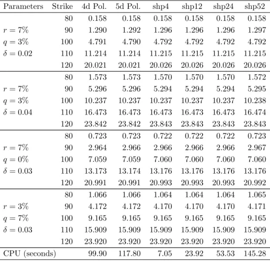
obtained through Matlab (R2010a) running on an Intel Xeon X5680 3.33GHz processor. Table 1 reports American-style put prices with a time to maturity of six months and assuming an elasticity parameter β = 3, while Table 2 values American-style call options with an expiry date of one year, and under a CEV square root process with β = 1.11 The proxy
of the exact American option price (4th column) is computed through the Crank-Nicolson finite-difference scheme with 15, 000 time intervals and 10, 000 space steps. The optimal stopping approach of Nunes (2009) is implemented with conditional minimization through the Matlab “fmincon” algorithm, and using a four and five degree polynomial specification
10The use of the Nunes (2009) valuation methodology will also allow us to compare the SHP results to be
obtained under the JDCEV model proposed in Carr and Linetsky (2006).
11Note that the value of an American-style call option under the CEV model can be obtained also through
for the early exercise boundary (5th and 6th columns, respectively).12 As suggested by
Nunes (2009, page 1246), the parameters defining the exercise policy are first estimated by discretizing both Nunes (2009, Propositions 1 and 5) using N = 24. Then, and based on this
approximation for the optimal exercise boundary, the early exercise premium is computed via Nunes (2009, Proposition 6) using N = 28 time steps. The last four columns of Tables
1 and 2 contain the American-style option prices generated by the SHP method, which is implemented using the Matlab “fsolve” algorithm for solving the recurrence conditions (28) and (29), subject to the restrictions described in Definition 1, and with n ∈ {4, 12, 24, 52}. Accuracy is measured by the mean average absolute percentage error (over the 20 contracts considered) of each valuation approach and with respect to the exact American option price. Efficiency is evaluated by the total CPU time (expressed in seconds) spent to value the whole set of contracts considered.
[Please insert Table 1 about here.]
[Please insert Table 2 about here.]
There are four points that are noteworthy to highlight in these two tables. First, both methods are accurate: the mean average absolute percentage errors (MAPE) in all tested cases are well below the typical bid-ask spread observed in the market. Second, the SHP method with n = 12 gives similar results in terms of accuracy to the Nunes (2009) approach with a four degree polynomial specification for the early exercise boundary, but with less than half of the computational burden. Third, the SHP method with n = 24 gives more accurate results than the Nunes (2009) approach with a five degree polynomial specification for the early exercise boundary, though using a similar CPU time. Fourth, the computational expenses contained in Table 2 are about half of those presented in Table 1 essentially due to the fact that more than half of the American-style options evaluated in Table 2 are equal to their European-style counterparts, and in these cases both methods become faster.
12The early exercise premium (27) is maximized subject to the terminal condition (32), and imposing that
Tables 1 and 2 compile 40 option prices which obviously do not represent a large enough sample to take more robust conclusions, thus giving only a preliminary flavor of the results. Hence, to better assess the speed-accuracy trade-off between the two methods tested we follow the guidelines of Broadie and Detemple (1996) by conducting a careful large sample evaluation of 1,250 randomly generated American-style put option prices.
Table 3 reproduces the pricing errors of the optimal stopping approach of Nunes (2009) with a five and six polynomial specification for the early exercise boundary (2nd and 3rd columns, respectively) and the pricing errors of the SHP approach for four different evenly-spaced time grids (the last four columns), where all the option parameters, with the exception of β and δ, are extracted from the same uniform distributions as in Ju (1998, Table 3). As before, the true American-style put option price is computed through the Crank-Nicolson finite-difference scheme with 15, 000 time intervals and 10, 000 space steps.13 Even though
both methods produce extremely accurate results, the SHP approach offers the best speed-accuracy trade-off for pricing American-style standard options under the CEV model.
[Please insert Table 3 about here.]
4.1.2. JDCEV model
Armed with the closed-form solutions of European-style options and the corresponding hedge ratios, the implementation of the SHP approach for valuing standard American-style options under the JDCEV model (under both recovery assumptions) follows straightforwardly.
To illustrate the robustness and efficiency of the proposed pricing methodology, we focus on the valuation of standard American-style puts under the JDCEV model, though the
13It is well-known—see, for instance, Schroder (1989) or Larguinho et al. (2012)—that option pricing
under the CEV assumption is computationally expensive especially when β is close to two (the lognormal case), volatility is low, or the time to maturity is small. For this reason, we have excluded from the original sample option contracts with an elasticity parameter β ∈ [1.75, 2.25], thus leaving 1,085 contracts to be evaluated. Additional results, not reported here but available upon request, show that it takes almost the
procedure is easily adapted for valuing their counterpart calls. To the best of our knowledge, the optimal stopping approach of Nunes (2009) is the only available methodology, until now, for pricing plain-vanilla American-style options under the JDCEV model—now extended for the payment of the recovery value at the maturity date T —, and hence it will be used as our benchmark.
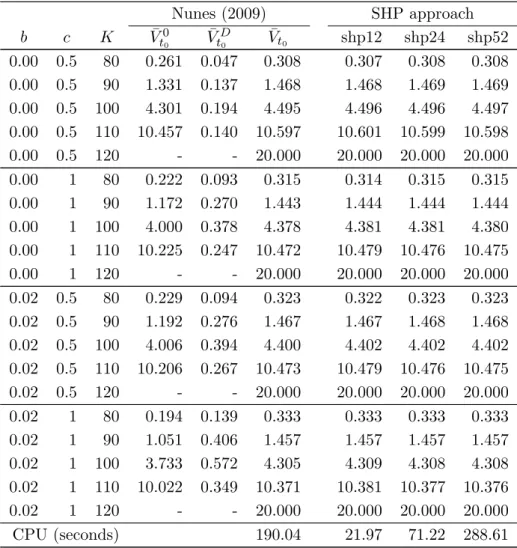
Tables 4 and 5 test the efficiency of the SHP algorithm for valuing standard American-style put options under the time-homogeneous JDCEV model for different parameter confi-gurations borrowed from Carr and Linetsky (2006, Table 1), and assuming, respectively, recovery at maturity (i.e. η = T ) and recovery at default time (i.e. η = ζ). The 4th, 5th, and 6th columns of both tables show the European-style put option price components obtained via equations (13), (9), and (7), respectively. As expected, put options under the fractional recovery of treasury assumption are worth less than the corresponding options under the fractional recovery of face value assumption, due to the different discount effects over the recovery value (equal to K). The optimal stopping approach of Nunes (2009) is implemented with conditional minimization, using the Matlab “fmincon” algorithm, consi-dering a six degree polynomial specification for the early exercise boundary. The parameters defining the exercise policy are first estimated using N = 24 time steps. Then, and based
on this approximation for the optimal exercise boundary, the early exercise premium (7th column of both tables), the American put option price conditional on no default before the expiry and early exercise dates (8th column of both tables), and the present value of the recovery payment made at the maturity date (9th column of Table 4) or at the default time (9th column of Table 5) are computed via equations (27), (24), and (25), respectively, using
N = 28 time steps. The standard American-style put option price contained in the 10th
column of both tables is recovered through equations (23) or (26).14 Finally, columns 11
to 13 of Tables 4 and 5 report the values of the American-style put given in equation (30), which are obtained through the SHP procedure using again the “fsolve” algorithm available in Matlab for solving the recurrence conditions (28) and (29), with n ∈ {12, 24, 52}.
14Both tables highlight that when K = 120 the put is sufficiently in-the-money, so that the time-t 0 spot
price (St0) is already below the critical asset price Et0, and, therefore, the standard American-style put price
[Please insert Table 4 about here.] [Please insert Table 5 about here.]
To sum up, the results computed via the SHP approach are shown to be robust along both tables. For instance, it is possible to obtain extremely accurate option prices (for both recovery assumptions) even using the SHP pricing procedure with only 12 evenly-spaced time points n, but with much less computational burden. As expected, both pricing frame-works require higher CPU times to compute standard American-style put option contracts under the fractional recovery of face value assumption, because, in this case, one has to use a numerical integration scheme for computing equations (19) and (25) under the optimal stopping approach, and equations (19) and (39) under the SHP procedure.15
4.2. American-style capped options
This subsection aims to compare the optimal stopping and the SHP approaches for pricing American-style capped put options under both the CEV and JDCEV models. The valuation of the corresponding calls can be treated similarly.
Table 6 prices American-style capped put options under the CEV model using the para-meter constellations considered in Table 1, but now augmented with a barrier level H = $75. The 3rd and 4th columns of the table highlight the values obtained under the optimal stop-ping approach of Nunes (2009), using equations (26), (27), and (50), with R = (K − H)+,
and considering a polynomial boundary specification with four and five degrees of free-dom, respectively. Columns 5 to 8 report the results obtained via the SHP method with
n ∈ {4, 12, 24, 52}, and computed through the recurrence conditions (52) and (53), and
equation (54). Again, both valuation methodologies have been implemented subject to the restrictions described in Definition 1.
15At the expense of a higher computational burden, both valuation methodologies have been implemented
[Please insert Table 6 about here.]
Table 7 prices American-style capped put options under the JDCEV model (with recovery at maturity) using the parameter constellations considered in Table 4 and a barrier H = $75. The valuation of the corresponding put with recovery at the default time (and calls with both recovery assumptions) can be treated similarly. Columns 4 to 6 value American-style capped put options using the optimal stopping approach of Nunes (2009). The no default component (column 4) is computed using equation (47), and the recovery component (column 5) is computed through equation (48). Finally, column 6 gives the sum of these two components obtained via equation (46).16 The last three columns report the results obtained via the
SHP method with n ∈ {12, 24, 52}, and computed through the recurrence conditions (52) and (53), and equation (54).
[Please insert Table 7 about here.]
In summary, the tables reveal that both pricing methodologies produce results that are almost indistinguishable, though the SHP procedure seems to be more efficient in terms of computational burden. As expected, and as explained in Subsection 3.4, the CPU time required to value these two sets of capped American-style put options contracts under the SHP approach is smaller than the computational effort for valuing the corresponding stan-dard American-style put options of Tables 1 and 4. On the contrary, the optimal stopping approach of Nunes (2009) requires further CPU time, since we still need to find the whole early exercise boundary of the standard American-style put option.
5. Conclusions
The most important theoretical contribution of this paper is the generalization of the SHP procedure for valuing American-style standard and capped options under the JDCEV model
16Similarly to the standard American-style put option case, when K = 120 the capped put is sufficiently
in-the-money, so that the time-t0spot price (St0) is already below the critical asset price Et10, and, therefore,
of Carr and Linetsky (2006). To accomplish this purpose, novel analytical representations were obtained for the hedge ratios of the corresponding European-style standard options, which can be used to jointly price equity and credit derivatives under this general and flexible modeling framework. The SHP approach is also implemented to price American-style standard and capped options under the unrestricted CEV model, thus accommodating both direct and indirect leverage effects typically observed by market practitioners. Furthermore, we extend the optimal stopping approach of Nunes (2009) for the pricing of American-style capped options, assuming that the recovery value associated to the put can be paid at the default time or at the maturity date of the option.
Overall, the numerical experiments run have shown that the SHP pricing methodology is as accurate as but (generally) faster than the optimal stopping approach, thus offering a better speed-accuracy trade-off for pricing American-style standard and capped options under both the (single-factor) CEV and JDCEV models. Nevertheless, and as shown by Nunes (2011, Theorem 1), the optimal stopping approach should be easier to extend for multifactor models (incorporating, for instance, stochastic volatility) because it only requires a numerically tractable solution for both the corresponding European-style option and for the transition density function of the underlying asset process.
Appendix A. Proof of Proposition 1
Nunes (2009, Equations 57 and 60) has already shown that
V0
t0(St0, K, T ; φ) = vt00 (St0, K, T ; φ) + EEPt00 (St0, K, T ; φ) , (A.1)
where the first term on the right-hand side of equation (A.1) is given by equation (8), and
EEP0 t0(St0, K, T ; φ) (A.2) = Z T t0 e−Rt0urldl£(φK − φE u)+− v0u(Eu, K, T ; φ) ¤ SP (St0, t0; u) Q (τe ∈ du| Ft0) .
Assuming that η = T and ζ > t0, equation (25) can be rewritten as VD t0 (St0, R, T ; φ, T ) = (φR)+e− RT t0rldl h 1 − EQ ³ e− RT t0λ(l,S)dl11{τ0>T,τ e≥T } ¯ ¯ ¯ Ft0 ´ −EQ ³ e− Rτe t0 λ(l,S)dl11{τ0>τ e,τe<T } ¯ ¯ ¯ Ft0 ´i , i.e. Vt0D(St0, R, T ; φ, T ) (A.3) = (φR)+e− RT t0rldl h 1 − EQ ³ e− RT t0λ(l,S)dl11{τ0>T } ¯ ¯ ¯ Ft0 ´ +EQ ³ e−Rt0Tλ(l,S)dl11{τ0>T,τ e<T } ¯ ¯ ¯ Ft0 ´ − EQ ³ e−Rt0τeλ(l,S)dl11{τ0>τ e,τe<T } ¯ ¯ ¯ Ft0 ´i , since 11{τe≥T } = 1 − 11{τe<T }.
Equations (10) and (11), and the law of iterative expectations, imply that equation (A.3) can be further simplified into
VD t0 (St0, R, T ; φ, T ) = (φR)+e−Rt0Trldl£1 − E Q ¡ 11{ζ>T } ¯ ¯ Gt0 ¢ +EQ ¡ 11{ζ>T,τe<T } ¯ ¯ Gt0 ¢ − EQ ¡ 11{ζ>τe,τe<T } ¯ ¯ Gt0 ¢¤ = (φR)+e−Rt0Trldl©1 − SP (S t0, t0; T ) − EQ £¡ 11{ζ>τe}− 11{ζ>T } ¢ 11{τe<T } ¯ ¯ Gt0 ¤ª = vD t0(St0, R, T ; φ, T ) − (φR)+e− RT t0rldlE Q ¡ 11{τe<ζ<T }11{τe<T } ¯ ¯ Gt0 ¢ = vD t0(St0, R, T ; φ, T ) − (φR)+e− RT t0rldlE Q £ EQ ¡ 11{τe<ζ<T } ¯ ¯ Gτe ¢ 11{τe<T } ¯ ¯ Gt0 ¤ . (A.4)
Using again definition (11), equation (A.4) can be restated in terms of the restricted filtration F, with respect to which the asset price process S behaves as a pure diffusion process:
VD t0 (St0, R, T ; φ, T ) (A.5) = vD t0(St0, R, T ; φ, T ) −(φR)+e−Rt0TrldlE Q nh 1 − EQ ³ e−RτeTλ(l,S)dl11 {τ0>T } ¯ ¯ ¯ Fτe ´i 11{τe<T } ¯ ¯ ¯ Ft0 o .
Taking advantage of the Markovian nature of the underlying price process S, the outer expectation on the right-hand side of equation (A.5) can be written as a convolution against the density of the first passage time τe, yielding
VD t0 (St0, R, T ; φ, T ) = vD t0 (St0, R, T ; φ, T ) −(φR)+e−Rt0Trldl Z T t0 h 1 − EQ ³ e−RuTλ(l,S)dl11 {τ0>T } ¯ ¯ ¯ Su = Eu ´i Q (τe ∈ du| Ft0) = vDt0 (St0, R, T ; φ, T ) − (φR)+e− RT t0rldl Z T t0 [1 − SP (Eu, u; T )] Q (τe ∈ du| Ft0) = vD t0 (St0, R, T ; φ, T ) − Z T t0 e−Rt0urldlvD u (Eu, R, T ; φ, T ) Q (τe∈ du| Ft0) , (A.6)
where the last two lines follow from equations (11) and (10), respectively.
Combining equations (7), (23), (A.1), (A.2), and (A.6), equations (26) and (27) arise for
η = T . ¥
Appendix B. SHP method in the exercise region
This appendix shows that whenever φSt0 ≤ φEt0 (for φ ∈ {−1, 1}), the standard SHP
pricing equation (31) would overvalue the American-style option. This is explained by the fact that all European-style options (conditional on no default) in the replicating portfolio (with a strike price equal to the value of the exercise boundary) would end in-the-money until the American-style option is exercised, i.e. until the spot price touches the early exercise boundary. On the contrary, when φSt0 > φEt0, all European-style options included in the
replicating portfolio end out-of-the-money until the American-style option is exercised. Next proposition formalizes the aforementioned economic rationale.
Proposition B1 When φSt0 ≤ φEt0, then
Proof. Given that φSt0 ≤ φEt0, let t∗ ≤ T denote the next passage time of the asset price S through the early exercise boundary, i.e. St∗ = Et∗. This date corresponds to the space
time point n − i∗. Replacing t
0 and St0 by t∗ (or n − i∗) and St∗ ≡ En−i∗, respectively, in
equation (31), the value of the SHP portfolio at time t∗ is equal to Vtshpu∗ (Et∗, K, T, R; φ, η) = vt n−i∗(En−i∗, K, T, R; φ, η) (B.2) + n X j=1 wn−j× vt0n−i∗(En−i∗, En−j, tn−j+1; φ) .
Note, however, that all the European-style options with expiry date at times tn−j+1, for j = i∗ + 1, ..., n, that is all the options with a time to maturity equal to (i∗− j + 1) × δt,
have already expired by time t∗, and, therefore, their terminal payoff has been previously
reinvested until time t∗. Hence, v0
tn−i∗ (En−i∗, En−j, tn−j+1; φ) = (φEn−j− φSn−j+1)
+
n−i∗
Y
k=n−j+2
erk×δt, (B.3)
for j = i∗+ 1, ..., n, and equation (B.2) can be rewritten as Vtshpu∗ (Et∗, K, T, R; φ, η) = vt n−i∗ (En−i∗, K, T, R; φ, η) (B.4) + i∗ X j=1 wn−j × vt0n−i∗(En−i∗, En−j, tn−j+1; φ) + n X j=i∗+1 wn−j× (φEn−j− φSn−j+1)+ n−i∗ Y k=n−j+2 erk×δt.
Using equation (28), equation (B.4) can be further rewritten as
Vtshpu∗ (Et∗, K, T, R; φ, η) = φK − φEn−i∗ (B.5)
+ n X j=i∗+1 wn−j× (φEn−j− φSn−j+1)+ n−i∗ Y k=n−j+2 erk×δt.
Finally, and since
φK − φEn−i∗ = Vt∗(Et∗, K, T, R; φ, η)
corresponds to the well known value-matching condition, then equation (B.5) becomes
Vtshpu∗ (Et∗, K, T, R; φ, η) = Vt∗(Et∗, K, T, R; φ, η) (B.6) + n X j=i∗+1 wn−j× (φEn−j− φSn−j+1)+ n−i∗ Y k=n−j+2 erk×δt.
Given that φSt0 ≤ φEt0, we have φSt < φEt for all t < t∗, which makes the last term on
the right-hand side of equation (B.6) almost surely strictly positive. Therefore,
Vtshpu∗ (Et∗, K, T, R; φ, η) > Vt∗(Et∗, K, T, R; φ, η) . (B.7)
Since equation (B.7) holds at any t∗ along the early exercise boundary, equation (B.1) follows
immediately.
If t∗ > T , then all the European-style options in the replicating portfolio would end up
in-the-money, thus augmenting even further the positive difference between the option values
Vt0shpu(St0, K, T, R; φ, η) and Vt0(St0, K, T, R; φ, η). ¥
References
Abramowitz, M., Stegun, I.A., 1972. Handbook of Mathematical Functions. Dover, New York.
Barone-Adesi, G., 2005. The saga of the American put. Journal of Banking and Finance 29, 2909–2918.
Barone-Adesi, G., Whaley, R.E., 1987. Efficient analytic approximation of American option values. Journal of Finance 42, 301–320.
Bekaert, G., Wu, G., 2000. Asymetric volatility and risk in equity markets. Review of Financial Studies 13, 1–42.
B´elanger, A., Shreve, S.E., Wong, D., 2004. A general framework for pricing credit risk. Mathematical Finance 14, 317–350.
Bensoussan, A., 1984. On the theory of option pricing. Acta Applicandae Mathematicae 2, 139–158.
Benton, D., Krishnamoorthy, K., 2003. Computing discrete mixtures of continuous distribu-tions: Noncentral chisquare, noncentral t and the distribution of the square of the sample