Planning Marine Reserve Networks for Both
Feature Representation and Demographic
Persistence Using Connectivity Patterns
Michael Bode1,2*, David H. Williamson2, Rebecca Weeks2, Geoff P. Jones2,3, Glenn R. Almany2,4, Hugo B. Harrison2, Jess K. Hopf2,3, Robert L. Pressey2
1ARC Centre of Excellence for Environmental Decisions, School of Botany, The University of Melbourne, Parkville, Melbourne, VIC, 3010, Australia,2Australian Research Council Centre of Excellence for Coral Reef Studies, James Cook University, Townsville, 4811, QLD, Australia,3College of Marine and
Environmental Sciences, James Cook University, Townsville, 4811, QLD, Australia,4Centre National de la Recherche Scientifique-EPHE-UPVD, Universite de Perpignan, 66860, Perpignan Cedex, France
Abstract
Marine reserve networks must ensure the representation of important conservation features, and also guarantee the persistence of key populations. For many species, designing reserve networks is complicated by the absence or limited availability of spatial and life-history data. This is particularly true for data on larval dispersal, which has only recently become available. However, systematic conservation planning methods currently incorporate demographic processes through unsatisfactory surrogates. There are therefore two key challenges to designing marine reserve networks that achieve feature representation and demographic persistence constraints. First, constructing a method that efficiently incorporates persistence as well as complementary feature representation. Second, incorporating persistence using a mechanistic description of population viability, rather than a proxy such as size or distance. Here we construct a novel systematic conservation planning method that addresses both challenges, and parameterise it to design a hypothetical marine reserve network for fringing coral reefs in the Keppel Islands, Great Barrier Reef, Australia. For this application, we describe how demographic persistence goals can be constructed for an important reef fish species in the region, the bar-cheeked trout (Plectropomus maculatus). We compare reserve networks that are optimally designed for either feature representation or demo-graphic persistence, with a reserve network that achieves both goals simultaneously. As well as being practically applicable, our analyses also provide general insights into marine reserve planning for both representation and demographic persistence. First, persistence constraints for dispersive organisms are likely to be much harder to achieve than representa-tion targets, due to their greater complexity. Second, persistence and representarepresenta-tion con-straints pull the reserve network design process in divergent directions, making it difficult to efficiently achieve both constraints. Although our method can be readily applied to the data-rich Keppel Islands case study, we finally consider the factors that limit the method’s utility in information-poor contexts common in marine conservation.
a11111
OPEN ACCESS
Citation:Bode M, Williamson DH, Weeks R, Jones GP, Almany GR, Harrison HB, et al. (2016) Planning Marine Reserve Networks for Both Feature Representation and Demographic Persistence Using Connectivity Patterns. PLoS ONE 11(5): e0154272. doi:10.1371/journal.pone.0154272
Editor:Chaolun Allen Chen, Biodiversity Research Center, Academia Sinica, TAIWAN
Received:June 17, 2015
Accepted:April 11, 2016
Published:May 11, 2016
Copyright:© 2016 Bode et al. This is an open access article distributed under the terms of the
Creative Commons Attribution License, which permits unrestricted use, distribution, and reproduction in any medium, provided the original author and source are credited.
Data Availability Statement:All relevant data are within the text of the manuscript and its Supporting Information files.
Funding:MB was funded by Australian Research Council (ARC) DECRA DE130100572. MB was funded by ARC Centre of Excellence for
Environmental Decisions. DW, RW, GJ, GA, HH, JH, RP were funded by ARC Centre of Excellence for Coral Reef Studies.
Introduction
The exchange of individuals among patches of spatially-discrete habitat (“connectivity”) has broad implications for how and whether species persist in a region, how they respond to natural and anthropogenic disturbances at both ecological and evolutionary timescales [1,2], and how they should be managed [3–5]. Connectivity contributes to the persistence and dynamics of metapopulations [6,7], and the structure of metacommunities [8–10], through replenishment of local populations and post-disturbance recovery. Connectivity is especially important in the marine environment, where almost all fish and invertebrate species have an obligate and extended pelagic larval phase [11,12], and strong ocean currents can carry dispersing larvae long distances [13–15]. Because of its central role in the life-cycle of reef fishes, connectivity should be considered when designing networks of marine reserves [16–20]. Marine reserves, particularly no-take areas, only constitute a relatively small proportion of important habitats [21], even in the best protected habitats such as the Great Barrier Reef Marine Park in Australia [21]. Because reef fish populations outside marine reserves are generally depleted [22], and in some contexts (e.g., the Philippines) almost non-existent [23], connectivity is required for these separated protected areas to exchange enough larvae to support persistent populations, and also to provide the spillover that exports their benefits to the broader, unprotected landscape [24].
Marine reserve networks must therefore satisfy two constraints simultaneously. First, they should guarantee the representation of key conservation features in the reserve network. This is a primary goal of all systematic conservation planning [25]. Important facets of biodiversity such as species, habitat types, and ecological processes should occur within no-take reserves, somewhere in the network (a“feature representation constraint”). Second, the networks should ensure that sufficient larvae are being exchanged between populations to ensure that those pop-ulations will persist into the future (a“demographic persistence constraint”) [18,26]. This requires connectivity to be incorporated explicitly. While understanding the process of larval connectivity is critical to the success of marine reserve networks [4,27], most systematic conser-vation planning theory has focused only on feature representation, with a range of planning tools available to implement these theories [25,28]. However, these tools do not currently include persistence constraints; as a result, while the tools represent conservation features, it is unknown whether those features will be able to persist. In fact, there is reason to believe that reserve networks which only target representation constraints will fail to achieve persistence constraints. Potential reserve sites that are further apart are likely to exhibit greater differences in species composition, and therefore to be selected in an efficient complementary reserve sys-tem. However, such sites are less likely to be demographically connected (and are therefore less likely to persist) because dispersal strength diminishes rapidly with distance [26,29,30].
Planning for marine connectivity has historically been constrained by a lack of modelled or empirical data. In-situ observations of larval dispersal are almost impossible, because the density of dispersing larvae in the planktonic environment is vanishingly small [5,31]. Nevertheless, in the last decade, quantitative larval dispersal data have become available for an increasing num-ber of species and locations, at ever greater spatial scales and higher resolutions. Some of this information has come from population genetics [32,33] and biophysical modelling [13,34,35], which have estimated larval connectivity over very broad spatial and temporal extents [17,36–
39]. Simultaneously, the recent emergence of methods for genetic parentage [24,40,41] and oto-lith microchemistry [40,42] have begun to provide empirical dispersal data across spatial and temporal scales that are relevant to spatial management planning. Unfortunately, this new dis-persal data has revealed fundamental limitations to conservation planning theory.
cannot be guaranteed. However, most conservation planning methods cannot incorporate dynamical processes such as connectivity. Systematic conservation planning theory calculates the performance of potential protected area locations via data on features and processes [25,43]. To date, these methods have almost exclusively used static data on biodiversity, such as the location of habitat types, or static species distribution models [44–46]. Acknowledging the importance of dynamical processes, researchers have made a series of modifications to their standard methods for planning that allow them to include connectivity. These modifica-tions fall into four categories; for a variety of reasons, each is unsatisfactory. The most common category applies quantitative“rules of thumb”for MPA size and spacing [47,48]. While straightforward and often derived from empirical data on connectivity, these rules involve overly simplistic assumptions that ignore spatial heterogeneity in habitat availability and dis-persal patterns. The second approach uses connectivity patterns to rank habitat patches, gener-ally using metrics from network theory (e.g., centrality, or eigenvalue analysis; [49–53]). While these metrics make some intuitive sense, they have no clear ecological or demographic inter-pretation [54]. It is therefore unclear if the resulting reserve networks ensure persistence. The third approach ranks planning units using connectivity directly, but focuses on only a small subset of the data, such as the self-recruiting proportion [52,53], even though metapopulation persistence depends on dispersal between populations [13,55]. The fourth approach is to treat connectivity as a feature that requires representation in the reserve system, similar to species occurrences [56–58], including widely used methods such as Marxan’s boundary-length modi-fier [59]. Doing so makes the unreasonable assumptions that connectivity can be traded-off within and between species, and that lower connectivity can be tolerated if the reserve network is cheaper or larger. Such approaches also treat connectivity as a fundamental conservation objective, rather than a means of ensuring that species persist. Because none of these four approaches incorporate connectivity into an explicit demographic process, the performance of the resulting reserve networks (and thereby the underlying approaches) must be assessedpost hocusing population viability analyses that explicitly evaluate persistence [50,52,53]. Such assessments are not common however, and even if their results provide indirect validation of an approach, a more direct inclusion of connectivity into the life-cycle of the species of interest is still preferable.Post hocvalidation also cannot explain what aspect(s) of indirect approaches to connectivity planning were successful or not in achieving persistence.
A wide range of tools and methods are available to ensuring reserve networks are representa-tive [28]. However, there are two main challenges to correctly incorporating connectivity along-side representation. First, from an ecological perspective, managers need to be able to translate the new data on larval dispersal into quantitative expressions of how much dispersal is needed to guarantee demographic persistence in each planning unit. For coral reef fishes, these require-ments will need to be based on the full complexity of the larval connectivity patterns (i.e., not just self-recruitment), but also critical post-recruitment demographic processes such as mortal-ity and reproduction—connectivity patterns aren’t enough by themselves. Second, from the per-spective of conservation planning, methods are needed that include constraints for
demographic persistence, and then integrate them with the representation constraints of multi-feature conservation planning. To address these challenges, we describe a new analytical method for designing MPA networks that satisfy the dual constraints of feature representation and—via connectivity patterns—the persistence of species with obligate larval dispersal phases.
Methods
represented, and also a set of target species whose persistence needs to be guaranteed. These features and species are distributed among a set of planning units. We then demonstrate the application of this method by parameterizing it for a study area—the Keppel Islands group within the Great Barrier Reef Marine Park, Australia. This case study shows how the general model is parameterized, in particular how recruitment constraints can be defined.
Management constraints and the objective function
In a seascape (i.e., a marine landscape) ofPplanning units (reefs, sections of coastline, etc), marine reserve networks are defined by the binary vectorN, whose elementsNiindicate whether planning unitiis protected (Ni= 1) or unprotected (Ni= 0). Managers need to choose a reserve network that will equal or exceed two separate sets of constraints, while maximising an objective function. The first constraint ensures that a sufficient amount of each important conservation feature is found within the reserve network (the feature representation con-straint). The second constraint ensures that every target species, in each protected or unpro-tected patch, receives enough recruitment to replenish populations and maintain persistence at a metapopulation scale (the demographic persistence constraint). Our method satisfies these two constraints while minimising a network performance metric: the reduction in fishing opportunities resulting from the no-take reserves.
Constraint 1: Represent conservation features within the marine reserve network. Each planning unit contains a known amount of each feature of conservation interest (total ofF fea-tures, e.g., habitat, ecological processes or species), stored in a (P×F) matrix denotedM. Man-agers define constraintsQkthat correspond to each conservation featurek. An adequate reserve network will protect a set of planning units such that the total amount of each feature protected equals or exceeds its respective representation constraint.
X
Pi¼1
Ni ½Mi;kQk; 8k: ð1Þ
Constraint 2: Ensure the demographic persistence of key species. Each planning unit hosts populations ofSnon-interacting species that experience fishing mortality, either as target species or bycatch, and whose dynamics can be described using metapopulation models. The species all have sessile life-history strategies, that is, adults do not move between distinct reef patches, but populations are demographically connected via the dispersal of larvae. For each speciess, the amount of dispersal between each planning unit is defined by twoP×P recruit-ment matrices,R
sandRs. The element on rowiand columnjin each recruitment matrix rep-resents a number of dispersing juveniles produced in planning unitithat would survive dispersal to settle and recruit in planning unitj. Thefirst matrix,½R
sij, states the recruitment that will occur when the source patch,i, is unprotected, the second, [Rs]ij, states the additional recruitment (i.e., above the level offered by an unprotected source) that would occur if that source population were protected. For the case study that follows, we define the recruitment matrices using dispersal kernels, but note that they can be defined by any description of con-nectivity, and that they can be asymmetric, contain large-scale structure, or not be strongly connected [15,60–63].
achieve this constraint, then populations in protected planning units will persist, since well-enforced no-take reserves will only experience natural mortality. On unprotected planning units, this level of recruitment will not be sufficient to maintain fished populations at the same densities as in reserves. However, it will be sufficient to maintain persistent sink populations in unprotected planning units, and therefore to support ongoing catches. Calculating this con-straintTi,sis therefore equivalent to calculating natural mortality rates and the recruitment needed to replace it. We illustrate how this is done for the Keppels case study below.
The demographic persistence constraint is expressed as:
XP
i¼1
ðNi½Rsijþ ½R
sijÞ Tj;s; 8j8s: ð2Þ
The second term in the summation (the recruitment from unprotected planning units) does not depend on the control valuesNiand is a constant. It could therefore be moved to the right hand side of the inequality. This would change the constraint from a minimum total recruit-ment, into a minimum additional recruitment coming from inside the reserve network. We also note that we can incorporate the common“scorched-earth”assumption (where popula-tions on unprotected planning units are equal to zero) into our model by addingR
stoRs, and replacingR
s with zeros. Finally, while this formulation assumes that connectivity is constant through time, the basic form ofEq (2)can be modified to incorporate temporal variation in lar-val dispersal patterns [13]. If connectivity matrices from different years are incorporated into the constraint as pseudo-species, the resultant reserve network would satisfy the demographic persistence constraints for every year in the dataset.
The demographic persistence constraints will generally vary with the identity of the plan-ning uniti. These factors can therefore reflect spatial heterogeneity in the habitat quality of planning units, such as different rates of mortality, different population densities, or different reproductive rates. In terrestrial population viability analyses, such factors are often derived from correlative ecological niche models [64], or spatial ecophysiological models [65], although this is not as common for marine species. The elements of the recruitment matrices are also able to vary, depending on both the output of the source reefs, and the potentially heteroge-neous larval dispersal patterns between the planning units. Unprotected reefs will produce fewer recruits in our analyses since they support fewer reproducing adults, but output can also vary with the quality of the source habitat, or the direction and strength of ocean currents [15]. The formulation ofEq (2)ignores transient dynamics and therefore the constraints will only be guaranteed once the reserve network has been in place for time periods that are longer than the generation times of the focal species, and assuming that the system has not passed any irrevers-ible abundance constraints.
Objective function: Minimize forgone fishing. We assume that the protection of any planning unit (Ni= 1) will have a negative impact on local extractive activities that can be decomposed into two multiplicative factors. These are the abundance of each species found in each planning unit when it is fished,bi,s, and the value of an individual of speciessto the fish-ers, relative to the most valuable species,Vs. Management wants to satisfy the conservation constraints while minimizing the sum of this impact across the network. Therefore, the manag-ers’objective is to minimize:
min
N
X
Pi¼1
NiWi; ð3Þ
whereWi¼S S
account the potential responses offishers to the closure offishing grounds [66,67]. The likely impact of implementing reserves is an increase in the intensity offishing effort on unprotected planning units, the so-called“squeeze effect”of displaced effort. If thefishery was not
over-fished before reserves were established, this displaced effort on unprotected reefs can result in lower spawning stock biomass, reduced harvests, and higher per-unit extraction costs. This would make the absolute value of our objective function an underestimate offishery impacts, although it may not alter the relative performance of different reserve networks.
Finding the optimal solution
Each of the elements in this problem—the performance metric and both constraints—are lin-ear, and the optimal solution to this problem can therefore be found by applying binary integer programming methods [28]. We describe in detail how the above problem can be thus formu-lated inS1 Text.
Case study: Keppel Island group, Great Barrier Reef Marine Park
The Keppel Islands group is an archipelago of high continental islands off the central Queens-land coast, within the Great Barrier Reef Marine Park (GBRMP) (Fig 1). The fringing coral reefs support large populations of bar-cheek coral trout (Plectropomus maculatus), which is one of the key target species of the reef line fishery operating in the GBRMP [68]. The species is also a favourite species of local recreational fishers, and has been the focus of recent intensive research on its life history and dispersal abilities [24,69,70]. Approximately 700 ha of fringing coral reefs within the island group are protected by a multiple-use zoning management plan that includes areas that are open to fishing (recreational and commercial), and a network of limited-use and no-take reserve areas [21]. Since the rezoning of the GBRMP in July 2004, approximately 28% (196 ha) of the reef area within the Keppel Island group has been protected within no-take reserves. To demonstrate a hypothetical application of our general method, we devised ade novoreserve network for this island group, concentrating on protecting three habi-tat features and ensuring the persistence ofP.maculatus.
Feature representation constraints. We began by defining 36 planning units across the region (Fig 1b–1d). Some planning units contain a single patch reef, some contain a part of a larger reef or island, and some contain multiple small patch reefs. These 36 planning units align with the current zoning plan for the Keppels region, which includes three coral reef man-agement zones: Habitat Protection Zones (HPZ); Conservation Park Zones (CPZ); and Marine National Park (no-take) Zones (MNPZ) [71]. Due to the close proximity to the mainland and ease of access, fringing reefs in the Keppel Islands are almost exclusively fished by recreational fishers, for whom HPZ and CPZ reefs are open to fishing (Williamson et al. 2014). Our plan-ning method consequently considers these two zones to be unprotected (Ni= 0), and MPNZs to be protected (Ni= 1).
Keppel group and the GBR as a whole. Data on the distribution of habitat types were calculated using ground-truthed satellite imagery in ArcGIS. The resulting feature matrixMis inS1 Table.
Demographic persistence constraints. The following section details how we choose con-straints for annual recruitment into each planning unit (Ti,s) which ensure that all protected Fig 1. (a) Location of the Keppel Islands on the east coast of Australia. Individual reefs in the Great Barrier Reef are shown with light blue markers. The red box indicates the specific location of the Keppel Islands in the southern GBRMP. The remaining figures show the detailed location of the Keppel Islands and different optimal reserve networks. Colored polygons indicate the planning units: no-take reserve in green, non-reserve in blue. (b) The reserve network that satisfies constraints for both feature representation and demographic persistence, while minimizing the opportunity costs to fishers. (c) The reserve network that satisfies the feature
representation constraints at a minimum cost to fishers. (d) The reserve network that satisfies the demographic persistence constraints at a minimum cost to fishers. The map incorporates data which is the copyright of the Commonwealth of Australia (Great Barrier Reef Marine Park Authority), and used with permission of the Commonwealth. The Commonwealth has not evaluated to Data as altered and incorporated, and therefore gives no warranty regarding its accuracy, completeness, currency or suitability for any particular purpose.
planning units receive sufficient recruitment to exceed or equal natural mortality rates. Unpro-tected reefs receive at least the same level of recruitment, which will sustain ongoing catches (though not pristine densities). Self-recruitment will be a key component of this recruitment, and is included in our models. However, the estimated scale of larval dispersal [29], and observed dispersal between marine reserves [24], strongly suggest that adequate recruitment will require immigration from other reefs. Our method takes both sources of recruitment into account, using the recruitment matrices to measure their relative contribution.
Based on a von Bertalanffy growth curve parameterized forP.leopardus(a closely-related sister-species; [75]), we estimate thatP.maculatusindividuals in the first-year class (from recruitment to age one) have a fork length of25 cm. Surveys of the abundance and size of the species on the slope habitat of existing protected reefs report an average of 46 such individ-uals per hectare. These 46 individindivid-uals are the survivors of larger settling cohorts, and to convert this density into a recruitment target for each planning unit, we correct for two different forms of mortality. First, recruits experience a very high rate of mortality in the first 48 hours post-settlement, estimated at 56% [76]. Following this, a study estimated the average ongoing mor-tality rate ofPlectropomusspp. recruits in their first year at 60% [77], which is equivalent to a daily mortality rate of 0.25%. Assuming that larvae arrive at a constant rate throughout the year, these mortality rates imply that the 46 surviving individuals per hectare in the first year age class are the result of 160 settlers/hectare of slope habitat annually.
We adapt this constraint to create values forTi,sin each planning unit. The density of repro-ductively mature female adults in each habitat type, in protected reefs, was estimated using habitat stratified counts carried out throughout the Keppel Islands in 2008, which estimated the density and length-frequency distributions of all adultP.maculatusindividuals. On the reef crest, slope and flat, adult densities are 48, 99 and 26 individuals per hectare, respectively. Since each habitat type exhibits similar size structures, we use these relative densities to calcu-late recruitment constraints of 78, 160 and 42 settlers per hectare of crest, slope and flat. As an example of how the differentTi,svalues are calculated from these densities, the planning unit that surrounds Barren Island contains 13, 26.2, and 1.9 hectares of reef crest, slope and flat respectively (seeS1 Table). We therefore want to create a reserve network that will deliver a total of 5,277 larvae to the Barren Island planning unit.
Recruitment data (Rs). Empirical data and biophysical modelling have demonstrated sig-nificant levels of larval retention and exchange forP.maculatuswithin and among reefs in the Keppel Island group [24]. The destination of larvae that are spawned within each planning unit is determined by a combination of oceanographic influences and larval behavior. Oceanography is driven by a strong local tidal regime, the broader Mackay macro-tidal regime, seasonal wind-driven connectivity with the larger Capricornia group of reefs, and episodic events of the south-ward-flowing East Australia Current.P.maculatuslarvae have relatively long pelagic larval dura-tions of 24–29 days [24]. Larvae are thought to be released in small-group spawning aggregations that occur between October and March inclusive [78], for five days either side of new moons.
We estimated this dispersal using recruitment matricesRsandRs, based on data gathered forP.maculatusin the Keppels region, where a large parentage assignment experiment sam-pled juveniles and adults from across the Keppels between 2007–2009 (Harrisonet al. 2012). Parentage samples could not be used directly to create recruitment matrices because only a subset of reefs were sampled, and because parentage could only be assigned to a subset of sam-pled recruits. To extrapolate this data across all planning units, we thereforefit larval dispersal kernels to the data [79]:
pij¼ 1
2p2exp dij
Where the Euclidean distance between reefs is denoteddij, and is used to predict the probability pijthat a larvae spawned at planning unitiwould disperse and settle on planning unitj, conditional on it surviving the larval phase. The parameterϕis estimated at 12.38 for the Keppels. We trans-form these proportions into the number of settlers by multiplyingpijby the total number of larvae produced annually in each planning uniti. The number of larvae that travel from unprotected planning unitiand recruit to any planning unitj(i.e., protected or unprotected) is therefore:
½R
sij¼ypij
X
3h¼1
X
15
y¼1
fyai;hyr
y;s;h ð5Þ
wherefyis the fecundity of a female of length classy. Each length class is 5 centimetres, with the maximum length observed equal to 75 centimetres; the length of each class is estimated using the upper bound of the class, designatedly.ϕyis the proportion of adults in length classywho are female, andθis the proportion of spawned larvae who die during the dispersal phase. The vari-ablesr
y;s;hrepresent the density of adults of speciessand lengthyin habitathon unprotected reefs (ρy,s,hgives the density on protected reefs), andαi,his the amount of habitat of typehin plan-ning uniti(his either 1: crest, 2: slope, or 3:flat). We can calculate [Rs]ijby substituting
(ry;s;h r
y;s;h) forr
y;s;hinEq (5). For the remainder of this section, we go through our process of estimating each of these parameters. Note that, while our probabilities of dispersal are symmetrical (i.e.,pij=pji), the recruitment matrices are not, since the source populations are different (S1 Fig).
In the Keppel Islands, all reef habitats are defined as reef crest, slope or flat (the areaαi,h, of each is the same as in the feature matrix). Each of these habitat types supports a different adult density, but approximately the same age-distribution (Kolmogorov-Smirnov test,α= 0.01). The density of reproductively mature adults of a given lengthρy,son protected reefs is estimated using habitat stratified counts as described in the recruitment section above. Their relative densities in protected and unprotected planning units were estimated in 2009, when a set of surveys was undertaken at 22 monitoring sites, on both reserve (MNPZ) and non-reserve (HPZ, CPZ) reefs. The results indicate that mean adult coral trout density is 1.8 times higher on reserve reefs than on non-reserve reefs. We assume that this proportional difference in densities between reserve and non-reserve reefs is consistent between the three habitat types, which themselves have differ-ent densities (already described). As a consequence of the differdiffer-ent habitat distributions in each planning unit, the elements of the recruitment matrix vary greatly, reflecting both the habitat quality in the different planning units, their protected status, and the distance to the nearest larval destinations. Large reefs with higher proportions of slope habitat, that are both protected and close to other planning units, have the potential to operate as demographic sources in the meta-population, and will therefore be prioritised for protection by the optimisation algorithm.
A changing proportionϕyof adults are female, since the species is a protogynous hermaph-rodite. The sex ratio of the individuals in different length classes was inferred from previous studies of the size-sex structure ofP.leopardus, another protogynous hermaphrodite [80]. This study showed thatP.leopardusin the central GBR begin to transition from female to male at a length of 32cm, and are exclusively male at lengths above 52cm. We therefore model the female proportion of the population as a linear relationship with length:
y¼
1 if y<7
x 7 4 if
7y11
0 ify>11 8
> > > <
> > > :
ForP.maculatuswe estimate the fecundityfyusing published allometric relationships for species in the genusPlectropomusthat link length and fecundity [81]:
fy¼13:82ðlyÞ
3:03
: ð7Þ
The larval mortality proportionθis a very difficult component to parameterize. Larval mor-tality is thought to occur chiefly through predation, and literature estimates of the rate vary between 2% and 97% per day [82]. Given this uncertainty, we choose a value forθthat can rec-reate the adult abundance currently observed in the Keppels, consistent with our model of the metapopulation. Using the surveyed estimates of adult density (ρandρ), the location of the
current marine reserves in the Keppels, and estimates of larval dispersal derived from the best-fit kernels (pij), we vary the value ofθuntil all of the current MNPZ zones received sufficient recruitment to justify their current populations (as described above, 78, 160 and 42 settlers per hectare of crest, slope and flat). These values imply that a mortality parameter ofθ= 7× 10⁻⁴
will recreate the observed recruitment densities, a daily mortality rate of 26%. SeeS1,S2andS3 Tables for recruitment data used.
Objective function. The recreational fishing community is the largest and arguably the most politically powerful stakeholder in the GBRMP, and were an influential voice during the 2004 rezoning of the GBRMP [83,84]. They are particularly important in the Keppel Islands, where the vast majority of the fishing effort applied to the reefs is from the recreation sector. The consumptive interest of recreational fishers in the GBRMP is focused on the number and size of fish caught during trips, with a premium placed on catching the mandated daily limits (bag limits) of large fish, and an additional aversion to trips that catch nothing [85]. Once the constraints for representation and persistence are satisfied, we assume that the primary con-cern of managers is to minimize the aggregate opportunity cost of the no-take reserves on rec-reational fishers. Specifically, to minimize the total number of fish that are no longer accessible to fishers because of the location of the no-take reserves.
We only consider one fish species, so we setV1= 1 without loss of generality. We base the value of each planning unit on the number of adult individuals longer than the length restric-tion that exist on that planning unit when it was fished (38 cm total length) [86]. The total number of legal sizedP.maculatusin each planning unit is estimated using the same 2009 hab-itat-stratified count data described above. The objective function therefore takes into account the relative suitability of the different habitat types. An alternative objective function based on lost access to coral trout biomass would also be straightforward to implement using these sur-veys and published allometric relationships between length and weight [17].
created using the three different approaches, to the amount of overlap observed within a set of 10,000 reserve networks, each made up of a comparable number of randomly selected planning units.
We further assess the degree to which persistence constraints were complementary to repre-sentation constraints. To do this, we calculate how the amount of area protected by a feature representation network needs to increase if managers want to satisfy the demographic con-straints without explicitly planning for them. If planning units contributing highly to both representation and recruitment overlap, then recruitment constraints may require only small additions to the marine reserve network (or no additions at all). However, if planning units important for representation and recruitment are not congruent, the required increase in the coverage of no-take reserves could be substantial.
Sensitivity analyses. As we emphasise during our parameterisation of the Keppels case study above, many of the ecological parameters in these analyses are challenging to estimate. This is particularly true for the larval dispersal parameters (e.g., the daily rate of pelagic larval mortality), which are difficult to observe directly. Moreover, the feature representation and demographic persistence constraints are also difficult to define with confidence, particularly since they involve a combination of difficult empirical questions (e.g., what is the relative spawning stock biomass on reserved and fished reefs?) and complicated value-judgements (e.g., what level of coral reef degradation is the community willing to tolerate?). We conse-quently undertake a sensitivity analysis for our Keppels case study, focusing on the effects of uncertainty in both the ecological parameters, and the size of the constraints.
We vary four uncertain elements of the formulation—two different parameters, and the two constraints. In each test, we assess how robust the optimal reserve design is to pessimistic uncertainty. Instead of assessing whether the reserve design changes with a single arbitrary amount of uncertainty (e.g., withinx= 5%), we calculate how much uncertainty the optimal network can tolerate before it fails to achieve both its demographic and feature representation constraints. The tests are: (1) we randomly increase each of the feature constraint levels (Qk) within ±x% of their original values. This corresponds to uncertainty about how much of a given feature needs protection to ensure it can persist into the future. (2) We alter each demo-graphic recruitment constraints (Ti,s) within ±x% of its original value, to reflect our uncertainty about how much recruitment is needed to maintain persistent populations on protected reefs. This is a particularly important sensitivity test to undertake, given the challenge of estimating these constraints. (3) We decrease the amount of each habitat type in each planning unit by withinx% of its nominal value. The distribution of habitat across planning units is based on ground-truthed satellite data, but will still contain error at the high resolution of these analyses. (4) Finally, we decrease each element in the two recruitment matrices (RsandRs) by withinx %. Thisfinal sensitivity test, which varies values in the recruitment matrices, can represent uncertainty in a wide range of ecological parameters, including larval mortality or pre-capita fecundity (seeEq 5). We only consider pessimistic uncertainty in thefinal two sensitivity analy-ses, since we are calculating how incorrect we can be in our parameter estimates while still meeting the constraints. Varying the parameters by increasing them will obviously continue to satisfy the constraints.
Results
36% of reef flat, crest and slope habitats respectively (Fig 1b). The network therefore exceeds the nominal constraints for feature representation (35% of each habitat), particularly for reef slope. In keeping with the spatially heterogeneous nature of larval dispersal, the optimal reserve network delivers widely different amounts of recruitment to the different planning units: one receives only 102% of its constraint, while another receives 110 times its constraint. Given that coral reef fish larval recruitment is believed to be space-limited [88], both of these planning units would contain comparable densities of adults, with the latter experiencing higher levels of compensatory mortality. The dual constraint reserve network satisfies these constraints by excluding fishers from planning units that contained 40% of the fishable biomass in the system.
The feature representation network (Fig 1c) is the same size as the dual constraint network, and protects almost exactly the constraint amount of the three reef habitat types (37%, 36% and 35% of reef flat, crest and slope habitat respectively), and therefore 36% of the total reef area in the Keppel Islands. Because it does not seek to achieve the recruitment constraints, two planning units in the system do not receive adequate levels of recruitment (they received 85% and 95% of the constraint). While this is not a large deficit, and while these planning units rep-resent a small subset of the reserve network, this shortfall means that persistence cannot be guaranteed within all planning units. Reserved planning units experiencing a shortfall would no longer necessarily export as much larvae as expected, and this would compromise the per-sistence of all downstream reefs. The feature representation reserve network incurs a lower opportunity cost on fishers, excluding them from planning units that contain 36% of the fish-able biomass in the system. The network designed to achieve only the recruitment constraints (Fig 1d) is different again. This network is much larger than the others—protecting 17 planning units—and provides very different habitat representation: 2%, 46% and 41% of reef flat, crest and slope habitats respectively, and 27% of the total reef habitat area. The network imposes an opportunity cost on recreational fishers that is approximately equivalent to the other networks.
We use the proportional overlap between the different reserve networks to assess whether satisfying the different constraints (representation-only, persistence-only, dual-constraint) requires different sets of planning units. The planning units chosen by the three optimal reserve networks are visibly different (Fig 1), but there is still some overlap. The persistence-only and representation-only reserve networks have an 11% overlap, as do the persistence-only and dual-constraint networks. However, this does not indicate that the planning units selected by multiple networks are particularly important, nor that the networks are significantly similar, since this amount of overlap is seen in random networks of the same size. Similarly, although the dual-constraint and representation-only networks have much less overlap (sharing only 3% of their planning units), given the smaller size of their networks, even this small amount of overlap is not significantly more or less than random expectation.
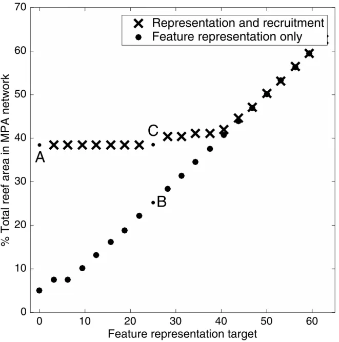
(shown spatially inFig 1d). The marker indicated by‘B’represents the reserve network designed only for habitat representation (shown spatially inFig 1c). The marker indicated by
‘C’represents the dual constraint network.
Optimal reserve networks—particularly those based on constraints—are notoriously sensi-tive to parameter uncertainty, since the design algorithms aim to meet the constraints as exactly as possible, in order to minimise the objectives, which are normally acting in opposition (e.g., minimise costs). We therefore explore the tolerance of our optimal network to pessimistic Fig 2. Relative strength of the two constraints on the conservation plan.The constraint for feature representation increases along the x-axis. Black crosses show the size of the no-take reserve networks required to optimally satisfy both constraints, with the demographic persistence constraints kept constant at our calculated values and the feature representation constraint increasing from left to right. Grey circles show the protection needed to optimally meet the constraints for feature representation, but not the constraint for demographic persistence. The marker‘A’is equivalent to the reserve network inFig 1d. The marker‘B’is equivalent toFig 1c. The marker‘C’is equivalent toFig 1b.
uncertainty in both the demographic parameters, and in the two different constraints. In gen-eral, the optimal reserve network is far more tolerant to pessimistic variation in the demo-graphic persistence constraints and recruitment matrices, than it is to pessimistic variation in the feature representation and the distribution of habitat types. The optimal network is able to satisfy both sets of constraints while: (1) the increase in the feature targets remains within 1%; (2) the increase in the demographic persistence targets remains within 50%; (3) the decrease in the amount of habitat features in each planning unit remains within 1%; and (4) the decrease in the elements of the recruitment matrix remains within 21%. If the amount of variation is less than these amounts, the reserve network can still achieve both sets of conservation constraints for 95% of randomly altered systems.
From these results, it is clear that the optimal reserve design is far more sensitive to variation in the habitat features and targets. This outcome can seem counter-intuitive, since feature representation targets are far easier to achieve in the Keppels Islands case study than demo-graphic persistence targets (Fig 2). However, feature representation has fewer dimensions than recruitment (i.e., there are only three habitat features, and hundreds of elements in the recruit-ment matrices), and features are more evenly distributed among the planning units than recruitment. As a result, the algorithm is generally able to find a reserve network that efficiently achieves the feature representation targets, with a negligible amount of surplus feature protec-tion. While this makes the optimal reserve network efficient from a feature representation per-spective, it means that changes to the network can easily compromise those targets. In contrast, demographic persistence targets are harder to meet perfectly, and therefore are often over-achieved. The networks are consequently more robust to uncertainty about dispersal.
The solution approach, implemented in Matlab’s binary programming function (bintprog; Matlab 2012), applies a linear-programming based branch-and-bound algorithm. On a desktop computer, this method identified the optimal solution for the Keppel Islands problem (36 plan-ning units) in under a second. The runplan-ning time of binary programming methods increases nonlinearly with problem complexity (the number of planning units in this case). Based on an analysis of systems with randomly generated features and dispersal patterns, applying our method to a problem with 50 planning units takes less than half a minute, while 100 planning units would take approximately 2 hours.
Discussion
Here we advance a methodological approach that provides an explicit and mechanistic approach to adding demographic persistence constraints to standard feature representation systematic conservation planning approaches. The methods are specifically tailored for patchy marine ecosystems with demographically essential larval connectivity. Furthermore, our case study demonstrates that the required constraints for demographic persistence can be parame-terized, albeit in a data-rich coral reef ecosystem. While systematic conservation planning strives to represent the full extent of biodiversity and also to ensure long-term persistence within managed areas [25], to date it has been more successful at the former goal than the lat-ter. Our successful inclusion of population persistence into a systematic conservation planning framework addresses this issue and we illustrate how it can be applied in a data-rich context.
the introduction, are not explicitly linked to the persistence requirements of particular species [4,48]. It is therefore unclear if they would achieve their stated purpose without the application of separate,post hoctesting [89]. The second set of approaches are very explicit in their incor-poration of ecological processes, including connectivity. Researchers are now creating deci-sion-support tools that extend population viability analyses (PVAs) to incorporate spatial processes and conservation actions such as protected areas. These methods approach the prob-lem of reserve design from the direction of population ecology, in contrast to the biogeographic origins of systematic conservation planning. The tools generally couple ecological niche model-ling with stochastic population simulations [90–94], and are primarily applied to terrestrial conservation problems. Because they describe processes like connectivity explicitly and mecha-nistically, they are naturally suited to including connectivity information. However, while such approaches are mechanistic, consider uncertainty explicitly, and can be meaningfully parame-terized [64,94], they are too computationally intensive to apply to the millions of possible reserve networks that need to be assessed in the process of systematic reserve network design. The methods are therefore best suited to assessing the relative performance of a small number of potential configurations in well-studied ecosystems (i.e., management strategy evaluation; Bunnefeld et al. 2011).
Our method occupies the space between these two approaches. It attempts to retain much of the practical simplicity that is the strength of the qualitative design criteria by expressing persistence (a dynamic process) as a set of static constraints (Eq 2). This approach allows per-sistence to be incorporated into the same well-tested optimization techniques as feature repre-sentation. However, like the spatial PVA approaches, our method is also based on a
mechanistic description of population processes, and the constraints that it sets are explicitly linked to the overall conservation goals of demographic persistence. It is therefore able to make explicit and testable predictions about persistence, and to use ecological data to inform the con-cept of“adequate protection”. Because it offers an intermediate level of complexity and process, our method cannot displace either of the two existing alternatives. Qualitative design criteria (e.g., size and spacing rules) will still be required when decisions are needed with little informa-tion, a situation that applies across the tropical world, and for many critical coral reef fishery species even in developed economies. At the other extreme, spatially- and temporally-explicit PVAs will provide more accurate guidance when data and computational time are not limiting, and when only a small number of alternative scenarios need to be assessed. However, many sit-uations exist between these two extremes, and methods such as ours therefore have the poten-tial to provide useful and rapid decision-support in appropriate situations. Computationally, our method ran for the Keppels case study in under a minute. Although larger problems will take longer, heuristic methods such as simulated annealing (Kirkpatrick et al. 1983) or tabu search (Glover 1986) can help speed up the process.
over representation constraints may not be true for every case study. Nevertheless, whenever conservation planning undertakes multi-constraint planning, one set of constraints is likely to be much harder to satisfy than the others. The conservation planning problem then simplifies to a problem addressing a single set of constraints—demographic persistence in the Keppel Islands case study—with the other set(s) being satisfied incidentally, in the process of satisfying the binding constraints (e.g.Fig 2). Once the binding constraints have been identified, the resulting simplified problem can potentially be solved with much less information, and with greater atten-tion to the specifics of the more important process or pattern.
The second insight is that in dispersive environments such as marine ecosystems, the funda-mental goals of conservation planning—that of representing a heterogeneous and multidimen-sional set of features, and then ensuring the persistence of those features—pull protected area networks in contrasting directions. Conservation features, such as habitats or species distribu-tions, tend to be spatially autocorrelated, as a result of both autocorrelated environmental con-ditions, and the aggregative influence of local dispersal [10]. Scattered no-take reserves are the most efficient approach to producing a complementary reserve network in such environments, since reserves that are close together will provide redundant protection. In contrast, demo-graphic persistence will often require reserves to be close together, so that they can offer mutual support through an exchange of recruits. Persistent reserve networks, particularly where anthropogenic pressures in surrounding non-reserve areas are strong, will therefore demand aggregated reserve configurations. Representation and persistence constraints will only be simultaneously satisfied if managers create large (i.e., expensive) reserve networks, which pro-tect clusters of habitat throughout the entire system. Conservation plans that demand both representation and persistence are therefore not just expensive because they must satisfy more constraints, but also because the spatial configurations needed to achieve those constraints are in diametric opposition.
Although the Keppel Islands case study demonstrates that our method can be meaningfully parameterized for realistic conservation problems, some of the characteristics of the system limit our ability to draw broader conclusions from the results. First, the GBRMP in general, andP.maculatusin the Keppels specifically, represents a data-rich scenario that has been stud-ied along numerous dimensions (e.g., demography, biogeography, dispersal ecology) and across lengthy timescales. Even so, the persistence constraints we constructed required multiple assumptions. To give three examples: First, we did not characterize the stochasticity that is known to drive dispersal at multiple timescales, nor did we consider changes in dispersal pat-terns that could result from coral reef habitat degradation [95] or climate change [3]. Second, the recruitment constraints were based on estimates of adult mortality that ignored density-dependent factors. Third, we were forced to estimate the amount of larval mortality indirectly, from the currently observed populations. Estimates of inter-patch dispersal were also essential, based on extensive genetic parentage analysis [24] that are currently available for only a hand-ful of locations globally [96]. We stress that these data issues are not limitations of our method per se; they are questions that must be resolved if demographic persistence is to be explicitly included in conservation planning decisions. Indeed, they are central elements of the spatially-explicit metapopulation viability approach to including demographic persistence into conser-vation planning [64,94]. However, the data requirements will limit the locations where our method can be applied with confidence. In particular, our method will be most applicable to marine planning exercises across local or sub-regional extents, where data on demographic processes exist for a small number of key species, whose persistence is particularly threatened by direct anthropogenic activities such as fishing or habitat degradation.
describe above. However, at the same time we have used only simple conservation goals and conservation actions, compared to recent advances in marine reserve planning theory. First, the goals of conservation planning are increasingly broader than biodiversity representation and population persistence. This is particularly in coral reef ecosystems whose biodiversity and ecosystem processes support local economies and provide effectively irreplaceable food and coastal protection [97–100]. Limiting our demographic persistence constraint to a small num-ber of species will inevitably bias the optimal reserve network towards that subset of biodiver-sity. This bias will only be acceptable to stakeholders and planners if the targeted species are disproportionately important: for example those highly valued by commercial or recreational fisheries, such asP.maculatus; or species of particular conservation concern such as the threat-ened humphead parrotfishBolbometopon muricatum[101]; or species that can operate as umbrella species for a large range of others. Second, conservation actions are expanding beyond the long-term protection of habitat and populations, into marine reserves, into multi-ple use zones [102], habitat restoration [99], and dynamic protected status [46,103]. These actions better reflect the opportunities and limitations offered by local conditions, and can thereby achieve more efficient outcomes.
The inclusion of fishery species provides further rationale for taking a mechanistic approach to including demographic persistence, and also indicates how our extension of standard con-servation planning techniques could be further expanded to better reconcile reserve network planning for biodiversity conservation and fisheries management [104]. The GBRMP zoning plan was conceived and implemented with the primary aim to conserve biodiversity, whilst also seeking to minimize negative impacts on reef users. Thus, our Keppel Islands case study minimized fisher’s opportunity costs while delivering sustainable recruitment. However, both of these components should be parameterized in ways that better reflect fishers’expectations (e.g., their preference for large individuals), and which also incorporate some of the dynamical complexity of fisheries (e.g., displaced effort). Through more complex objectives, our approach could be used to maintain or increase fishery yields, while simultaneously ensuring the repre-sentation and persistence of key conservation features. Demographic persistence elements, like the ones included in our method, will need to be present in any conservation planning method that seeks to integrate these factors.
Supporting Information
S1 Fig. Recruitment matrix for the Keppel Islands case study.Visualisation of the 36 x 36 recruitment matrix forPlectropomus maculatusbetween the planning units of the Keppel Islands case study. Colors indicate the strength of dispersal between planning units. Note that the matrix is both heterogeneous and asymmetric.
(TIF)
S1 Table. Habitat features in each planning unit.Numerical elements defining the feature matrixM.This table shows the transposed matrix, which has dimensions (3 x 36).
(DOCX)
S2 Table. Recruitment matrix for the Keppel Islands case study, with unprotected source reefs.Numerical elements defining the recruitment matrixR. The elementsr(for the row)
andc(for the column) of [R]rcshow the number of larvae that would travel from an unpro-tected reefrto reefc(regardless of the protection status of reefc).
(XLSX)
recruitment matrixR. The elementsr(for the row) andc(for the column) of [R]rcshows the number of additional larvae that would travel from reefrto reefc, if reefrwere protected, above the number that would travel between these two reefs in this direction if reefrwere unprotected.
(XLSX)
S4 Table. Constraint matrix for recruitment to each planning unit in the Keppel Islands case study.Numerical elements defining the recruitment constraint matrixT. Each value shows the number of larvae that need to settle on each reef in the system to ensure persistence if that planning unit is protected.
(DOCX)
S1 Text. Constructing the binary programming problem.Supporting methods demonstrat-ing that the optimisation algorithm can be constructed as a binary programmdemonstrat-ing problem. (DOCX)
Acknowledgments
We thank R. Abesamis, P. Armsworth, M. Beger, S. Kininmonth, R. Magris, and E. Treml for discussions and ideas, and the editors, S. Planes, and an anonymous reviewer for useful com-ments on the manuscript. MB was funded by an ARC DECRA (DE130100572) and the ARC Centre of Excellence for Environmental Decisions. The workshop where these ideas were devised was funded by the ARC Centre of Excellence for Coral Reef Studies.
Author Contributions
Conceived and designed the experiments: MB DW RW GJ GA HH JH RP. Performed the experiments: DW GJ GA HH. Analyzed the data: MB DW GJ GA HH JH. Contributed reagents/materials/analysis tools: MB DW RW GJ GA HH JH RP. Wrote the paper: MB DW RW GJ GA HH JH RP.
References
1. Skellam JG. Random Dispersal in Theoretical Populations. Biometrika. 1951; 38: 196. doi:10.2307/ 2332328PMID:14848123
2. Bullock JM, Kenward RE, Hails RS. Dispersal ecology: 42nd symposium of the British ecological soci-ety. 2002.
3. Cowen RK, Sponaugle S. Larval Dispersal and Marine Population Connectivity. Annu Rev Marine Sci. 2009; 1: 443–466. doi:10.1146/annurev.marine.010908.163757
4. Green AL, Maypa AP, Almany GR, Rhodes KL, Weeks R, Abesamis RA, et al. Larval dispersal and movement patterns of coral reef fishes, and implications for marine reserve network design. Biol Rev. Blackwell Publishing Ltd; 2014. doi:10.1111/brv.12155
5. Jones GP, Almany GR, Russ GR, Sale PF, Steneck RS, Oppen MJH, et al. Larval retention and con-nectivity among populations of corals and reef fishes: history, advances and challenges. Coral Reefs. 2009; 28: 307–325. doi:10.1007/s00338-009-0469-9
6. Pulliam HR. Sources, sinks and population regulation. Am Nat. 1988; 135: 652–661.
7. Benton TG, Bowler DE. Linking dispersal to spatial dynamics. In: Clobert J, Baguette M, Benton TG, editors. Dispersal Ecology and Evolution. Oxford, UK; 2012. p. 462.
8. Huffaker CB. Experimental studies on predation: dispersion factors and predator-prey oscillations. Hil-gardia. 1958; 27: 343–383.
10. Bode M, Bode L, Armsworth P. Different dispersal abilities allow reef fish to coexist. Proceedings of the National Academy of Sciences of the United States of America. 2011; 108: 16317–16338. doi:10. 1073/pnas.1101019108PMID:21930902
11. Leis JM, McCormick M. The biology, behaviour and ecology of the pelagic, larval stage of coral reef fishes. In: Sale PF, editor. Coral Reef Fishes: diversity and dynamics in a complex ecosystem. San Diego: Academic Press; 2002.
12. Shanks A. Pelagic larval duration and dispersal distance revisited. The Biological bulletin. 2009; 216: 373–458. PMID:19556601
13. James MK, Armsworth PR, Mason LB, Bode L. The structure of reef fish metapopulations: modelling larval dispersal and retention patterns. Proceedings of the Royal Society B: Biological Sciences. 2002; 269: 2079–2086. doi:10.1098/rspb.2002.2128PMID:12396481
14. Gaines SD, Gaylord B, Largier JL. Avoiding current oversights in marine reserve design. Ecological Applications. 2003; 13: S32–S46.
15. Bode M, Bode L, Armsworth PR. Larval dispersal reveals regional sources and sinks in the Great Bar-rier Reef. Mar Ecol Prog Ser. 2006; 308: 17–25.
16. Palumbi SR. Marine reserves and ocean neighbourhoods: the spatial scale of marine populations and their management. Annual Review of Environment and Resources. 2004; 29: 31–68.
17. Bode M, Armsworth PR, Fox HE, Bode L. Surrogates for reef fish connectivity when designing marine protected area networks. Mar Ecol Prog Ser. 2012; 466: 155–166. doi:10.3354/meps09924 18. Hastings A, Botsford LW. Comparing designs of marine reserves for fisheries and for biodiversity.
Ecological Applications. 2003; 13: S65–S70.
19. Green AL, Fernandes L, Almany G. Designing marine reserves for fisheries management, biodiversity conservation, and climate change adaptation. Coastal. . .. 2014.
20. Lubchenco J, Palumbi SR, Gaines SD, Andelman S. Plugging a hole in the ocean: the emerging sci-ence of marine reserves. Ecological Applications. 2003; 13: S3–S7.
21. Fernandes L, Day J, Lewis A, Slegers S, al E. Establishing representative no-take areas in the Great Barrier Reef: Large scale implementation of theory on marine protected areas. Conservation Biology. 2005; 19: 1733–1744.
22. Russ GR, Cheal AJ, Dolman AM, Emslie MJ, Evans RD, Miller I, et al. No-take marine reserves increase abundance and biomass of reef fish on inshore fringing reefs of the Great Barrier Reef. Envi-ronmental. . .. 2004.
23. Russ GR, Alcala AC. Marine Reserves: Rates and Patterns of Recovery and Decline of Large Preda-tory Fish. Ecological Applications. 1996; 6: 947. doi:10.2307/2269497
24. Harrison HB, Williamson DH, Evans RD, Almany GR, Thorrold SR, Russ GR, et al. Larval Export from Marine Reserves and the Recruitment Benefit for Fish and Fisheries. Current Biology. 2012; 22: 1023–1028. doi:10.1016/j.cub.2012.04.008PMID:22633811
25. Margules C, Pressey R. Systematic conservation planning. Nature. 2000; 405: 243–253. PMID: 10821285
26. Almany GR, Connolly SR, Heath DD, Hogan JD, Jones GP, McCook LJ, et al. Connectivity, biodiver-sity conservation and the design of marine reserve networks for coral reefs. Coral Reefs. Townsville, AUSTRALIA; 2009;: 339–351. doi:10.1007/s00338-009-0484-x
27. Costello C, Rassweiler A, Siegel D, De Leo G, Micheli F, Rosenberg A. Marine Reserves Special Fea-ture: The value of spatial information in MPA network design. Proceedings of the National Academy of Sciences. 2010; 107: 18294–18299.
28. Moilanen A, Wilson KA, Possingham HP. Spatial conservation prioritization. Oxford University Press, USA; 2009.
29. Almany GR, Hamilton RJ, Bode M, Matawai M, Potuku T, Saenz-Agudelo P, et al. Dispersal of Grou-per Larvae Drives Local Resource Sharing in a Coral Reef Fishery. Current Biology. 2013; 23: 626– 630. doi:10.1016/j.cub.2013.03.006PMID:23541728
30. Buston PM, Jones GP, Planes S, Thorrold SR. Probability of successful larval dispersal declines five-fold over 1 km in a coral reef fish. Proceedings of the Royal Society B: Biological Sciences. The Royal Society; 2012; 279: 1883–1888. doi:10.1098/rspb.2011.2041
31. Sale P, Cowen R, Danilowicz B, Jones G, Kritzer J, Lindeman K, et al. Critical science gaps impede use of no-take fishery reserves. Trends in Ecology & Evolution. 2005; 20: 74–154. doi:10.1016/j.tree. 2004.11.007
33. Hellberg ME. Footprints on water: the genetic wake of dispersal among reefs. Coral Reefs. Springer-Verlag; 2007; 26: 463–473. doi:10.1007/s00338-007-0205-2
34. Cowen RK. Scaling of Connectivity in Marine Populations. Science. 2006; 311: 522–527. doi:10. 1126/science.1122039PMID:16357224
35. Paris CB, Helgers J, van Sebille E, Srinivasan A. Connectivity Modeling System: A probabilistic modeling tool for the multi-scale tracking of biotic and abiotic variability in the ocean. Environmental Modelling and Software. 2013; 42: 47–54. doi:10.1016/j.envsoft.2012.12.006
36. Cowen RK, Lwiza KMM, Sponaugle S, Paris CB, Olsen DB. Connectivity of marine populations: open or closed? Science. 2000; 287: 857–859. PMID:10657300
37. Holstein DM, Paris CB, Mumby PJ. Consistency and inconsistency in multispecies population network dynamics of coral reef ecosystems. MEPS. 2014; 499: 1–18.
38. Treml E, Halpin PN. Marine population connectivity identifies ecological neighbours for conservation planning in the Coral Triangle. Conservation Letters. 2012; 5: 441–449.
39. Drake PT, Edwards CA, Barth JA. Dispersion and connectivity estimates along the U.S. west coast from a realistic numerical model. J Mar Res. Sears Foundation for Marine Research; 2011; 69: 1–37. doi:10.1357/002224011798147615
40. Almany GR, Berumen ML, Thorrold SR, Planes S, Jones GP. Local Replenishment of Coral Reef Fish Populations in a Marine Reserve. Science. 2007; 316: 742–744. doi:10.1126/science.1140597 PMID:17478720
41. Saenz-Agudelo P, Jones GP, Thorrold SR, Planes S. Connectivity dominates larval replenishment in a coastal reef fish metapopulation. Proceedings of the Royal Society B: Biological Sciences. 2011; 278: 2954–2961. doi:10.1098/rspb.2010.2780PMID:21325328
42. Swearer SE, Caselle JE, Lea DW, Warner RR. Larval retention and recruitment in an island popula-tion of a coral-reef fish. Nature. 1999; 402: 799–802.
43. Pressey RL, Cabeza M, Watts ME, Cowling RM, Wilson KA. Conservation planning in a changing world. Trends in Ecology & Evolution. 2007; 22: 583–592. doi:10.1016/j.tree.2007.10.001
44. Ban NC, Pressey RL, WEEKS S. Conservation Objectives and Sea-Surface Temperature Anomalies in the Great Barrier Reef. Conservation Biology. Blackwell Publishing Inc; 2012; 26: 799–809. doi:10. 1111/j.1523-1739.2012.01894.x
45. Pressey RL. Conservation Planning and Biodiversity: Assembling the Best Data for the Job. Conser-vation Biology. Blackwell Science Inc; 2004; 18: 1677–1681. doi:10.1111/j.1523-1739.2004.00434.x 46. Grantham HS, Game ET, Lombard AT, Hobday AJ, Richardson AJ, Beckley LE, et al.
Accommodat-ing Dynamic Oceanographic Processes and Pelagic Biodiversity in Marine Conservation PlannAccommodat-ing. Thrush S, editor. PLoS ONE. 2011; 6: e16552. doi:10.1371/journal.pone.0016552PMID:21311757 47. Moffitt EA, White JW, Botsford LW. The utility and limitations of size and spacing guidelines for
designing marine protected area (MPA) networks. Biological Conservation. 2011; 144: 306–318. 48. Magris RA, Pressey RL, Weeks R, Ban NC. Integrating connectivity and climate change into marine
conservation planning. Biological Conservation. 2014; 170: 207–221. doi:10.1016/j.biocon.2013.12. 032
49. Jacobi MN, Jonsson PR. Optimal networks of nature reserves can be found through eigenvalue per-turbation theory of the connectivity matrix.http://dxdoiorgezplibunimelbeduau/101890/10-09151. Eco-logical Society of America; 2011; 21: 1861–1870. doi:10.1890/10-0915.1
50. Bode M, Burrage K, Possingham HP. Using complex network metrics to predict the persistence of metapopulations with asymmetric connectivity patterns. Ecological Modelling. 2008; 214: 201–209. doi:10.1016/j.ecolmodel.2008.02.040
51. Bodin Ö, Saura S. Ranking individual habitat patches as connectivity providers: Integrating network analysis and patch removal experiments. Ecological Modelling. 2010; 221: 2393–2405. doi:10.1016/ j.ecolmodel.2010.06.017
52. Watson JR, Siegel DA, Kendall BE, Mitarai S, Rassweiller A, Gaines SD. Identifying critical regions in small-world marine metapopulations. Proceedings of the National Academy of Sciences. National Acad Sciences; 2011; 108: E907–13. doi:10.1073/pnas.1111461108
53. White JW, Schroeger J, Drake PT, Edwards CA. The Value of Larval Connectivity Information in the Static Optimization of Marine Reserve Design. Conservation Letters. 2014; 7: 533–544. doi:10.1111/ conl.12097
54. Moilanen A. On the limitations of graph-theoretic connectivity in spatial ecology and conservation. Journal of Applied Ecology. 2011; 48: 1543–1547.
56. Beger M, Simon L, Game E, Ball I, Treml E, Watts M, et al. Incorporating asymmetric connectivity into spatial decision making for conservation. Conservation Letters. 2010; 3: 359–368.
57. Wilson KA, Cabeza M, Klein CJ. Fundamental concepts of spatial conservation prioritization. In: Moi-lanen A, Wilson KA, Possingham HP, editors. Spatial Conservation Prioritization. Oxford, UK: Oxford University Press; 2009. pp. 16–27.
58. Lentini PE, Gibbons P, Carwardine J, Fischer J, Drielsma M, Martin TG. Effect of Planning for Connec-tivity on Linear Reserve Networks. Conservation Biology. 2013; 27: 796–807. doi:10.1111/cobi. 12060PMID:23647073
59. Ball IR, Possingham HP. Marxan and relatives: software for spatial conservation prioritisation. In: Pos-singham HP, Moilanen A, Wilson KA, editors. Spatial Conservation Prioritization. Oxford, UK: Oxford University Press; 2009. pp. 185–195.
60. Bode M, Burrage K, Possingham HP. Using complex network metrics to predict the persistence of metapopulations with asymmetric connectivity patterns. Ecological Modelling. 2008; 214: 201–410. 61. Vuilleumier S, Possingham HP. Does colonisation asymmetry matter in metapopulations.
Proceed-ings of the Royal Society London B. 2006.
62. Kleinhans D, Jonsson PR. On the impact of dispersal asymmetry on metapopulation persistence. Journal of Theoretical Biology. 2011.
63. Kininmonth S, Beger M, Bode M, Peterson E, Adams VM, Dorfman D, et al. ARTICLE IN PRESS. Ecological Modelling. Elsevier B.V; 2011;: 1–11.
64. Fordham DA, Akcakaya HR, Brook BW, Rodríguez A, Alves PC, Civantos E, et al. Adapted conserva-tion measures are required to save the Iberian lynx in a changing climate. Nature Climate Change. Nature Publishing Group; 2013; 3: 899–903. doi:10.1038/nclimate1954
65. Kearney M, Phillips BL, Tracy CR, Christian KA, Betts G, Porter WP. Modelling species distributions without using species distributions: the cane toad in Australia under current and future climates. Eco-graphy. Blackwell Publishing Ltd; 2008; 31: 423–434. doi:10.1111/j.0906-7590.2008.05457.x 66. Murawski SA, Wigley SE. Effort distribution and catch patterns adjacent to temperate MPAs. ICES J
Mar Sci. 2005; 62: 1150–1167. doi:10.1016/j.icesjms.2005.04.005
67. Smith MD, Wilen JE. Economic impacts of marine reserves: the importance of spatial behaviour. Jour-nal of Environmental Economics and Management. 2003; 46: 183–206.
68. Keith DA, Akçakaya HR, Thuiller W, Midgley GF, Pearson RG, Phillips SJ, et al. Predicting extinction risks under climate change: coupling stochastic population models with dynamic bioclimatic habitat models. Biology Letters. Brisbane: The Royal Society; 2008; 4: 560–563. doi:10.1098/rsbl.2008.0049 69. Williamson DH, Ceccarelli DM, Evans RD, Hill JK, Russ GR. Derelict Fishing Line Provides a Useful
Proxy for Estimating Levels of Non-Compliance with No-Take Marine Reserves. Valentine JF, editor. PLoS ONE. 2014; 9: e114395. doi:10.1371/journal.pone.0114395PMID:25545154
70. Williamson DH, Ceccarelli DM, Evans RD, Jones GP, Russ GR. Habitat dynamics, marine reserve status, and the decline and recovery of coral reef fish communities. Ecology and Evolution. 2014; 4: 337–354. doi:10.1002/ece3.934PMID:24634720
71. GBRMPA. Great Barrier Reef Marine Park Zoning Plan 2003 [Internet]. Townsville, Australia: Great Barrier Reef Marine Park Authority; 2004. Available:http://www.gbrmpa.gov.au/__data/assets/pdf_ file/0015/3390/GBRMPA-zoning-plan-2003.pdf
72. Madin JS, Connolly SR. Ecological consequences of major hydrodynamic disturbances on coral reefs. Nature. 2006; 444: 477–480. PMID:17122855
73. Glynn PW. Some Physical and Biological Determinants of Coral Community Structure in the Eastern Pacific. Ecological Monographs. 1976; 46: 431. doi:10.2307/1942565
74. Dinesen ZD. Patterns in the distribution of soft corals across the central Great Barrier Reef. Coral Reefs. Springer-Verlag; 1983; 1: 229–236. doi:10.1007/BF00304420
75. Ferreira BP, Russ GR. Age validation and estimation of growth rate of the coral trout, Plectropomus leopardus, from Lizard Island, northern Great Barrier Reef. Fish Bull. 1994; 92: 46–57.
76. Almany GR, Webster MS. The predation gauntlet: early post-settlement mortality in reef fishes. Coral Reefs. 2006; 25: 19–22.
77. Campbell RA, Mapstone BD, Smith ADM. Evaluating large-scale experimental designs for manage-ment of coral trout on the Great Barrier Reef. Ecological Applications. 2001; 11: 1763–1777. 78. Samoilys MA, Squire L, Roelofs A. Long-term monitoring of coral trout spawning aggregations on the
Great Barrier Reef: implications for fisheries management. Durban; 2001.