www.biogeosciences.net/4/137/2007/ © Author(s) 2007. This work is licensed under a Creative Commons License.
Biogeosciences
Topography induced spatial variations in diurnal cycles of
assimilation and latent heat of Mediterranean forest
C. van der Tol1, A. J. Dolman1, M. J. Waterloo1, and K. Raspor2
1Dept. of Hydrology and Geo-Environmental Sciences, Vrije Universiteit Amsterdam, The Netherlands 2Dept. of Civil and Geodetic Engineering, University of Ljubljana, Slovenia
Received: 4 September 2006 – Published in Biogeosciences Discuss.: 6 October 2006 Revised: 8 January 2007 – Accepted: 13 February 2007 – Published: 22 February 2007
Abstract.The aim of this study is to explain topography in-duced spatial variations in the diurnal cycles of assimilation and latent heat of Mediterranean forest. Spatial variations of the fluxes are caused by variations in weather conditions and in vegetation characteristics. Weather conditions reflect short-term effects of climate, whereas vegetation character-istics, through adaptation and acclimation, long-term effects of climate. In this study measurements of plant physiology and weather conditions are used to explain observed differ-ences in the fluxes. A model is used to study which part of the differences in the fluxes is caused by weather condi-tions and which part by vegetation characteristics. Data were collected at four experimental sub-Mediterranean deciduous forest plots in a heterogeneous terrain with contrasting as-pect, soil water availability, humidity and temperature. We used a sun-shade model to scale fluxes from leaf to canopy, and calculated the canopy energy balance. Parameter values were derived from measurements of light interception, leaf chamber photosynthesis, leaf nitrogen content and13C iso-tope discrimination in leaf material. Leaf nitrogen content is a measure of photosynthetic capacity, and13C isotope dis-crimination of water use efficiency. For validation, sap-flux based measurements of transpiration were used. The model predicted diurnal cycles of transpiration and stomatal con-ductance, both their magnitudes and differences in afternoon stomatal closure between slopes of different aspect within the confidence interval of the validation data. Weather condi-tions mainly responsible for the shape of the diurnal cycles, and vegetation parameters for the magnitude of the fluxes. Although the data do not allow for a quantification of the two effects, the differences in vegetation parameters and weather among the plots and the sensitivity of the fluxes to them sug-gest that the diurnal cycles were more strongly affected by spatial variations in vegetation parameters than by meteo-Correspondence to:C. van der Tol
rological variables. This indicates that topography induced variations in vegetation parameters are of equal importance to the fluxes as topography induced variations in radiation, humidity and temperature.
1 Introduction
The problem of modelling the energy balance of the surface and the exchange of carbon dioxide and water between sur-face and atmosphere today is not so much the understanding of the physical processes itself, but rather the application of the processes understanding at the desired spatial scale and the estimation of parameter values. Surface exchange mod-els for water and carbon dioxide have developed in the last 30 years from simple conceptual models towards more accurate descriptions of the soil-vegetation-atmosphere system. This development is driven by an increasing emphasis on the car-bon balance as a focal point of atmospheric modelling beside the energy and water balance (Sellers et al., 1997). A great improvement has been the discovery of a close relation be-tween stomatal conductance and photosynthesis rate (Wong et al., 1979), and the consequent integration of the descrip-tions of transpiration and photosynthesis (Lloyd et al., 1995; Harley and Baldocchi, 1995; Tuzet et al., 2003). This devel-opment has lead to the need to estimate vegetation parame-ters and to scale from leaf to canopy level.
characteristics vary spatially, and are most likely correlated in some way. By considering these two time scales sepa-rately, we may arrive at better understanding of the spatial and temporal variability of parameter values and fluxes.
This study focuses on estimating the effects of those spa-tial variations in weather conditions and vegetation charac-teristics on the diurnal cycle of latent heat flux. The two aims of the study are (1) to translate vegetation characteris-tics into diurnal cycles of photosynthesis and transpiration, and (2) to separate the effects of weather conditions and veg-etation characteristics on the diurnal cycles of assimilation and latent heat flux using a sensitivity analysis. The focus is not on the processes of adaptation or acclimation that lead to specific vegetation characteristics, but rather on the effects of vegetation characteristics (long time effects of climate) and weather conditions (short time effects of climate) have on the fluxes.
Data were collected during a field campaign at four exper-imental plots in natural broadleaf sub-Mediterranean forests in Slovenia, which contrast in local hydrological and climate conditions, aspect and vegetation composition. Due to the complexity of the terrain, no area-integrated measurement of the fluxes could be made. Two other approaches were used instead, one based on leaf nitrogen content, isotope discrim-ination and leaf area index, and another based on sap flux density and sapwood area. In the first approach, vegetation characteristics which govern the fluxes were measured, and the fluxes calculated from weather conditions using a model. In the second approach, sap flux was measured directly and continuously. These sap flux measurements were used as val-idation of the model. In this way, it was tested whether tran-spiration can be predicted from leaf parameters. A sensitivity analysis of the model was performed to separate the effects of vegetation parameters and weather conditions on surface conductance and the fluxes of carbon dioxide and water.
The model calculates photosynthesis, the energy balance and the fluxes of carbon dioxide and water from leaf param-eters for the sun and shaded leaves separately. The model is similar to existing models for scaling of fluxes from leaf to canopy (Leuning et al., 1995). For parameterisation, leaf ni-trogen content,13C isotope discrimination of leaf material, leaf chamber photosynthesis and leaf area index measure-ments were used.
2 Method and materials
2.1 Model description
Two important processes in integrated models for photo-synthesis and the energy balance are carboxylation of car-bon dioxide in leaves and transport of carcar-bon dioxide from the air into leaves. Transport of carbon inevitably involves loss of water by transpiration, which travels along the same path as carbon but in opposite direction. The uptake of
car-bon dioxide and the loss of water by transpiration is reg-ulated by stomatal conductance. The two most important characteristics of vegetation to describe these processes are unquestionably the photosynthetic capacity and the way in which vegetation regulates stomatal conductance (Farquhar and Sharkey, 1982).
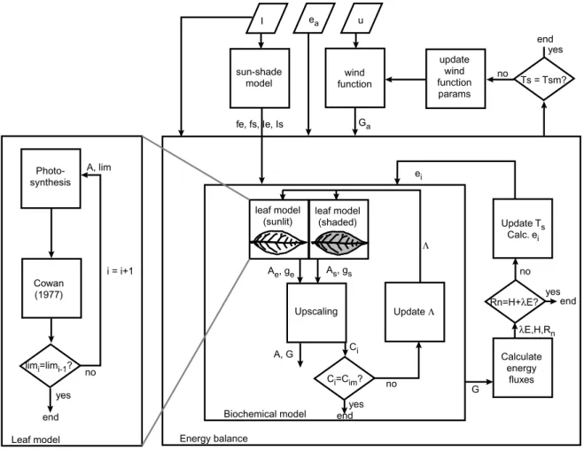
The model we used to calculate the fluxes of water and carbon dioxide consists of three components: photosynthesis and transpiration at leaf level as a function of biochemical pa-rameters, scaling of the fluxes to canopy level, and an energy balance of the canopy. At leaf level, diffusion equations, a biochemical model for photosynthesis (Farquhar et al., 1980) and the model for optimal stomatal control of Cowan (1977) are used. Scaling from leaf to canopy is carried out with a two-leaf model that distinguishes between a sunlit and a shaded fraction of leaves. An energy balance of the canopy is used to solve canopy temperature, which in turn affects the processes in the leaves. Figure 1 shows the structure of the model. In what follows, the three components of the model are presented.
Water and carbon dioxide move by diffusion in opposite directions between the stomata and the air. Water evaporates from the cell walls, and travels from the stomata to the air, whereas carbon dioxide travels from the air, via the stomata into the mesophyll, where it is reduced to sugars by the chem-ical reactions in the Calvin cycle. If the resistance for trans-port of carbon dioxide from the stomata to the mesophyll is neglected, then the diffusion equations can be written as: E=1.6gρa
Ma ei −ea
p =1.6gD (1)
A=g (Ca−Ci) (2)
whereEis evaporation andAassimilation (mol m−2s−1),g the effective aerodynamic and stomatal conductance (m s−1), ei andeathe vapour pressure in the intercellular spaces and in the ambient air (Pa), respectively,patmospheric pressure (Pa), ρa specific mass of air (kgm−3), Ma the molar mass of air (kg mol−1),D = ρa
Ma ei−ea
p the molar vapour concen-tration gradient between the intercellular space and the air (mol m−3), andCa andCi the molar carbon dioxide con-centration in the ambient air and in the stomata (mol m−3), respectively. The process of photosynthesis is described with the biochemical model of Farquhar et al. (1980). In this model, actual photosynthesis is the minimum of enzyme-limited and electron-enzyme-limited carboxylation, less dark respi-ration:
A= ν (Ci−Ŵ
∗)
Ci+γ −
Rd (3)
ν=Vcmandγ=Kc
1+O Ko
for Rubisco limited photosyn-thesis andν= qI Jm
4(I+2.1Jm) andγ=2Ŵ
∗for photon limited
Fig. 1. Flow chart of the combined photosynthesis-transpiration model. The enlargement at the left represents the biochemical model at leaf level.
oxygen concentration (mol m−3),KoandKc the Michaelis-Menten constants for carbon dioxide and oxygen (mol m−3), Rd dark respiration (mol m−2s−1),q the quantum yield ef-ficiency, Jm the maximum potential electron transport rate (mol m−2s−1) andIthe irradiance by photosynthetically ac-tive radiation (PAR) (mol m−2s−1).
Once values for the biochemical parameters are known, the diffusion equations (Eqs. 1 and 2) and the biochemical model (Eq. 3) form a set of three equations containing four unknowns (A,E,gandCi). A fourth equation, describing the stomatal behaviour, is required to yield a unique solution. Cowan (1977) and Cowan and Farquhar (1977) suggested that stomata operate such as to minimize the evaporative cost of plant carbon gain. This condition is met if the marginal water cost of assimilation3, is constant with time:
δE/δg
δA/δg =3= constant (4)
This model does not explain how stomatal regulation works physiologically, but only describes the stomatal behaviour that yields the highest mean assimilation rate over a time
pe-riod with variable environmental conditions, during which a certain positive amount of water evaporates. The parameter 3is a measure for the intrinsic water use (Lloyd and Far-quhar, 1994). Low values of3refer to more water efficient vegetation than high values. The advantage of this model for stomatal behaviour compared to empirical relations between stomatal conductance and humidity deficit, is that only one parameter, which has a conceptually clear meaning, is used. The model works best for the diurnal cycle, although it has also been applied to longer time periods, including dry condi-tions (Cowan, 1986). A problem with longer time scales and dry periods is that3does not remain constant (Makela et al., 1996; Arneth et al., 2002), because of hydraulic limitation of transport of water (Tyree and Sperry, 1988; Jones, 1998; Mencuccini, 2003) and because stomata respond to abscisic acid transmitted by roots (Zhang and Davies, 1989).
the case in which assimilation is enzyme limited and for the case in which assimilation is electron limited. Because it is not known a-priori whether assimilation is enzyme or elec-tron limited,Ci is solved by iteration of Eqs. (A1) to (A3) and the biochemical model (Eq. 3).
Climate variables in this model are photosynthetically ac-tive radiation (PAR), vapour pressure deficit and carbon diox-ide concentration. Biochemical parameters are maximum carboxylation capacityVcmand maximum electron transport Jm, quantum yield efficiencyq, marginal cost of assimila-tion3and Michaelis-Menten coefficients for the chemical reactions in the Calvin cycle.
The approach used to scale from leaf to canopy level (Ap-pendix B) is similar to that of De Pury and Farquhar (1997). Lambert-Beer’s equation is used to calculate the vertical dis-tribution of light in the canopy, discriminating between indi-rect (diffuse) and diindi-rect light, which have different extinction coefficients. Because the experimental sites were located on steep slopes, a coordinate rotation was used to correct for the effect of topography on the extinction coefficients for direct light (Appendix B). The model calculates the exposed and shaded fraction of leaves (fe andfs), and the intensities of PAR on the exposed and shaded leaves (IeandIs), which are variable over the day. The fluxes and the surface conductance at canopy level are calculated by adding the contributions of the two fractions:
V =L (feve+fsvs) (5)
whereV andv refer to any of the variablesA,Eandgat canopy and leaf level, respectively, the indexeto exposed andsto shaded, andLis leaf area index. The effective inter-nal carbon dioxide concentration for the canopy is:
Ci =Ca− A
G (6)
where A is canopy assimilation and G the canopy-scale equivalent ofg.
For the calculation ofEwith Eq. (1), an estimate of the internal vapour pressureei is needed, which cannot be mea-sured directly. The intercellular vapour pressure is in equilib-rium with leaf water potential and leaf temperature. Because air in stomata is always close to saturation, we assume that ei is the saturated vapour pressurees at surface temperature Ts:
ei =es(Ts) (7)
Surface temperature is solved from the energy balance. Ne-glecting soil heat flux and changes in heat storage, the energy balance is:
Rn=H+λE (8)
whereRn is net radiation, H sensible and λE latent heat flux (all in W m−2). Latent heat flux is calculated by con-verting E from units of mol m−2s−1 to kg m−2s−1 and
multiplying by the latent heat of vaporisation of water, λ (=2.501−0.0024T(◦C) MJ kg−1).
λE=1.6λρaGMH2O Ma
ei−ea
p (9)
whereMH2O the molar mass of water (kg mol−
1). Sensible
heat flux is calculated as:
H =ρacpGa(Ts−Ta) (10)
whereGathe aerodynamic conductance. Net radiation is calculated from incoming and outgoing shortwave and long-wave radiation:
Rn=(1−α)Rsi+Rli−Rlo (11) whereRsi,RliandRloincoming shortwave, incoming long-wave and outgoing longlong-wave radiation, respectively, andα the reflection coefficient for shortwave radiation (albedo). Outgoing longwave radiation is calculated with Stefan-Boltzman’s equation:
Rlo =εσ Ts4 (12)
whereε=0.98 the emissivity of the canopy and σ Stefan-Boltzman constant (=5.67×10⁻⁸W m−2K−4).
From the biochemical model (Eq. 1 to 4),A, E,Ci and gcan be solved, provided thatei is known. Equation (5) is used to scale from leaf to canopy, and from the energy bal-ance (Eqs. 7 to 12),ei,Tl,Rlo,Rn,HandλEcan be solved, provided thatGandGaare known. Both sub-models should be solved simultaneously. An analytical solution is not pos-sible due to the non-linearity of the interactions between the sub-models. For this reason, surface temperature is adjusted iteratively in order to force energy balance closure.
The aerodynamic conductance Ga is calculated with a wind function:
Ga=Ga0+Bu (13)
where Ga0 a convective term, u wind speed measured at
the meteorological station (m s−1), andBan empirical wind function. The termsGa0andBare calibrated by optimising
calculated surface temperaturesTs with measured ones. Be-causeTs is measured only at the south plot, the parameters Ga0andB of the south plot are also used at the other three
plots.
2.2 Site description
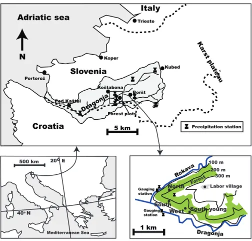
The study was part of a broader project to study the effects of natural reforestation on the water balance and geomorphol-ogy of the river catchment of the Dragonja River in Mediter-ranean Slovenia (N45◦28′E13◦46′, Fig. 2).
Fig. 2. Map showing the location of the four forest plots and meteorological stations.
to 1500 m high Karst plateaus form sharp orographic bound-aries at the north and the east with a more continental climate, with lower temperatures and higher precipitation. The Sub-Mediterranean climate is classified as Caf (mild winter, hot summer, no dry season) in the K¨oppen system. Mean annual precipitation varies from 1300 mm at the source to 1000 mm at the outlet of the Dragonja and is distributed evenly over the year.
The parent material in the Dragonja catchment is flysch: a sequence of calcareous shales and thin sandstone banks. In the upper part of the catchment, broad plateaus are in-tersected with narrow, steep river valleys of two contributing streams. In the lower part, the valley is broad and the plateaus narrow. The elevation ranges between 0 and 330 m above sea level. Soils in the whole catchment are Rendzina soils (Keesstra, 2006) and consist of clay loam (30 percent sand, 50 percent silt, 20 percent clay). Soil depth ranges from a few decimeters on the slopes to several meters of alluvial de-posits in the valley.
Four experimental plots were selected in deciduous forests, which contrasted in aspect, local hydrological and climate conditions and vegetation composition (Fig. 2). The forests had developed with minimum human interference
during the last 50 years. Both texture and chemical com-position of the soils at the plots were similar. One plot was located on a north and one on a south facing slope (north and south plot), and one at the foot of a converging west facing slope (west plot) and one with younger forest on a diverging south facing slope (south-young plot).
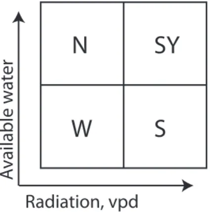
Relative differences in water availability, light, tempera-ture and vapour pressure deficit among the plots are pre-sented schematically in Fig. 3. Two plots were predomi-nantly sunlit and experience a high vapour pressure deficit, temperature and radiation input (south and south-young), and two plots predominantly shaded and experience a low vapour pressure deficit, temperature and radiation input (north and west). Two plots experience a high (north and south-young) and two plots a low (south and west) water availability. In this way, each of the four combinations of high and low vapour pressure deficit and high and low soil moisture con-tent was present.
Table 1.Characteristics of the four experimental forest plots in the Dragonja catchment.
north south west south-young
elevation (m) 180 190 120 150
slope 30◦ 30◦ 30◦ 30◦
aspect 330◦ 210◦ 270◦ 210◦
plot size (m2) 625 313 250 100
soil depth (m) 1.0 1.0 1.0 0.8
soil type clay loam clay loam clay loam clay loam
no of stems ha−1(103) 2.3 7.2 3.4 14.4
average diameter (cm) 12.8 7.3 8.6 4.0
average height (m) 16 8 14 4
mid-season LAI 4.0 5.2 4.5 2.7
age (y) >100 >100 >100 60
management (1900) wood gathering cattle grazing wood gathering crop field management (current) wood gathering wood gathering wood gathering wood gathering
Fig. 3. Schematic representation of relative differences in vapour pressure deficit and soil water availability the four forest plots: north (N), south (S), west (W) and south-young (SY).
Trees at the shaded plots were taller than at the sunlit plots. The forest at the south-young plot was younger, and pioneer vegetation was present (Juniperus communis).
2.3 Measurements
At each plot, vegetation and soil parameters, meteorologi-cal variables and the water balance were measured between May and September 2004. We selected only those data for which vegetation was not limited by water availability. The reason for doing so is that we are interested in the diurnal cy-cle during a period in which biochemical parameters remain constant, and water stress causes biochemical parameters to change in time (Lambers et al., 2000). Those temporal vari-ations of biochemical parameters in a changing environment are the subject of a study we will publish separately.
Basic meteorological variables (wind speed, diffuse and direct incoming shortwave radiation and reflected shortwave radiation) were measured at a meteorological station 3 km east of the experimental plots. Parameters for the biochemi-cal model at leaf level were derived from leaf chamber pho-tosynthesis measurements carried out on two species at the south and the south-young plot, and leaf nitrogen content and
13C isotope discrimination at all four plots.
Incoming and outgoing short wave and long wave radi-ation and net radiradi-ation were measured at one of the plots (south) with a CNR1 radiometer (Kipp and Zonen, Delft, Netherlands) mounted above the canopy. The temperature of the instrument itself was measured with a PT100 resis-tive temperature device. This setting provided accurate mea-surement of radiative temperature. In addition, radiative tem-perature was measured with a 4000.4ZH Everest radiometer (Everest Interscience, Inc.) Both instruments were pointed in NADIR. The radiative temperatures measured with the two instruments agreed very well, and only the data of the CNR1 radiometer were used in the analysis.
Temperature and relative humidity were measured at two m height with aspirated, shielded humicaps (HMP45AC, Vaisala Oyj, Finland), which were calibrated against a wet and dry bulb copper-constantan thermocouples (Vrije Uni-versiteit Amsterdam) before and after the study. Mean day-time temperature during the growing season was 22.8◦C, 23.9◦C, 21.4◦C and 24.3◦C for the north, south, west and south-young plot, respectively, and mean daytime vapour pressure deficit 11.0 hPa, 13.3 hPa, 9.6 hPa and 14.2 hPa for the same plots.
C
A F
Q o
north
J
F
Q o south−young
C
A F Q west
C A
F
S
Q o south
Carpinus betulus, orientalis
Acer campestre
Juniperus communis
Fraxunus ornus
Sorbus domesticus
Quercus cerris, pubescens, petrea
other
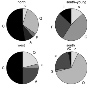
Fig. 4. Distribution of sap wood area over different species at the four forest plots.
south-young and the south plot between 14 and 21 July 2004. At the south-young plot, the trees were so small that mea-surements could be carried out at breast height. At the south plot, measurements were carried out on a scaffolding tower of 9 m height. The two species sampled are the most abun-dant species at the south and the south-young plot.
Leaf samples for analysis of carbon and nitrogen content and13C isotope discrimination were collected by a profes-sional tree climber at the start (a few weeks after bud break) and the end (four weeks before the onset of senescence) of the growing season at all four plots. The total number of leaf samples was 83 (15 at the north, 31 at the south, 16 at the west and 21 at the south-young plot). One third of the sam-ples was collected between 5 May and 8 June 2004, and two third between 8 and 10 September 2004. Each sample con-sisted of 4 to 15 leaves of different size from neighbouring branches of a tree. The number of samples of a species was chosen such that it approximated the relative contribution to the total sapwood area of that species at the plot. Species which contributed less than 5 percent to the total sapwood area were not sampled. At all plots, the sampled species rep-resented over 85 percent of the sapwood area. Leaves were collected both high in the canopy (predominantly sunlit) and low in the canopy (predominantly shaded). Samples were classified by plot, species, sunlit or shaded, and young or old leaves.
The leaves were air dried, oven dried at 50◦C, minced in a mincing machine and grounded in centrifugal ball mill. Carbon and nitrogen content (percentage by weight) and discrimination of 13C were determined using an elemental CHNO-analyzer Flash EA 1112 (Finnegan MAT, Bremen, Germany).
The13C discrimination against ambient air was calculated
as (Farquhar and Richards, 1984): 113Cl =
δ13Ca−δ13Cl 1+113C
l
(14) whereδ13C the isotope ratio per mil compared to the PDB standard, subscriptaandlindicate air and leaf, respectively, andδ13Ca=−8 ppm. The long-term internal carbon dioxide concentration was calculated as (Farquhar et al., 1989):
Ci Ca =
113Cl−c1
c2−c1
(15) wherec1=4.4 per mil the discrimination by diffusion in air
andc2=27 per mil the discrimination by Rubisco.
The leaf samples were used to calculate effective values for leaf nitrogen content and13C isotope discrimination for each plot. First, a Kolmogorov-Smirnov test showed that the measurements of leaf nitrogen and13C within each plot had normal distributions, and a Levene test showed the variances within the plots were not different from each other. Next, the estimated mean valuesmˆ and variancessˆ2for each plot were calculated as:
ˆ m=X
ns
Fim (16)
ˆ s2=X
ns
Fi2sˆi2 (17)
whereFi the contribution of speciesito total sapwood area, andns the number of sampled trees of speciesi. A 95% confidence interval for the mean was calculated as:
m= ˆm±s0.95
s ˆ s2
where s0.95 the Student-t statistic for p=0.95 and np the number of samples at each plot.
The parameters for the model of Farquhar and internal car-bon dioxide concentration for each plot were derived in the following way. First, maximum carboxylation capacity and electron transport capacity for each plot were calculated by fitting the Farquhar model to the leaf chamber photosynthe-sis measurements. Next, a linear relationship between max-imum carboxylation capacity and leaf nitrogen content was fitted for the leaves for which measurements of both leaf ni-trogen content and maximum carboxylation capacity were available. Finally, this linear relationship was used to derive values for the maximum carboxylation capacity at all four plots from measurements of leaf nitrogen content. Leaf ni-trogen content did not change significantly between the start and the end of the season, whereas the light response curves changed and the parameters Vcm andJm dropped after the onset of drought (not shown).
The average values of internal carbon dioxide concentra-tionCi¯ from the isotope analysis were used to calibrate the model parameter3for each plot, by minimising the abso-lute difference between measured and calculated internal car-bon dioxide concentration. Modelled internal carcar-bon dioxide concentration changes during the day. An average was cal-culated by weighingCiwith the instantaneous rate of photo-synthesis (Farquhar et al., 1982):
¯ Ci =
Z A(t )C i(t ) ¯
A dt (19)
Temperature, relative humidity, vertical profiles of soil moisture content and sap flux density were measured con-tinuously at each plot, and data stored at 30-min intervals. Precipitation was measured at 3 stations within 500 m of the forest plots. Transpiration was calculated from sap flux den-sity measurements with the method of Granier (1987). At each plot, 12 sensors were installed in 6 trees (2 sensors per tree). The trees were selected such that they best represented the distribution of species and stem diameters (Fig. 4). From each of the three most abundant species at each plot, at least one tree was sampled. Fraxinus ornus was sampled at all four plots because it was present at all plots, and either Quer-cus pubescensorQuercus cerriswas sampled at each plot. Both ring porous (QuercusandFraxinus ornus) and diffuse porous species (Carpinus betulus,Juniperus communisand Acer campestre) were sampled.
Effective mean sap flux density and a 95% confidence in-terval were calculated from the individual sensors weighed by the contribution of each species to the total sapwood area, in the same way as for leaf nitrogen (Eq. 16 to 18). La-tent heat flux, λE (W m−2), was calculated by multiply-ing sap flux density by the area of sapwood per unit forest floor fA and by the latent heat of vaporization of water λ (2.5 MJ kg−1):
λE=λfAm (20)
The area of sapwood per unit forest floor,fA, was calculated in the following way. Because the sensors had a length of 20 mm and were inserted in heat-conducting material, it was assumed that the measured sap flux density is the effective sap flux density of the outer 20 mm of the stem. If sapwood area extends deeper than 20 mm into the stem, then the sap flux measurements are underestimates. For this reason, the actual sapwood area was inferred from microscopic analy-sis of tree cores taken perpendicular to the tree rings of all sampled trees at the end of the growing season of 2004. A film of approximately 0.1 mm thickness was planed off the tree cores with a razor blade and examined visually under a microscope for the presence of active xylem vessels. The ma-jority of xylem vessels were present in the outer 20 mm, and few extended up to 40 mm depth. The number of sampled trees (24) was too small to establish a relationship between sapwood area, species and plot. Because only 10 to 30% of active xylem vessels were present at depths greater than 20 mm, we used a value of 25 mm±10% for the sapwood depths for all trees at all plots. The total sapwood area per unit forest floor was calculated by measuring the diameters of all trees in each plot.
It is noteworthy that leaf nitrogen content and isotope dis-crimination were calculated as averages from leaf samples weighed with the relative contribution of species to total sap-wood area (Eq. 16), whereas latent heat was calculated by multiplying sap flux density with the absolute values of sap-wood area (Eq. 20). Latent heat flux is therefore sensitive to errors in sapwood area, and leaf nitrogen content and isotope discrimination only to errors in the relative contribution of each species.
Table 2.A-priori parameter values for the biochemical model. (Farquhar et al., 1980)
Kc(mmolm−3) Ko(mbar) O(mbar) Ŵ∗(mmolm−3) Jm/Vcm
18.7 330 210 1.22 2.5
Table 3.Fitted values of maximum carboxylation capacityVcm, dark respiration rateRdand quantum yield efficiencyqwith 0.95-confidence
intervals, fitted for measurements on 13 leaves ofQuercus pubescensand 6 leaves ofFraxinus ornusat the south and the south-young plot between 14 and 21 July 2004.
Vcm(µmolm−2s−1) Rd(µmolm−2s−1) q
Quercus pubescens 54±9 1.0±0.2 0.46±0.15 Fraxinus ornus 44±7 1.1±0.0 0.39±0.09
3 Results
In this section we present the derivation of the parameters for the biochemical model at leaf level from leaf chamber pho-tosynthesis measurements and leaf samples, the validation of the sun-shade model, the model predictions of diurnal cycles of the fluxes. The discussion section is dedicated to a sensi-tivity analysis of the model.
3.1 Biochemical model
Figure 5 shows leaf chamber photosynthesis measurements used for parametrization of the biochemical model, and model predictions (solid lines). The upper panels show net assimilation as a function of photosynthetically active radia-tion (PAR), the lower panelsCi/Caversus PAR. The param-etersVcm,Rd andq of the photosynthesis model were fitted (Table 3) using these data, whereas a-priori values were used for other parameters (Table 2). The measurements were car-ried out at similar vapour pressure deficit (10 hPa, controlled) and temperature (28±2◦C, not controlled).
The measured values of maximum photosynthesis rate of Quercus pubescens agree with measurements of Damesin and Rambal (1995), who found values of 10.0 to 16.5 µmol m−2s−1 in a Mediterranean climate. If the hy-pothesis of Cowan (1977) holds, then Ci should be inde-pendent of PAR. However, Fig. 5 shows a sharp increase ofCi/Ca when PAR decreases to low values (Ca remained constant during these measurements). This is either caused by a minimum stomatal conductance that prevents the stom-ata to fully close, or by the fact that the time interval of 2 min between the measurements was too short for the stom-ata to reach an equilibrium. The first possibility implies that the model of Cowan (1977) is incomplete. The solid line in Fig. 5 was derived by assuming a relation between as-similation and stomatal conductance as proposed by Leun-ing (1995). In the analysis that follow the model of Cowan (1977) is used, because its parameter3has a conceptually clear meaning.
The values forVcmfor the two sampled species (Table 3) were used to fit the linear relationship between leaf nitrogen content andVcm. Unfortunately, a direct translation from leaf nitrogen content to photosynthetic capacity is not possible, because leaf nitrogen content measurement were based on samples of multiple leaves, whereasVcmwas calculated for individual leaves. Because of limited access to the canopy, leaf photosynthesis could not be measured for all species and not always for the same leaves as leaf photosynthesis. Ide-ally, data of all species should be used, and the relationship evaluated per species. Correlating leaf nitrogen content and photosynthetic capacity is a simplification, because the ef-fects of leaf thickness and density are not considered. In spite of these simplifications, there is evidence that leaf nitrogen content is positively related to photosynthetic capacity and maximum photosynthesis, even across different genotypes (Reich et al., 1999). Niinemets (1999) found a linear positive relationship between photosynthetic capacity (calculated by inverting the model of Farquhar) and leaf nitrogen content per unit dry mass among a large number of C3 species on earth. Figure 6 shows leaf nitrogen versusVcm for the two sampled species at the south and the south-young plot, with 0.95 confidence intervals for both nitrogen content andVcm. We adopt a linear relation of Field and Mooney (1986) to relateVcmto nitrogen content:
Vcm=x(N−N0) (21)
whereN0the residual leaf nitrogen content (=25 mmol m−2
0 0.5 1 1.5 2 0
4 8 12 16
A n
(
µ
mol m
−2
s
−1
)
Quercus pubescens
0 0.5 1 1.5 2
0.6 0.7 0.8 0.9 1 1.1
I
PAR (mmol m
−2 s−1)
C i
/C
a
0 0.5 1 1.5 2
0 4 8 12 16
Fraxinus ornus
0 0.5 1 1.5 2
0.6 0.7 0.8 0.9 1 1.1
I
PAR (mmol m
−2 s−1)
Fig. 5. Rates of net photosynthesis (µmol m−2s−1) (upper panels), andCi/Cs versus intensity of photosynthetically active radiation PAR
(mmol m−2s−1) (lower panels) forQuercus pubescensandFraxinus ornus. Measurements were carried out at the south and the south-young plot between 14 and 21 July 2004. The solid line is a prediction of the fitted biochemical model. For the lines in the lower panels, the model of Leuning (1995) was used.
0.6 0.8 1 1.2 1.4 1.6
0 10 20 30 40 50 60 70 80
Quercus p.
Fraxinus o.
N (g / 100 g DM−1)
V cm
(
µ
mol m
−2
s
−1
)
Fig. 6. Mean maximum carboxylation capacityVcm, with
0.95-confidence intervals for Quercus pubescens and Fraxinus ornus, versus mean leaf nitrogen with 0.95-confidence intervals, measured at the south and the south-young plot, and a linear regression line through the two data points, forced throughVcm(0.5)=0. Dots
re-fer measurements by Reich et al. (1999) between N=0 and N=1.7 g (100 g DM)−1, and were calculated with Eq. (3) from light satu-rated photosynthesis, assumingCi=0.7Caand using the constants
of Table 2 and a quantum yield efficiencyqof 0.45.
Table 4 shows the biochemical parameters as derived from the leaf sample analysis and leaf photosynthesis measure-ments, and leaf area index for the four plots. ForRd and q, we used equal values for all plots. Differences in nitrogen content between sunlit and shaded leaves were not signifi-cant, perhaps due to the open structure of the canopy. It is remarkable that the two plots with the lowest vapour pres-sure deficit (north and west) have higher carboxylation ca-pacityVcm than the two plots with the highest vapour pres-sure deficit (south and south-young), and that the two plots with the lowest soil moisture content (south and west) have a higher intrinsic water use efficiency (lower3) than the two plots with a higher soil moisture content. This topic will be discussed in detail in a separate study which focusses on the relation between climate and biochemical parameters. 3.2 Sun-shade model
Figure 7 shows the modelled versus the measured fraction of direct light that reaches the forest floorI /I0at the north and
Table 4.Mean values of leaf nitrogen concentration [N] and13C isotope discrimination with 95% confidence intervals, maximum carboxy-lation capacityVcm, dark respirationRd, marginal cost of assimilation3, quantum yield efficiencyq, and leaf area indexLat the north,
south, west and south-young plot.Vcmwas derived from leaf nitrogen concentration and leaf chamber measurements,3from13C isotope
discrimination,qandRdfrom leaf chamber measurements andLfrom PAR measurements.
north south west south-young
[N](g 100g−1) 1.61±0.08 1.33±0.03 1.74±0.16 1.34±0.04 113C (ppm) 21.20±0.24 19.95±0.31 19.76±0.21 20.73±0.22 Vcm(µmol m−2s−1) 68 51 70 52
3 1233 622 507 1030
Rd(µmol m−2s−1) 1.0 1.0 1.0 1.0
q 0.45 0.45 0.45 0.45
L 3.9 4.4 4.2 2.5
vertical profiles of measured (x) and modelled (line) light distribution in the canopy at the south plot, measured at dif-ferent times of the day and for difdif-ferent weather conditions. The depth is in units of leaf area index, assuming a homo-geneous leaf distribution over depth. From left to right and from top to bottom, the fraction of diffuse ambient irradiance increases from 13 to 100%. The curves are similar in shape, and the model performs well in all conditions except for low solar angles and low light intensity (lower left and lower mid-dle panel). Although the shape of the curves are similar, large differences exist in the irradiance on sunlit and shaded leaves depending on light conditions and time of the day. The in-sets show calculated values for the fractions of sunlit (open boxes) and shaded (shaded boxes) leaves, and the mean in-tensities of PAR on sunlit and shaded leaves. With increasing fraction of indirect radiation, the difference in irradiance be-tween sunlit and shaded leaves decreases.
3.3 Diurnal cycle of assimilation and latent heat
Figure 9 shows the mean diurnal cycles ofA, λE andGs for all 20 clear days between 29 May and 8 July 2004. Dur-ing this period, the time of sunrise and sunset shifted by ap-proximately 14 min. Because this is smaller than the time resolution of the data (30 min), no correction was made for this. The lines are model predictions, the bars 0.95 confi-dence intervals for latent heat flux estimated from sap flux measurements (from now on referred to as measured latent heat), and surface conductance calculated from measured la-tent heat using the inverse Penman-Monteith equation.
The diurnal cycles of assimilation show some typical fea-tures which can be explained from biochemical properties and environmental conditions. The increase of assimilation in the morning and the decrease in the evening are slower at the north and the west than at the south and the south-young plot. This can be attributed to the lower fraction of sunlit leaves at the north and the west plot than at the south and the south-young plot, and consequently a greater contribution of leaves that assimilate at a light limited rate, even late in the
0 0.02 0.04 0.06 0.08 0.1
0 0.02 0.04 0.06 0.08 0.1
I / I
0 (meas)
I
/
I 0
(mod)
north
south
Fig. 7. Modelled versus measured fraction of ambient PAR that reaches the forest floor, for different weather conditions and differ-ent times of the day (6 to 19 h) at the north and the south plot, for different days between May and September 2004. The values in the circle refer to low-light conditions in the late afternoon.
morning. Although assimilation reaches its peak later at the north and the west plot than at the south and the south-young plot, the peak values are higher due to a higher value of max-imum carboxylation capacityVcm.
0 2 4 0
0.5 1
15−May−2004 16:07
I /
I 0
0 0.5 1 0 1 2
fe, fs
I (mmol m
−2
s
−1
)
0 2 4
0 0.5 1
31−May−2004 10:30
0 0.5 1 0 1 2
0 2 4
0 0.5 1
07−Jun−2004 14:30
0 0.5 1 0 1 2
0 2 4
0 0.5 1
15−May−2004 17:30
depth in canopy (units LAI)
I /
I 0
0 0.5 1 0 1 2
0 2 4
0 0.5 1
07−Jun−2004 17:15
depth in canopy (units LAI) 0 0.5 1 0 1 2
0 2 4
0 0.5 1
04−Jun−2004 12:10
depth in canopy (units LAI) 0 0.5 1 0 1 2
Fig. 8. Measured (x) and modelled (lines) vertical profiles of light intensity relative to ambient light (I /I0) for different weather conditions at the south plot on different days in May and June 2004. The insets indicate the difference between sunlit and shaded leaves: the open boxes refer to the sunlit fraction, the shaded boxes to the shaded fraction. The width of the boxes denotes the size of the fraction, and the height the intensity of PAR. From left to right and from top to bottom, the fraction of diffuse ambient irradiance increases from 13 to 100%.
and therefore a lower latent heat flux than the north plot. The south and the south-young plot both have a relatively low Vcm, but the south-young plot has a higher3and therefore a higher latent heat flux than the south plot.
The model accurately reproduces the diurnal cycles of sur-face conductance derived from the inverse Penman-Monteith equation. The north plot does not show afternoon stomatal closure, whereas the other three plots show a typical pattern of stomatal closure in the late morning and afternoon. This can be explained by the combined effects of vapour pressure deficit and the parameter3. Low values of3(low marginal cost of assimilation) indicate early stomatal closure in re-sponse to vapour pressure deficit, whereas high values of3 indicate that stomata remain open relatively long. The values for3are lower at the two plots with low water availability (south and west plot) than at the two plots with high water availability (north and south-young plot). Whether afternoon stomatal closure occurs is then indicated by the schematic representation of the plots in Fig. 3. At the north plot, stom-ata remain open because both 3 is high and vapour pres-sure deficit low, whereas at all other plots,3is low, stomatal deficits are high, or both. At south plot,3is low and vapour pressure deficit high, at the west plot, 3is low, and at the south-young plot, vapour pressure deficit high. For all four plots, the modelled diurnal cycles agree with those derived from the inverse Penman-Monteith equation, which shows
that measurements of leaf biochemistry and climate contions together can be used successfully to reproduce the di-urnal cycles of stomatal conductance, and to distinguish be-tween the effects of biochemistry and climate.
In Fig. 10, the data are presented in a different way. This figure shows modelled versus measured latent heat flux for all half-hourly data between 29 May and 8 July 2004. The solid lines are 1:1 lines. For all plots, the squared correlation coefficients are above 0.90. Latent heat flux at the north plot is slightly underestimated, and maximum latent heat flux at the south and south-young plot overestimated. The signifi-cance of this difference between measured and modelled la-tent heat flux is discussed in the next section using an error propagation analysis of the model. The relationship between modelled and measured latent heat flux is slightly convex, especially at the north and south slope. A closer look at the diurnal cycles shows that this effect is caused by the fact that sap flux continues for some time after sunset, and most likely lags behind latent heat flux in the afternoon. This aspect is discussed in the next section as well.
0 10 20 30
A (
µ
mol m
−2
s
−1
)
north
0 100 200 300
λ
E (W m
−2
)
6 9 12 15 18
0 5 10
G s
(mm s
−1
)
time (hours) 0 10 20 30
south−young
0 100 200 300
6 9 12 15 18
0 5 10
time (hours) 0 10 20 30
west
0 100 200 300
6 9 12 15 18
0 5 10
time (hours) 0 10 20 30
south
0 100 200 300
6 9 12 15 18
0 5 10
time (hours)
Fig. 9. Modelled rates of net photosynthesis (µmol m−2s−1), latent heat fluxλE(W m−2), and surface conductanceGs (mm s−1) at the
north, south, west and south-young plot for 20 clear days between 29 May and 8 July 2004. Lines are model predictions, and bars latent heat flux and surface conductance derived from independent sap flux measurements, and 95% confidence intervals, derived from measurements of 12 sap flux sensors per plot. Bars for surface conductance were derived by inverting the Penman-Monteith equation, using the sap-flux based estimates of latent heat flux.
0 100 200 300 400
0 100 200 300 400
λE
meas (W m −2
) south
r2 = 0.92 1:1
south 1:1
0 100 200 300 400
0 100 200 300 400
λ
E mod
(W m
−2
) north
r2 = 0.92 1:1
0 100 200 300 400
0 100 200 300 400
south−young
r2 = 0.93 1:1
0 100 200 300 400
0 100 200 300 400
λE
meas (W m −2
)
λ
E mod
(W m
−2
) west
r2 = 0.93 1:1
Table 5. Sensitivity of assimilationAand latent heatλEto pa-rameter or variablex with standard deviationσx, calculated with
Eq. (22). Standard deviation are also expressed as percentage of the mean values of assimilation and latent heat.
x σx σA σλE
µmolm−2s−1 % Wm−2 %
D 3 hPa 0.30 5 4.0 5
Vcm 10µmol m−2s−1 0.72 12 7.2 10
3 100 0.27 4 5.8 8
L 0.5 0.64 11 6.5 9
total 1.05 13 12 11
difference between surface temperature and air temperature at the south plot (left panel), and the modelled temperature difference versus the measured temperature difference for all half hourly values between 19 May and 8 July 2004 (right panel). The correlation between modelled and measured sur-face temperature is lower than that for latent heat. This is a minor problem, becauseTs−Tais relatively small compared to the diurnal cycle ofTa, and the model prediction of latent heat is not very sensitive to errors inTs−Ta. The difference between the model and measurements could be related to a hot-spot effect in the radiative temperature measurements.
4 Discussion
The agreement between modelled and measured fluxes de-pends on the accuracy of four components: (1) measure-ments used for validation, (2) input variables, (3) parameter values and (4) the model description itself.
The uncertainty in the measurements for validation in-cludes the variation of sap flux density measurements among sensors and the sapwood-surface area ratio. An additional er-ror is that we ignored the time lag that exists between transpi-ration and sap flux due to storage of water in stems (Schulze et al., 1985). The data indicate that indeed for some time after sunset, sap flow continues. However, there is no reason why storage in stems and the time lag would be equal for all four plots (tree heights vary from 3 m at the south-young plot to 18 m at the north plot). To account for the time lag requires at least four additional parameters to be estimated (one for each plot). To calibrate these parameters against modelled latent heat would compromise our aim to use independent data for validation of the model. An alternative would be to use radiation data to estimate the time lag, but doing so also creates a dependence between the model and the validation data, because the same radiation data are also used as input in the model. Any other parametrization would be highly subjective. For this reason, we did not account for the time lag.
The sensitivity of the model to the most relevant input variables and parameters was calculated with an error prop-agation analysis, assuming all errors were uncorrelated. The variance of the model predictionσy2of an output variabley can be calculated from the variances of the variables and pa-rametersxas:
σy2=X i
σx2 δy
δx 2
(22) The greatest uncertainty in the input variables is the vapour pressure deficit, which was measured at 2 m height rather than in or above the canopy. For four weeks at the end of the growing season in 2004, the instrument for temperature and relative humidity was moved to just above the canopy at 9 m height at the south plot. A comparison with mea-surements before and after relocation of the instrument with data of the other plots showed that both temperature and rel-ative humidity are lower above than below the canopy. The net effect was that vapour pressure deficit was<2 hPa higher above than below the canopy. At the north and the west plot, the effect might have been larger because of the taller trees and the denser canopy. In the sensitivity study, we assumed σes−e=3 hPa. The greatest uncertainty in the biochemical pa-rameters is the maximum carboxylation capacityVcm. The accuracy ofVcm depends on the accuracy of nitrogen mea-surements and the relation with leaf chamber photosynthesis measurements. Based on the confidence intervals of nitro-gen and leaf chamber photosynthesis measurements and the coarse relationship between nitrogen content and Vcm, we assumedσVcm=10µmol m−2s−1, which is about 20% of the actual values.
Table 5 shows the sensitivity of the mean value of the fluxes of water and carbon dioxide to variations in es−e, Vcm, 3 andL, absolute and as a percentage of the actual values. In the table we present standard deviations instead of variances. The difference between modelled and measured latent heat flux (Fig. 9) is smaller than the standard devia-tion of the error of the model predicdevia-tion, i.e. the difference between modelled and measured latent heat falls within the accuracy of the parameter values and input variables. Thus, there is no reason to improve the accuracy of the physical model description itself. The uncertainty of the vapour pres-sure alone is insufficient to explain the difference between measured and modelled latent heat flux.
0 6 12 18 0 −0.5
0 0.5 1 1.5 2 2.5 3 3.5
time (hrs) T s
−T
a
(
° C)
−1 0 1 2 3 4
−1 0 1 2 3 4
T
s meas−Ta (
°C) T s mod
−T
a
(
° C)
r2 = 0.53
Fig. 11. Diurnal cycle of the measured (x) and modelled (line) difference between surface and air temperature at the south plot on 27 June 2004 (left), and the modelled versus the measured difference between surface and air temperature for half hourly values between 29 May and 8 July 2004 (right).
the fine line is the model where vapour pressure deficit, tem-perature, incoming radiation and aspect have been reversed, and the dashed line the model where parametersVcm,Jmand 3have been reversed. Reversing the parameters has a greater effect on surface conductance than reversing the meteorolog-ical variables. Reversing the biochemmeteorolog-ical parameters results in a large change of the magnitude of surface conductance, but a similar shape of the diurnal cycle. Reversing the me-teorological variables also changes the shape of the diurnal cycle, especially the hour of the peak.
Wilson et al. (2003) studied the time lag between the peaks of radiation and the fluxes of carbon and latent heat for differ-ent climates. The time lag between the the peak of radiation and surface conductance we find is for the south plot simi-lar to what they found for Mediterranean forests, and for the north plot similar to what they found for boreal forests. Our results indicate that this difference is mainly caused by the diurnal cycles of radiation, temperature and vapour pressure deficit.
The large effect of the spatial variations of biochemical parameters on the fluxes suggests that models which use uni-form biochemical parameters would not predict the observed spatial variability of the fluxes. If average biochemical pa-rameters are used for the north and the south plot, then sur-face conductance is overestimated at the south plot and un-derestimated at the north plot.
Although we demonstrated that spatial variations in bio-chemical parameters are important, we did not address the questions why biochemical parameters vary among the plots the way they do, and whether we can predict spatial patterns. Biochemical parameters are functions of environmental con-ditions: water potentials in soil and air, the availability of
wa-ter and nutrients and temporal variations therein, and stand age, succession, pests and diseases and anthropogenic influ-ence. A model to explain biochemical parameters from long term climate will be the subject of a separate study.
5 Conclusions
This study showed that both the magnitude and the shape of the diurnal cycle of transpiration and stomatal conduc-tance can be calculated from measurements of leaf nitrogen,
13C isotope discrimination and leaf photosynthesis
measure-ments. Although the data, due to uncertainty in photosyn-thetic capacity, do not allow for an exact quantification, a sensitivity analysis showed that the diurnal cycles were more strongly affected by spatial variations in vegetation param-eters than by meteorological variables. This indicates that topography induced variations in vegetation parameters are of at least equal importance for the fluxes as topography in-duced variations in radiation, humidity and temperature.
Appendix A
Cowan-Farquhar model after Arneth et al. (2002)
6 9 12 15 18 0
2 4 6 8
G s
(mm s
−1
)
north
time (hours) north north
6 9 12 15 18
0 2 4 6
8 south
time (hours) south south
Fig. 12. Modelled and measured surface conductance for the north and the south plot, as in Fig. 9 (bold line), modelled surface conductance after reversing aspect, radiation, temperature and vapour pressure deficit of the north and south plot (fine line), and after reversingVcm,Jm
and3of the north and south plot (dashed line).
Fig. 13. Definition sketch of the zenith angleθ, the angle of the surface in the plane of the direct light beamφ′, and the modified zenith angleθ′for sloped terrain.
and one for electron limited photosynthesis. In both cases, the equation forCi is quadratic:
k2Ci2+k1Ci+k0=0 (A1)
where
k2=3+
1.6D k′+Ŵ∗ k1=1.6D−2Ca3+
1.6D(Ŵ∗−k′) k′+Ŵ∗
k0=(3Ca−1.6D)Ca+
1.6DŴ∗k′ k′+Ŵ∗
k′=Kc(1+O/Ko) (A2)
for the enzyme limited case and k2=3−
1.6D 3Ŵ∗
k1=1.6D−2Ca3+
1.6DŴ∗ 3Ŵ∗
k0=(3Ca−1.6D)Ca+
1.6D2Ŵ∗2
3Ŵ∗ (A3)
for the electron limited case.
Appendix B
Light distribution model
The extinction of both indirect and direct light in a canopy is calculated analogous to light absorption in homogeneous media with the law of Lambert-Beer:
I (l) I0 =
exp−κI (B1)
whereI light intensity,lthe depth in the canopy in units of Lfrom the top of the canopy andκan extinction coefficient, which depends on the zenith angle of the light beamθ and the orientation of the leaves. The orientation of the leaves is expressed by the ellipsoidal leaf angle distribution parameter x, wherex<1 for mainly vertical leaves,x=1 for a spherical leaf distribution orx>1 for mainly horizontal leaves. The extinction coefficientκis (Campbell, 1986):
κ(x, θ )=
p
x2+tan2(θ )2
x+1/ (2ǫ1x)ln[(1+ǫ1)/(1−ǫ1)]
if x >1
κ(x, θ )=κ =px2+tan2(θ )2 ifx=1
κ(x, θ )= p
x2+tan2(θ )2
x+arcsin(ǫ2)/ǫ2
if x <1 (B2)
whereǫ1=
p
1−1/x2andǫ 2=
The extinction coefficients for indirect and direct light are different, because they origin from a different directions. The calculation of the extinction of direct light is straightforward, but the extinction of indirect light must be calculated by in-tegration of Eq. (B1) and (B2) over the sky area. In practice, this results in an extinction coefficient of 0.7 ifx=1, inde-pendent of geographical location, time of the year or time of the day.
In terrains of steep topography, the penetration of direct light into the canopy is different from that in flat areas. To include the effect of topography, a modified zenith angle is used in Eq. (B2). The coordinate system is rotated such that the surface becomes horizontal, and the zenith angle is cal-culated for the rotated coordinate system. A sloped surface is described by its steepest angle φ and the orientation of the slopeω, which is the horizontal direction of the steepest downward slope, measured clockwise from north. The angle of the surface in the plane of the direct light beam and the verticalφ′, is defined as (Fig. 13):
φ′=arctan(tan(φ)cos(ωs−ω)) (B3)
whereωsthe hour angle of the sun. The rotated zenith angle,
θ′, is defined as the angle between the vector perpendicular to the slope and the solar beam, i.e.:
θ′=θ+φ′ (B4)
In the calculation of the vertical profile of light in the canopy with Eqs. (B1) and (B2),θ′ is used instead ofθ. By doing so, it is implicitly assumed that leaf angle distributionx is unaffected by the coordinate rotation. This is an acceptable assumption if leaf angle distribution is spherical, but may not be acceptable if leaf angle distribution is strongly erectophile or planophile. In this study, it is assumed thatx=1.
It is assumed that leaves are either sunlit or shaded. The effect of a partial eclipse due to the fact that direct radiation does not origin from a point source, or due to light bending over edges of leaves, is ignored. Sunlit leaves receive direct and diffuse light, shaded leaves receive only diffuse light. Scattering and transmission of direct light is ignored, and it is assumed that reflected direct light does not meet other leaves on its way back to the atmosphere. The fractions of sunlit leavesfe, and shaded leavesfs, are functions of depth in the
canopylin units of leaf area index: fe(l)=
Id(l)
Id0
(B5)
fs=1−fe (B6)
whereId0the intensity of ambient direct light. The intensities
of irradiance on the two fractions are:
Ie(l)=Id0+Ii(l) (B7)
Is(l)=Ii(l) (B8)
Total light intensity at depthlin the canopy is:
I (l)=feIe(l)+fsIs(l)=Ii(l)+Id(l) (B9)
The exposed and shaded fractions and the irradiance on the fractions for the whole canopy are calculated by integrating Eqs. (B5) to (B8) over the leaf area index. In this study, the integration was done numerically using intervals of units leaf area index of 0.1.
Acknowledgements. The authors thank J. de Lange, R. Lootens, K. de Bruine and H. Visch of the Vrije Universiteit (VU) for devel-oping the sapflow sensors and other equipment, M. Groen (VU) for his technical support, M. Hooyen, S. Verdegaal, M. Konert, H. Vonhof and N. Slimmen (VU) for laboratory analyses, F. Batic of the Universitity of Ljubljana (Lj), R. Aerts and P. van Bodegom (VU) for allowing me to use their equipment, L. Globevnik of the institute for Water in Ljubljana for her administrative support, V. Zupanc and M. Padenik (Lj) for their work in the field, Peter for climbing the trees, and the reviewers for their useful comments.
Edited by: T. Laurila
References
Arneth, A., Lloyd, J., ˇSantr˙uˇckov´a, H., Bird, M., Grigoryev, S., Kalschnikov, Y., Gleixner, G., and Schulze, E.-D.: Response of central Siberian Scots pine to soil water deficit and long-term trends in atmospheric CO2concentration, Global Biochem. Cy-cles, 16, 5/1–5/13, doi:10.1029/2000GB001374, 2002.
Campbell, G.: Extinction coefficients for radiation in plant canopies calculated using an ellipsoidal inclination angle distribution, Agric. For. Meteorol., 36, 317–321, 1986.
Cowan, I.: Stomatal behaviour and environment, Adv. Bot. Res., 4, 117–228, 1977.
Cowan, I.: Economics of carbon fixation in higher plants, in: On the economy of plant form and function, edited by: Givnish, T. J., Cambridge University Press, Cambridge, UK, pp. 133–170, 1986.
Cowan, I. and Farquhar, G.: Stomatal function in relation to leaf metabolism and environment, Soc. Exp. Biol. Symp., 31, 471– 505, 1977.
Damesin, C. and Rambal, S.: Field study of leaf photosynthetic performance by a Mediterranean deciduous oak tree (Quercus pubescens) during a severe summer drought, New Phytol., 131, 159–167, doi:10.1111/j.1469-8137.1995.tb05717.x, 1995. De Pury, D. and Farquhar, G.: Simple scaling of photosynthesis
from leaves to canopies without the errors of big-leave models, Plant Cell Environ., 20, 237–557, 1997.
Farquhar, G. and Richards, R.: Isotopic composition of plant carbon correlates with water-use efficiency of what genotypes, Austr. J. Plant Physiol., 11, 191–210, 1984.
Farquhar, G. and Sharkey, T.: Stomatal Conductance and Photo-synthesis, Ann. Rev. Plant. Physiol., 33, 317–345, doi:10.1146/ annurev.pp.33.060182.001533, 1982.
Farquhar, G., O’Leary, M., and Berry, J.: On the relationship be-tween carbon isotope discrimination and the intercellular carbon dioxide concentration in leaves, Austr. J. Plant Physiol., 9, 121– 137, 1982.
Farquhar, G., Ehleringer, J., and Hubick, K.: Carbon isotope dis-crimination and photosynthesis, Annu. Rev. Plant Physiol. Plant Mol. Biol., 40, 503–537, 1989.
Field, C. and Mooney, H.: The photosynthesis-nitrogen relation-ship in wild plants, in: On the Economy of Plant Form and Func-tion, edited by: Givnish, T. J., Cambridge University Press, Cam-bridge, UK, pp. 25–55, 1986.
Granier, A.: Mesure du flux de s`eve brute dans le tronc du Douglas par une nouvelle m´ethode thermique, Ann. Sci. Forest, 44, 1–14, 1987.
Harley, P. and Baldocchi, D.: Scaling carbon dioxide and water vapour exchange from leaf to canopy in a deciduous forest. I. Leaf model parameterization, Plant Cell Environ., 18, 1146– 1156, 1995.
Hetherington, A. and Woodward, F.: The role of stomata in sensing and driving environmental change, Nature, 424, 901–908, 2003. Jones, H.: Stomatal control of photosynthesis and transpiration, J.
Expl. Bot., 49, 387–398, 1998.
Keesstra, S.: The effects of natural reforestation on the hydrology, river morphology and sediment budget of the Dragonja catch-ment in SW Slovenia, Ph.D. thesis, Vrije Universiteit Amster-dam, The Netherlands, 2006.
Lambers, H., Stuart Chapin III, F., and Pons, T.: Plant Physiological Ecology, Springer Verlag, New York, 2000.
Leuning, R.: A critical appraisal of a combined stomatal-photoynthesis model for C3 plants, Plant Cell Environ., 18, 339– 355, 1995.
Leuning, R., Kelliher, F., Pury, D. D., and Schulze, E. D.: Leaf nitrogen, photosynthesis, conductance and transpiration: scal-ing from leaves to canopies, Plant Cell Environ., 18, 1183–1200, 1995.
Lloyd, J. and Farquhar, G.: 13C discrimination during CO2 assimi-lation by the terrestrial biosphere, Oecologia, 99, 201–215, 1994. Lloyd, J., Grace, J., Miranda, A., Meir, P., Wong, S., Miranda, H., Wright, I., Gash, J., and McIntyre, J.: A simple calibrated model of Amazon rainforest productivity based on leaf biochem-ical properties, Plant Cell Environ., 18, 1129–1145, 1995. Makela, A., Berninger, F., and Hari, P.: Optimal control of gas
ex-change during drought: Theoretical analysis, Ann. Bot., 77, 461– 467, 1996.
Mencuccini, M.: The ecological significance of long-distance wa-ter transport: short-wa-term regulation, long-wa-term acclimation and the hydraulic costs of stature across plant life forms, Plant Cell Environ., 26, 163–182, 2003.
Niinemets, U.: Research review. Components of leaf dry mass per area thickness and density – alter leaf photosynthetic capacity in reverse directions in woody plants, New Phythol., 144, 35–47, doi:10.1046/j.1469-8137.1999.00466.x, 1999.
Reich, P. B., Walters, M. B., Ellsworth, D. S., Vose, J. M., Violin, J. C., Gresham, C., and Bowman, W. D.: Generality of leaf trait relationships: a test across six biomes, Ecology, 80, 1955–1969, 1999.
Schulze, E., Cerm`ak, J., Matyssek, R., Penka, M., Zimmermann, R., Vasicek, F., Gries, W., and Kucera, J.: Canopy transpiration and water fluxes in the xylem of the trunk of Larix and Picea trees – a comparison xylem flow, porometer and cuvette measurements, Oecologia, 66, 475–483, 1985.
Sellers, P., Dickinson, R., Randall, D., Betts, A., Hall, F., Berry, J., Collatz, G., Denning, A., Mooney, H., Nobre, C., Sato, N., Field, C., and Henderson-Sellers, A.: Modeling the Exchanges of Energy, Water, and Carbon Between Continents and the At-mosphere, Science, 275, 502–509, 1997.
Tuzet, A., Perrier, A., and Leuning, R.: A coupled model of stom-atal conductance, photosynthesis and transpiration, Plant Cell Environ., 26, 1097–1116, 2003.
Tyree, M. and Sperry, J.: Do woody plants operate near the point of catastrophic xylem dysfunction caused by dynamic water stress? Answers from a model, Plant Physiol., 88, 574–580, 1988. Wilson, K., Baldocchi, D., Falge, E., Aubinet, M., Berbigier, P.,
Bernhofer, C., Dolman, A., Field, C., Goldstein, A., Granier, A., Hollinger, D., Katul, G., Law, B., Meyers, T., Moncrieff, J., Monson, R., Tenhunen, J., Valentini, R., Verma, S., and Wofsy, S.: Diurnal centroid of ecosystem energy and carbon fluxes at FLUXNET sites, J. Geophys. Res., 108(D21), 4664, doi:10.1029/2001JD001349, 2003.
Wong, S., Cowan, I., and Farquhar, G.: Stomatal conductance corre-lates with photosynthetic capacity, Nature, 282, 424–282, 1979. Zhang, J. and Davies, W.: Abscisic acid produced in dehydrating