HESSD
10, 11385–11422, 2013Imperfect scaling in rainfall
van den Berg et al.
Title Page
Abstract Introduction
Conclusions References
Tables Figures
◭ ◮
◭ ◮
Back Close
Full Screen / Esc
Printer-friendly Version Interactive Discussion
Discussion
P
a
per
|
D
iscussion
P
a
per
|
Discussion
P
a
per
|
Discuss
ion
P
a
per
|
Hydrol. Earth Syst. Sci. Discuss., 10, 11385–11422, 2013 www.hydrol-earth-syst-sci-discuss.net/10/11385/2013/ doi:10.5194/hessd-10-11385-2013
© Author(s) 2013. CC Attribution 3.0 License.
Geoscientiic Geoscientiic
Geoscientiic Geoscientiic
Hydrology and Earth System
Sciences
Open Access
Discussions
This discussion paper is/has been under review for the journal Hydrology and Earth System Sciences (HESS). Please refer to the corresponding final paper in HESS if available.
Imperfect scaling in distributions of
radar-derived rainfall fields
M. J. van den Berg1, L. Delobbe2, and N. E. C. Verhoest1
1
Laboratory of Hydrology and Water Management, Ghent University, Coupure links 653, 9000 Ghent, Belgium
2
Royal Meteorological Institute, Avenue Circulaire 3, 1180 Uccle, Belgium
Received: 28 July 2013 – Accepted: 2 August 2013 – Published: 5 September 2013
Correspondence to: M. J. van den Berg ([email protected])
Published by Copernicus Publications on behalf of the European Geosciences Union.
HESSD
10, 11385–11422, 2013Imperfect scaling in rainfall
van den Berg et al.
Title Page
Abstract Introduction
Conclusions References
Tables Figures
◭ ◮
◭ ◮
Back Close
Full Screen / Esc
Printer-friendly Version Interactive Discussion
Discussion
P
a
per
|
D
iscussion
P
a
per
|
Discussion
P
a
per
|
Discuss
ion
P
a
per
|
Abstract
Fine scale rainfall observations for modeling exercises are often not available, but rather coarser data derived from a variety of sources are used. Effectively using these data sources in models often requires the probability distribution of the data at the applicable scale. Although numerous models for scaling distributions exist, these are often based
5
on theoretical developments, rather than on data. In this study, we develop a model based on the α-stable distribution of rainfall fields, and tested on 5 min radar data from a Belgian weather radar. We use these data to estimate functions that describe parameters of the distribution over various scales. Moreover, we study how the mean of the distribution and the intermittency change with scale, and validate and design
10
functions to describe the shape parameter of the distribution. This information was combined into an effective model of the distribution. Finally, the model was fitted to data from numerous storms, and the resulting parameters were compared to investigate the change in scaling behavior through time.
1 Introduction 15
Hydrological models are used for a variety of applications such as watershed man-agement (Rahman et al., 2009), flash flood predictions (Ferraris et al., 2002; Castelli, 1995; Rebora et al., 2006) and the hydrological projection of future climate models (Bergström et al., 2001; Dibike and Coulibaly, 2005). These models typically operate on a spatial scale of less than 100 km (Ferraris et al., 2003b) and a temporal scale
20
of about an hour, thus requiring hydrological observations at a similar spatio-temporal scale. However, such data are often not available at the required scales.
Whenever suitable data are not available, the scaling behavior in rainfall can be ex-ploited to yield an estimate of the rainfall at a finer scale. This can be done with a variety of methods, generally referred to as stochastic downscaling methods, which generally
25
rely on the fractal, or scale invariant, behavior of rainfall. This behaviour of rainfall
HESSD
10, 11385–11422, 2013Imperfect scaling in rainfall
van den Berg et al.
Title Page
Abstract Introduction
Conclusions References
Tables Figures
◭ ◮
◭ ◮
Back Close
Full Screen / Esc
Printer-friendly Version Interactive Discussion
Discussion
P
a
per
|
D
iscussion
P
a
per
|
Discussion
P
a
per
|
Discuss
ion
P
a
per
|
tends over a wide range of scales (Lovejoy and Schertzer, 1990, 2006; Lilley et al., 2006; Lovejoy et al., 2008, 2001) and is exploited to build various models to produce realistic rainfall fields in both space and time (Schertzer and Lovejoy, 1987; Gupta and Waymire, 1993; Menabde et al., 1997; Menabde and Sivapalan, 2000; Deidda, 2000; Koutsoyiannis et al., 2010; Lovejoy and Schertzer, 2010a). Although some more recent
5
models use continuous cascades (Lovejoy and Schertzer, 2010a, b), most studies still use discrete cascades. This assumption of discreteness provides an attractive sim-plification of the equation, easing modelling and investigation, which gives some clue to their popularity. These discrete, multiplicative cascades pose that rainfall at spatial scaleK can be modelled as
10
RK =R0 K
Y
k=0
Wk, (1)
whereRK is a rainfall field at the scale to which the cascade is developed, and R0is the coarse departure field. In downscaling,R0is an observed rainfall field which is dis-aggregated, where each pixel is separately evolved according to the above equation. Hence Eq. (1) can be said to describe the evolution of a single pixel with decreasing
15
size. Then,Wk is a multiplicative increment, which evolves the rainfall field from one scale to the next. Both ln(Wk) and ln(Rk) are assumed to be anα-stable random vari-able, with ln(Wk) assumed to be independent and identically distributed (iid) (Lovejoy and Mandelbrot, 1985). Hence, the actual value ln(Wk) is drawn from someα-stable distribution. Effectively, this creates volatility in the field at finer scales, where most
pix-20
els tend to have very small values, but a few have very large values. Then an observed rainfall field is effectively obtained by an integration of such a cascade, after it has been developed to infinitesimally fine scales, integrated to the resolution of interest. Such an integration is generally termed a dressed cascade, whereas the unintegrated version is referred to as the bare cascade (e.g. Deidda, 2000).
25
The above (simple) scaling model deals exclusively with the active rainfall pixels, i.e. those where it is raining. The reason for this is that rainfall is often assumed to
HESSD
10, 11385–11422, 2013Imperfect scaling in rainfall
van den Berg et al.
Title Page
Abstract Introduction
Conclusions References
Tables Figures
◭ ◮
◭ ◮
Back Close
Full Screen / Esc
Printer-friendly Version Interactive Discussion
Discussion
P
a
per
|
D
iscussion
P
a
per
|
Discussion
P
a
per
|
Discuss
ion
P
a
per
|
be the result of two separate processes, and one for the support of the rainfall field which determines whether a pixel is wet or dry, and one for the actual rainfall intensity (Lovejoy and Mandelbrot, 1985). Several different models have been proposed for the support: those which assume a fractal support (e.g. Rebora et al., 2006), and those which assume that values below a certain threshold are zero (e.g. Ferraris et al., 2002).
5
Evidently, the latter makes an assumption that is at odds with the earlier assumption that rainfall is the result of two distinct, but both fractal, processes and as a result this introduces a break in scaling behavior (Rupp et al., 2009). Nonetheless, practical analysis of this problem has proven difficult, and it remains unclear which assumption is the best.
10
Based on the above, a very basic downscaling model to develop the rainfall field is based on the use of Eq. (1) up to a scalek =K. Subsequently, the distinction between dry pixels and wet pixels is made using either the cut-offapproach:RK ≤rz=0, where rz is some suitably chosen cut-offvalue; or, by developing a binary fractal field to the same resolution as the field and resettingRK toRK·IK, i.e. using the binary fractal field
15
as a mask for the rainfall. Finally, the developed field, with dry pixels, is integrated back up to the scale of interest
Rtarget(i,j)= 1
lk2 ilk
X
x=(i−1)lk+1 jlk
X
y=(j−1)lk+1
RK(x,y) , (2)
i.e. by taking the mean of the pixels within each of the coarser scale pixels at the scale of interest;lk denotes the side length of the pixel at scalek in basic pixels, i.e.lk=2K−k
20
whereK−k is used to reverse the scale.
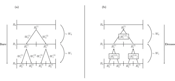
To summarize the above, consider Fig. 1 where a simple downscaling model is de-scribed for a slice through a field. Figure 1a describes the bare cascade, where each rainfall value at a scale levelk is multiplied with two values drawn from the distribution ofWk; in a 2-D setting, 4 values would be drawn. In contrast, Fig. 1b describes the
25
dressing procedure, where each group of rainfall values at scale levelk−1 is averaged to obtain the coarser scale pixel at scale levelk.
HESSD
10, 11385–11422, 2013Imperfect scaling in rainfall
van den Berg et al.
Title Page
Abstract Introduction
Conclusions References
Tables Figures
◭ ◮
◭ ◮
Back Close
Full Screen / Esc
Printer-friendly Version Interactive Discussion
Discussion
P
a
per
|
D
iscussion
P
a
per
|
Discussion
P
a
per
|
Discuss
ion
P
a
per
|
Empirical investigation of the scaling behavior shows that not all rainfall fields obey the basic assumption that the increments between scales are iid. Divergences from this behavior were described by various authors who observed that the increments were dependent on factors such as large scale rainfall intensity (Deidda, 2000; Over and Gupta, 1994) and pixel size (Menabde et al., 1997; Over and Gupta, 1994; Paulson and
5
Baxter, 2007). These deviations from perfect scaling are further examined in Veneziano et al. (2006); Serinaldi (2010), and Rupp et al. (2009), who showed that it is possible to model these imperfections in scaling through empirical functions of the parameters of various downscaling models.
The distributions involved in the above model are often assumed to belong to the
10
family of α-stable distributions (Nolan, 2012), such that their logarithm is distributed as ln(Rk)∼Sα(−1,γ,δ). The α-stable distributionSα is said to be maximally skewed (Rupp et al., 2009), such that its positive moments do exist, or converge to a finite value, allowing for tractable analysis. Despite the obvious relationship between the downscaling model in Eq. (1) and these distributions, no suitable methods exist to
15
reveal which distributions go with which cascades. Although no specific reason for this is known, this can be partly attributed to the fact that the moments in log-space do not uniquely relate to the moments in the untransformed space:E[log(R)q]≤E[log(R)]qfor some momentq, evidently complicating the problem. Moreover,α-stable distributions have no closed form for their Cumulative Distribution Function (CDF) nor does it admit
20
definitive forms of multivariate distributions, resulting in complicated analyses being required to obtain tractable results. Because of this, empirical models are used to relate the distributions to the downscaling model, e.g. see Rupp et al. (2009); Menabde et al. (1999).
In this paper, we wish to develop a model that directly estimates the distributions at
25
various scales of the rainfall field. To do this, we have to approximate the distribution of ln(W), which may be dependent on scale. Moreover, there may be dependencies between the scale levels, which have to be taken into account. Hence, the following questions need to be investigated
HESSD
10, 11385–11422, 2013Imperfect scaling in rainfall
van den Berg et al.
Title Page
Abstract Introduction
Conclusions References
Tables Figures
◭ ◮
◭ ◮
Back Close
Full Screen / Esc
Printer-friendly Version Interactive Discussion
Discussion
P
a
per
|
D
iscussion
P
a
per
|
Discussion
P
a
per
|
Discuss
ion
P
a
per
|
– Is the distribution of ln(Wk) the same for allk?
– Is there dependence between the rainfall field ln(Rk) and its increment ln(Wk)?
– Can we characterize the scaling behavior with a suitable set of equations such that it works for a large number of storms?
Additional to these question, it is interesting to know how well the model works for
5
different rainfall fields. Moreover, characterizing the rainfall field as a set of functions allows us to gain some insight in the behavior of the distribution. As such, the following additional questions will be answered:
– Do the same functions provide an equal fit for all rainfall fields?
– How does the scaling behavior change through time?
10
This paper is structured as follows: in Sect. 2 the data are described, and transfor-mations and operations on the data are explained and motivated. Section 3 presents a basic, preliminary, scaling analysis. In Sect. 4 the α-stable distribution and some of its basic properties are introduced, together with a suitable error measure. Then, the methodology is described in Sect. 5. Subsequently, the results are presented and
15
discussed in Sect. 6. Finally, some conclusions and directions for future research are presented in Sect. 7.
2 Data
The data for this study were acquired by a C-band weather radar near Wideumont, Belgium, operated by the Belgian Royal Meteorological Institute (RMI). This
installa-20
tion covers a circular area with a radius of 240 km, producing a multi-level scan every five minutes. The region covered includes coastal landscapes to the west, and a low mountain range, the Ardennes, to the east with land cover mostly composed of forests,
HESSD
10, 11385–11422, 2013Imperfect scaling in rainfall
van den Berg et al.
Title Page
Abstract Introduction
Conclusions References
Tables Figures
◭ ◮
◭ ◮
Back Close
Full Screen / Esc
Printer-friendly Version Interactive Discussion
Discussion
P
a
per
|
D
iscussion
P
a
per
|
Discussion
P
a
per
|
Discuss
ion
P
a
per
|
urban development and agriculture. The entire region has a temperate climate and re-ceives about 800 mm of rain annually, almost uniformly distributed throughout the year (De Jongh et al., 2006) and a mean monthly temperature which varies between 18◦C in June and 3◦C in January.
The actual 5 min radar images are taken from large events during 2009, with 9 winter
5
storms and 17 summer storms. These images were extracted from a 6 month time se-ries during which larger storm episodes were selected to ensure sufficient data. These images correspond to the basic 5 min interval images, however, to reduce the data load, we opted to use only the first image of each hour. The images used were not ag-gregated in order to retain the basic spatial scaling behavior as well as to avoid ripple
10
effects (Delobbe et al., 2006) and possible temporal scaling.
The raw radar data are produced by a 5-elevation scan performed every 5 min. Mea-surements are collected up to 240 km with a resolution of 250 m in range and 1◦ in azimuth. A time-domain Doppler filtering is applied for ground clutter removal. An addi-tional treatment, based on a static clutter map, is applied to eliminate residual
perma-15
nent ground clutter (e.g. buildings). The radar data are then stored as digital numbers representing the reflectivity values ranging from−31.5 dB to 95.5 dB in steps of 0.5 dB. A two-dimensional radar product is then extracted from the three-dimensional polar data on a Cartesian grid with a resolution of 0.6 km×0.6 km (Goudenhoofdt and De-lobbe, 2009). Reflectivity values are then converted into precipitation rates using
20
R0=
b
s
100.1·ZdB
a , (3)
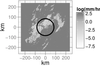
whereZdBis the reflectivity in [dB] andaandbare dimensionless parameters, respec-tively equal to 200 and 1.6. Finally, only the inner 100 km are used in the analysis, as the radar does not produce reliable quantitative estimates outside this range. A sample data image is shown in Fig. 2, where the black circle denotes the 100 km range. Small
25
deviations from this circle are allowed to accommodate the square, aggregated pixels. Additionally, if the image contains less than 10 % active pixels, the image is discarded.
HESSD
10, 11385–11422, 2013Imperfect scaling in rainfall
van den Berg et al.
Title Page
Abstract Introduction
Conclusions References
Tables Figures
◭ ◮
◭ ◮
Back Close
Full Screen / Esc
Printer-friendly Version Interactive Discussion
Discussion
P
a
per
|
D
iscussion
P
a
per
|
Discussion
P
a
per
|
Discuss
ion
P
a
per
|
The processed data were artificially downgraded to obtain a scale cascade of each rainfall image with scales ranging from a pixel size of 0.6 km×0.6 km to 9.6 km×9.6 km, with factorslk=2K−k·0.6 km wherek =0...4. These degraded pixels are obtained by spatially averaging the rainfall depths over squares of the appropriate size (Ferraris et al., 2003a; Deidda, 2000). Thus, the relation between the fine scale fieldRk and the
5
coarse scale fieldR0, can be expressed through Eq. (2). Generally, the scale of the pixels is expressed as
λk =
lk Leff
, (4)
whereLeffis the effective outer scale at which the moments converge. This is an a-priori unknown quantity, which has to be estimated from the data (Lovejoy et al., 2008).
10
3 Scaling analysis
A first step in the analysis of scaling behavior is to establish whether or not the rainfall field is actually scaling, and whether this scaling is multifractal. To provide some insight into this, a single image was analyzed, shown in Fig. 2. For this analysis the field was made conservative by transforming it as (Lovejoy et al., 2008)
15
Rλcons
K =
|∇2(RλK)|
h|∇2(R λK)|i
, (5)
where∇2is the 2-D laplacian, andh·idenotes the average of the field.
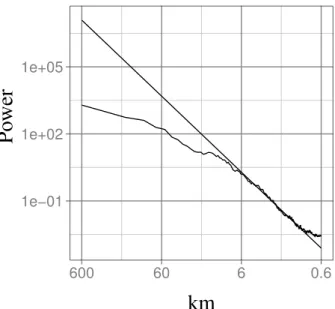
A first tool to assess the scaling behavior is the radially averaged power spectrum, shown in Fig. 3. This figure analyses the full image, without any cutoffs or modifications. In this image, the expectation is to find a linear slope, indicating scaling behavior. Such
20
behavior is observed, as indicated by the linear fit, although a small deviation exists
HESSD
10, 11385–11422, 2013Imperfect scaling in rainfall
van den Berg et al.
Title Page
Abstract Introduction
Conclusions References
Tables Figures
◭ ◮
◭ ◮
Back Close
Full Screen / Esc
Printer-friendly Version Interactive Discussion
Discussion
P
a
per
|
D
iscussion
P
a
per
|
Discussion
P
a
per
|
Discuss
ion
P
a
per
|
at lower scales. This break is likely due to the threshold of the rainfall field as a result of the radar not being able to accurately measure rainfall intensities below 0.1 mm h−1 (Lovejoy et al., 2008).
A basic principle of multifractal behavior is that the (empirical) moments scale as
hRqki
hRq0i =
l
k Lref
K(q)
, (6)
5
whereRk is the rainfall field at scalel=2 (K−k)
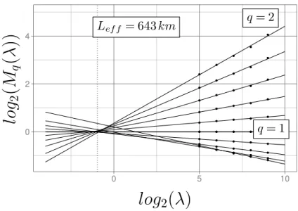
·0.6.Lref is a conveniently chosen outer scale, in lieu of knowing the effective outer scale, and K(q) is the moment scaling function. This function illustrates that if the field is multifractal, the various empirical estimates of a moment q should lie on a straight line in a log-log plot of hRqki/hR0qi
against the scaleλk. By plotting these lines for a variety of moments, shown in Fig. 4,
10
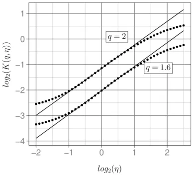
the linearity, and thus multifractal scaling behavior, of each moment can be assessed. As can be seen, these lines are close to linear, further suggesting fractal behavior. The outer scale is the point at which all lines intersect (Lovejoy et al., 2008). This analysis is shown in Fig. 4, for the conservative field, and all moments appear to be appropriately scaling (i.e. linear), which is further confirmed by a Double Trace Moment analysis
15
(Veneziano et al., 2006) shown in Fig. 5. The intersection pointLeff can be difficult to find, as small deviations from linear behavior may prevent the lines from converging. This is solved by forcing the regression lines to convergence at a point for which the RMSE is minimal. Based on this, the effective outer scale for this particular image was found to be about 643 km for this particular storm. However, we should note that such
20
an analysis can be inaccurate, and should only be used as a reference.
4 α-stable distributions
As mentioned in the introduction, the logarithm of the rainfall fieldsRk and their incre-mentsWk are assumed to be distributed according to the α-stable distribution. The
HESSD
10, 11385–11422, 2013Imperfect scaling in rainfall
van den Berg et al.
Title Page
Abstract Introduction
Conclusions References
Tables Figures
◭ ◮
◭ ◮
Back Close
Full Screen / Esc
Printer-friendly Version Interactive Discussion
Discussion
P
a
per
|
D
iscussion
P
a
per
|
Discussion
P
a
per
|
Discuss
ion
P
a
per
|
α-stable family of distributions allows for a large variety in behavior, including right-and left-skewed behavior, as well as symmetric behavior. Furthermore, the distribution allows either a heavy tail or a light, vanishing, tail on either side, or on both sides, of the mode. Due to this highly flexible behavior, it includes several well-known dis-tributions such as the Normal distribution and the Cauchy distribution. The α-stable
5
distribution does not have a closed form, but rather expresses its density as an integral of the characteristic (moment-generating) function over all moments ranging from−∞ to+∞. This would result in an indefinite integral that only has a closed form in a few special cases. Hence, an approximation is required. Although various different approx-imations exist, they are all roughly equivalent and here we used that of Nolan (1997),
10
as implemented in the R-packagestabledistWuertz et al. (2012).
There are a number of different parametrizations available for theα-stable distribu-tion, all suitable for different purposes; we opted for the S1 parametrization of Nolan (2012). Given this parametrization, differentα-stable distributions with (necessarily) the same stability parameterαs, which mainly determines the heaviness of the tail, can be
15
summed as
αZs =αsX =αYs =αs, (7)
βZ =
βXγ
αs X +βYγ
αs Y
γXαs+γYαs , (8)
γZαs=γαXs+γαYs, (9)
δZ =δX+δY. (10)
20
Hereαs∈(0, 2] is a stability parameter, or volatility index, which is necessarily the same for all distributions involved in the above summation. The parameterβrepresents the skewness and ranges from−1 to 1, where 0 represents symmetry,γ >0 is the shape parameter and the shift parameter−∞ ≤δ≤ ∞controls the location of the distribution.
25
Whenαs=2, theα-stable distribution becomes the normal distribution. As a result, the effect of the parameterβ diminishes asαs→2 and has no effect whenαs=2 as
HESSD
10, 11385–11422, 2013Imperfect scaling in rainfall
van den Berg et al.
Title Page
Abstract Introduction
Conclusions References
Tables Figures
◭ ◮
◭ ◮
Back Close
Full Screen / Esc
Printer-friendly Version Interactive Discussion
Discussion
P
a
per
|
D
iscussion
P
a
per
|
Discussion
P
a
per
|
Discuss
ion
P
a
per
|
the normal distribution is necessarily symmetric. Additionally, when αs=2, the shift parameter δ is equal to the mean, and the shape parameter relates to the variance asσ2=√γ/2. Additionally, the distribution only has moments that are smaller thanαs, hence, ifαs≥1 the shift parameter is equal to the mean. Moreover, whenβ=−1, the distribution is entirely left-skewed, meaning that it only has a “fat” tail towards the left.
5
Consequentially, the positive moments converge, whereas the negative moments do not. Fortunately, as we generally only deal with positive moments in rainfall analysis, this property allows for an easy analysis.
Theα-stable distribution can be fitted in a variety of ways, including the well-known Maximum Likelihood method. Nevertheless, fittingα-stable distributions is still a difficult
10
exercise, partly due to the lack of a closed form. Despite these difficulties, numerous different approaches are available and a summary of these approaches can be found in Nolan (1999). For this study, the method of Koutrouvelis (1980) is used together with that of McCulloch (1986). Although an in depth explanation is not within the scope of this paper, the method of McCulloch (1986) relies on a look up table of quantile values
15
and associated parameter values, which is interpolated to obtain a crude first guess estimate of the parameters for the second step. The second step, that of Koutrouvelis (1980), relies on an iterative regression on the characteristic function, together with its empirical counterpart. Essentially, the parameters are updated stepwise by regressing them against the empirical characteristic functionE[exp(√−1qX)] for momentq.
20
Although the above methods produce accurate results in a fast and convenient man-ner, it was observed that the actual results tend to be biased, often as a result of truncated tails in the data. This was mitigated by two procedures. First, several pa-rameters were fixed a priori, namely β=−1 and δ=E[X] where the latter obviously relies onα≥1. Evidently, fixingβ=−1 ensures that the positive moments converge,
25
and the second assumptionδ=E[X] ensures that the averages between the fitted and the empirical probability distributions match. Moreover, the resulting fits were further optimized using a local simplex search to find the optimal parameter set. The resultant parameters provided a better fit than the raw output from the basic fitting algorithm.
HESSD
10, 11385–11422, 2013Imperfect scaling in rainfall
van den Berg et al.
Title Page
Abstract Introduction
Conclusions References
Tables Figures
◭ ◮
◭ ◮
Back Close
Full Screen / Esc
Printer-friendly Version Interactive Discussion
Discussion
P
a
per
|
D
iscussion
P
a
per
|
Discussion
P
a
per
|
Discuss
ion
P
a
per
|
Finally, to quantify the quality of the fit, the Earth Movers Distance (EMD) is used. The EMD is a measure similar to other error measures such as the Root Mean Squared Error and the Mean Absolute Error (van den Berg et al., 2011; Rubner and Tomasi, 1999), however, it accounts for both vertical and horizontal differences between prob-ability distribution functions such that, for example, shifts in mean are appropriately
5
taken into account. This difference between RMSE and EMD becomes important when the distribution has a strong peak, such as exponential-like distributions. As these can be encountered in the subset of the α-stable distribution, this metric shows a more stable performance than does the RMSE.
5 Methodology 10
The starting point for any analysis is the rainfall intensity field R0. In this study, the resolution of these images is degraded to find a synthetic cascade, using Eq. (2). The result is a set of rainfall imagesRk withk ∈(0..K) with increasing (coarsening) scale. By taking the log-transform of these fields, the log-increments ln(Wk),k∈(0..K−1) can be extracted as
15
ln(Wk)=ln(Rk+1)−ln(Rk+1)=ln
R
k Rk+1
, (11)
where the difference in the number of pixels is overcome by repeating the action for each pixel and its coarse scale pixel. The resulting cascades can then be analyzed by fitting anα-stable distribution to each of the fields ln(Wk) and ln(Rk) for k∈(0..K). Moreover, as mentioned earlier, the parameter αs should be the same for all these
20
distributions. Therefore, the fit is done in two steps, first a preliminary step where all distributions are fitted separately resulting in a setαis=0..K, which contains all valuesαs
for both the increments and the fields. Then, the distributions are fitted a second time, forcingαs=hαis=0..Ki. Although no formal relationship exists between distributions with differentαs, it was found that the mean of a set was in good agreement with optimized
25
HESSD
10, 11385–11422, 2013Imperfect scaling in rainfall
van den Berg et al.
Title Page
Abstract Introduction
Conclusions References
Tables Figures
◭ ◮
◭ ◮
Back Close
Full Screen / Esc
Printer-friendly Version Interactive Discussion
Discussion
P
a
per
|
D
iscussion
P
a
per
|
Discussion
P
a
per
|
Discuss
ion
P
a
per
|
values ofαs. Hence, this analysis results in a set of parameters (αsW,−1,γWk,δWk) for each scale levelk, where it should be noted thatδW
k is forced to be equal tohln(Wk)i. A similar set is found for each rainfall field ln(Rk), denoted by subscriptRk.
Besides the basic parameters of the distribution, we are also interested in establish-ing whether or not the fields and their increments are actually iid. A simple test would
5
be to use the correlation to assess whether or not these distributions are uncorrelated. However, theα-stable distribution with stability parameterαsdoes not admit moments
q> αs, hence, ifαs<2 the (Pearson) correlation does not exist. As a result, using raw
correlations is not feasible, and a difficult problem in α-stable analysis arises. Many different measures have been suggested, but to the authors’ knowledge all of these
10
pertain to symmetric distributions, i.e. those with β=0. Nonetheless, we adopt the correlation value of Garel and Kodia (2009) as it offers important benefits and presents a conceptually simple framework.
The basis of the correlation value of Garel and Kodia (2009) relies on the notion that, for properly scaled variables with finite second order moments, the slope of the
re-15
gressionE[R|W]=E[W|R] (note that the logarithm and the scale indicators have been dropped for notational convenience) is equal to the Pearson correlationρ. However, the regression line and its slope always exist, in contrast to the Pearson correlation coefficient, even though we cannot generally say that it is finite or exchangeable (i.e. it could be thatE[R|W]6=E[W|R]). Hence, an appealing correlation measure is
20
̺(R,W)=sign(θR|W)
q
θR|WθW|R, (12)
whereθR|W is the slope of the regression lineE[R|W], and similarly forθW|R. Use of the square root is to ensure that if the second order moment exists, the metric coincides with the Pearson correlation. Finally, the sign function is used to ensure that negative and positive correlations are differentiated. A proof for this metric is beyond scope of
25
the paper, rather, we will investigate its practical skill.
The relationship between the shape parameters of the rainfall field and its incre-ments,γW and γR, with̺(R,W)6=0 is dependent on the entire bivariate distribution
HESSD
10, 11385–11422, 2013Imperfect scaling in rainfall
van den Berg et al.
Title Page
Abstract Introduction
Conclusions References
Tables Figures
◭ ◮
◭ ◮
Back Close
Full Screen / Esc
Printer-friendly Version Interactive Discussion
Discussion
P
a
per
|
D
iscussion
P
a
per
|
Discussion
P
a
per
|
Discuss
ion
P
a
per
|
(Nolan, 2012). However, modeling such a distribution is highly cumbersome and not at all evident as multivariate stable distributions are an area of ongoing research; There-fore, a simplification is needed. We observe that ifαs=2 the relationship betweenγW andγRis
γRαs+W =γRαs+γαS
W +ρ(2σ αs R )
(1/αs)(2σαs W)
(1/αs), (13)
5
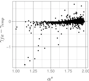
whereρ denotes the Pearson correlation coefficient. The above is dependent on the notion that ifαs=2 theα-stable distribution becomes a normal distribution, with vari-ance 2γαs. Therefore, to simulate the effects of the summation of a correlated distribu-tion, we use Eq. (13) where we substituteρ with̺. The effects of using this equation are investigated in Fig. 6 by comparing shape parameters fitted to the empirical
distri-10
bution with shape parameters computed according to Eq. (13). Note that, in general, the errors appear to be mild, however, at lower values ofαs, several large errors can be observed. Fortunately, few rainfall images have distributions with lowαs, making this a tenable assumption.
To investigate the behavior of the scaling of theα-stable parameters through time,
15
we first need to characterize this behavior for each of the images. This is done by fitting a set of scale dependent functions to theα-stable parameters for each image and its increments. The mean behavior of theα-stable parameters for all images was used as a guideline for the function forms, shown in Figs. 7 to 9. These empirical functions all admit relatively simple function forms, namely
20
δk =aδ+bδ·ln(λ) , (14)
γk=eaγ+bγ·ln(λ), (15)
̺k=a̺+b̺·
1
λ. (16)
Note that the subscripts identifying that these parameters apply to ln(Wk) have been
25
HESSD
10, 11385–11422, 2013Imperfect scaling in rainfall
van den Berg et al.
Title Page
Abstract Introduction
Conclusions References
Tables Figures
◭ ◮
◭ ◮
Back Close
Full Screen / Esc
Printer-friendly Version Interactive Discussion
Discussion
P
a
per
|
D
iscussion
P
a
per
|
Discussion
P
a
per
|
Discuss
ion
P
a
per
|
the range is [0,∞[. The equation for ̺ is not bounded as the correlation measure used is not. The fit of the above functions is examined in Figs. 7 to 9, for each of the parameters respectively. The confidence intervals of each of the functions are relatively small, and the behavior is well respected. Nevertheless, the function forδk appears to have a slight curve to it, possibly suggesting a more complex behavior. However, due
5
to the limited number of scale levels available fitting a more complex function was not feasible.
To summarize the above, we retake Fig. 1, specifically the distribution W0∼ Sα(−1,γ0,µ0) and the same distribution at further scales. The valuesγk andδk at all scales are found through Eqs. (14) to (16). Then, having the distribution of the coarsest
10
scale rainfall, ln(R0), we can findR1using̺0applying Eq. (13) withρsubstituted with
̺. Applying this framework iteratively, it is possible to findR2and so on.
Finally, the number of dry pixels are modeled based on the fractal box counting dimension (Rupp et al., 2009). As the boxcounting dimension is directly based on the number of dry pixels at each scale, it suffices to invert this relationship
15
P(Y >0)l=
1
lk
Df
·P(Y>0)l
k=1 (17)
whereDf is the fractal dimension and lk is the side length of the pixel at scale k ex-pressed in elementary pixels. This relationship performs near perfect (Fig. 10).
6 Scaling behavior
In Fig. 11 all the correlations for each of the scales are shown, summarized as a
box-20
plot. From this plot, it is evident that almost all storms exhibit a negative correlation be-tween the increments and the rainfall field. This pattern is also seen in rank correlation measures (not shown), further corroborating that there is indeed negative correlation. Taking this negative correlation into account according to Eq. (13) indeed results in a decrease in error, as is evidenced by the lower EMD for the correlated than for the
25
HESSD
10, 11385–11422, 2013Imperfect scaling in rainfall
van den Berg et al.
Title Page
Abstract Introduction
Conclusions References
Tables Figures
◭ ◮
◭ ◮
Back Close
Full Screen / Esc
Printer-friendly Version Interactive Discussion
Discussion
P
a
per
|
D
iscussion
P
a
per
|
Discussion
P
a
per
|
Discuss
ion
P
a
per
|
uncorrelated error (Fig. 12). Moreover, the significant decrease in the shape parameter,
γfurther suggest that the iid assumption is, for these storms, incorrect.
The functions (14) to (16) are used to characterize the scaling behavior. These func-tions exhibit a good fit for all storms, as determined through the relative error (Fig. 13). The resulting parameters are shown for each storm in Figs. 14 to 16. From these
box-5
plots, it can be seen that summer storms exhibit a higher spread of all parameter values and a higher mean of the increments. However, the̺shows no difference in intercept, but the decrease in̺ for winter storms is higher than for summer storms. However, there is no real clear pattern distinguishing the behavior between the winter and sum-mer storms.
10
The analyses confirm the common finding summer that storms tend to be more energetic with higher variances and higher mean rainfall. Moreover, summer storms appear to exhibit a smaller decrease in correlations, resulting in a stronger correlation at the lower scale levels.
Figure 17 shows the difference between the EMDs of the modeled distributions and
15
the direct fitted distributions, propagated over the four scale levels. It can be seen that the model increases the EMD as the number of scale levels increases. Nonetheless, the error remains relatively low, showing that the model captures the scaling behavior quite well. The fractal model for the dry pixels works very well, as should be expected due to the direct relation with the actual number of dry pixels.
20
7 Conclusions
In this paper, we investigated the scaling behavior of the distributions of rainfall. To this end, a novel scaling model was introduced that only relies on the basic assumptions re-garding the cascade structure responsible for the fractal nature of rainfall. Furthermore, this framework is based on direct empirical comparison with the observed distributions.
25
In contrast, most previous work relied on theoretical considerations and indirect use of the scaling distributions. Therefore, this framework allows for a more direct and
HESSD
10, 11385–11422, 2013Imperfect scaling in rainfall
van den Berg et al.
Title Page
Abstract Introduction
Conclusions References
Tables Figures
◭ ◮
◭ ◮
Back Close
Full Screen / Esc
Printer-friendly Version Interactive Discussion
Discussion
P
a
per
|
D
iscussion
P
a
per
|
Discussion
P
a
per
|
Discuss
ion
P
a
per
|
ical investigation into the scaling behavior of rainfall, and provides a more adaptable framework to be used for practical purposes.
The empirical investigation into the distribution showed that the shape parameter, loosely related to the variance, of finer scales is smaller than its parent scale. This contradicts the classical scaling theory (Lovejoy and Mandelbrot, 1985) that
uncorre-5
lated increment distributions are added, as this would cause an increase in the shape parameter. Moreover, it was shown that it is possible to improve these predictions by taking into account the correlation. Although the method used to add the correlations is only correct whenαs=2, using an approximate equation improved performance. This suggests that there is, in fact, imperfect scaling in all of the investigated images.
10
In this paper, imperfect scaling behavior was characterized using three simple equa-tions (Eqs. 14 to 16). It was found that these equaequa-tions fit well, and are successful in describing the general behavior of the distribution for all observed images.
In future research, the full dependence structure will need to be evaluated to allow for a more accurate representation of the dependence between scale levels and their
15
increments. This will allow for a deeper investigation into this aspect of imperfect scaling and possible a better way of representing the scaling behavior. Finally, the difference with respect to the scaling behavior, between convective and stratiform storms will need further investigation, using a classification algorithm such as the Steiner algorithm (Steiner et al., 1995). A careful analysis of the behavior of such algorithms will be
20
required before using them to investigate the difference in scaling behaviour between stratiform and convective precipitation.
Acknowledgements. We wish to thank the Special Research Fund (B.O.F.) of Ghent University and the Flanders Research Fund (FWO, Grant Number: G.0837.10) for funding this research.
HESSD
10, 11385–11422, 2013Imperfect scaling in rainfall
van den Berg et al.
Title Page
Abstract Introduction
Conclusions References
Tables Figures
◭ ◮
◭ ◮
Back Close
Full Screen / Esc
Printer-friendly Version Interactive Discussion
Discussion
P
a
per
|
D
iscussion
P
a
per
|
Discussion
P
a
per
|
Discuss
ion
P
a
per
|
References
Bergström, S., Carlsson, B., Gardelin, M., Lindstrom, G., Pettersson, A., and Rummukainen, M.: Climate change impacts on runoffin Sweden – assessments by global climate models, dy-namical downscaling and hydrological modelling, Clim. Res., 16, 101–112, 2001. 11386 Castelli, F.: Atmosphere modeling and hydrologic-prediction uncertainty, invited lecture at the 5
US-Italy Workshop on the Hydrometeorology, Impacts and Management of Extreme Floods, Perugia, Abstract 2.2, 13–17 November, 1995. 11386
De Jongh, I. L. M., Verhoest, N. E. C., and De Troch, F. P.: Analysis of a 105-year time series of precipitation observed at Uccle, Belgium, Int. J. Climatol., 26, 2023–2039, 2006. 11391 Deidda, R.: Rainfall downscaling in a space-time multifractal framework, Water Resour. Res., 10
36, 1779–1794, 2000. 11387, 11389, 11392
Delobbe, L., Dehem, D., Dierickx, P., Roulin, E., Thunus, M., and Tricot, C.: Combined use of radar and gauge observations for hydrological applications in the Walloon region of Belgium, in: Proceedings of ERAD, Barcelona, 418–421, 2006. 11391
Dibike, Y. B. and Coulibaly, P.: Hydrologic impact of climate change in the Saguenay watershed: 15
comparison of downscaling methods and hydrologic models, J. Hydrol., 307, 145–163, 2005. 11386
Ferraris, L., Rudari, R., and Siccardi, F.: The uncertainty in the prediction of flash floods in the northern Mediterranean environment, J. Hydrometeorol., 3, 714–727, 2002. 11386, 11388 Ferraris, L., Gabellani, S., Parodi, U., Rebora, N., Von Hardenberg, J., and Provenzale, A.: 20
Revisiting multifractality in rainfall fields, J. Hydrometeorol., 4, 544–551, 2003a. 11392 Ferraris, L., Gabellani, S., Rebora, N., and Provenzale, A.: A comparison of stochastic models
for spatial rainfall downscaling, Water Resour. Res., 39, 1368, doi:10.1029/2003WR002504, 2003b. 11386
Garel, B. and Kodia, B.: Signed symmetric covariation coefficient for alpha-stable dependence 25
modeling, CR Math., 347, 315–320, 2009. 11397
Goudenhoofdt, E. and Delobbe, L.: Evaluation of radar-gauge merging methods for quantita-tive precipitation estimates, Hydrol. Earth Syst. Sci., 13, 195–203, doi:10.5194/hess-13-195-2009, 2009. 11391
Gupta, V. K. and Waymire, E. C.: A statistical analysis of mesoscale rainfall as a random cas-30
cade, J. Appl. Meteorol., 32, 251–251, 1993. 11387
HESSD
10, 11385–11422, 2013Imperfect scaling in rainfall
van den Berg et al.
Title Page
Abstract Introduction
Conclusions References
Tables Figures
◭ ◮
◭ ◮
Back Close
Full Screen / Esc
Printer-friendly Version Interactive Discussion
Discussion
P
a
per
|
D
iscussion
P
a
per
|
Discussion
P
a
per
|
Discuss
ion
P
a
per
|
Koutrouvelis, I.: Regression-type estimation of the parameters of stable laws, J. Am. Stat. As-soc., 75, 918–928, 1980. 11395
Koutsoyiannis, D., Paschalis, A., and Theodoratos, N.: Two-dimensional Hurst–Kolmogorov pro-cess and its application to rainfall fields, J. Hydrol., 398, 91–100, 2010. 11387
Lilley, M., Lovejoy, S., Desaulniers-Soucy, N., and Schertzer, D.: Multifractal large number of 5
drops limit in rain, J. Hydrol., 328, 20–37, 2006. 11387
Lovejoy, S. and Mandelbrot, B. B.: Fractal properties of rain, and a fractal model, Tellus A, 37, 209–232, 1985. 11387, 11388, 11401
Lovejoy, S. and Schertzer, D.: Fractals, raindrops and resolution dependence of rain measure-ments, J. Appl. Meteorol., 29, 1167–1170, 1990. 11387
10
Lovejoy, S. and Schertzer, D.: Multifractals, cloud radiances and rain, J. Hydrol., 322, 59–88, 2006. 11387
Lovejoy, S. and Schertzer, D.: On the simulation of continuous in scale universal multifractals, Part I: Spatially continuous processes, Comput. Geosci., 36, 1393–1403, 2010a. 11387 Lovejoy, S. and Schertzer, D.: On the simulation of continuous in scale universal multifractals, 15
Part II: Space-time processes and finite size corrections, Comput. Geosci., 36, 1404–1413, 2010b. 11387
Lovejoy, S., Schertzer, D., and Stanway, J. D.: Direct evidence of multifractal atmospheric cas-cades from planetary scales down to 1 km, Phys. Rev. Lett., 86, 5200–5203, 2001. 11387 Lovejoy, S., Schertzer, D., and Allaire, V. C.: The remarkable wide range spatial scaling of 20
TRMM precipitation, Atmos. Res., 90, 10–32, 2008. 11387, 11392, 11393
McCulloch, J.: Simple consistent estimators of stable distribution parameters, Commun. Stat. Simulat., 15, 1109–1136, 1986. 11395
Menabde, M. and Sivapalan, M.: Modeling of rainfall time series and extremes using bounded random cascades and Levy-stable distributions, Water Resour. Res., 36, 3293–3300, 2000. 25
11387
Menabde, M., Harris, D., Seed, A., Austin, G., and Stow, D.: Multiscaling properties of rainfall and bounded random cascades, Water Resour. Res., 33, 2823–2830, 1997. 11387, 11389 Menabde, M., Seed, A., and Pegram, G.: A simple scaling model for extreme rainfall, Water
Resour. Res., 35, 335–339, 1999. 11389 30
Nolan, J. P.: Parameter estimation and data analysis for stable distributions, in: Conference Record of the Thirty-First Asilomar Conference on Signals, Systems & Computers, 1997, vol. 1, IEEE, Pacific Grove(CA), USA, 443–447, 1997. 11394
HESSD
10, 11385–11422, 2013Imperfect scaling in rainfall
van den Berg et al.
Title Page
Abstract Introduction
Conclusions References
Tables Figures
◭ ◮
◭ ◮
Back Close
Full Screen / Esc
Printer-friendly Version Interactive Discussion
Discussion
P
a
per
|
D
iscussion
P
a
per
|
Discussion
P
a
per
|
Discuss
ion
P
a
per
|
Nolan, J. P.: Fitting data and assessing goodness-of-fit with stable distributions, unpublished manuscript, American University, Washington, DC, 1999. 11395
Nolan, J. P.: Stable Distributions – Models for Heavy Tailed Data, Birkhauser, Boston, in progress, Chapter 1 available at: http://academic2.american.edu/~jpnolan (last ac-cess: 20 August 2013), 2012. 11389, 11394, 11398
5
Over, T. and Gupta, V.: Statistical analysis of mesoscale rainfall: dependence of a random cascade generator on large-scale forcing, J. Appl. Meteorol., 33, 1526–1542, 1994. 11389 Paulson, K. S. and Baxter, P. D.: Downscaling of rain gauge time series by multiplicative beta
cascade, J. Geophys. Res., 112, D09105, doi:10.1029/2006JD007333, 2007. 11389 Rahman, S., Bagtzoglou, A. C., Hossain, F., Tang, L., Yarbrough, L. D., and Easson, G.: Inves-10
tigating spatial downscaling of satellite rainfall data for streamflow simulation in a medium-sized basin, J. Hydrometeorol., 10, 1063–1079, 2009. 11386
Rebora, N., Ferraris, L., von Hardenberg, J., and Provenzale, A.: Rainfall downscaling and flood forecasting: a case study in the Mediterranean area, Nat. Hazards Earth Syst. Sci., 6, 611– 619, doi:10.5194/nhess-6-611-2006, 2006. 11386, 11388
15
Rubner, Y. and Tomasi, C.: Texture-based image retrieval without segmentation, in: The Pro-ceedings of the Seventh IEEE International Conference on Computer Vision, 1999, vol. 2, IEEE, Corfu, Greece, 1018–1024, 1999. 11396
Rupp, D. E., Keim, R. F., Ossiander, M., Brugnach, M., and Selker, J. S.: Time scale and in-tensity dependency in multiplicative cascades for temporal rainfall disaggregation, Water Re-20
sour. Res., 45, W07409, doi:10.1029/2008WR007321, 2009. 11388, 11389, 11399
Schertzer, D. and Lovejoy, S.: Physical modeling and analysis of rain and clouds by anisotropic scaling multiplicative processes, J. Geophys. Res., 92, 9693–9714, 1987. 11387
Serinaldi, F.: Multifractality, imperfect scaling and hydrological properties of rainfall time series simulated by continuous universal multifractal and discrete random cascade models, Nonlin-25
ear Proc. Geoph., 17, 697–714, 2010. 11389
Steiner, M., Houze Jr., R. A., and Yuter, S. E.: Climatological characterization of three-dimensional storm structure from operational radar and rain gauge data, J. Appl. Meteorol., 34, 1978–2007, 1995. 11401
van den Berg, M. J., Vandenberghe, S., De Baets, B., and Verhoest, N. E. C.: Copula-based 30
downscaling of spatial rainfall: a proof of concept, Hydrol. Earth Syst. Sci., 15, 1445–1457, doi:10.5194/hess-15-1445-2011, 2011. 11396
HESSD
10, 11385–11422, 2013Imperfect scaling in rainfall
van den Berg et al.
Title Page
Abstract Introduction
Conclusions References
Tables Figures
◭ ◮
◭ ◮
Back Close
Full Screen / Esc
Printer-friendly Version Interactive Discussion
Discussion
P
a
per
|
D
iscussion
P
a
per
|
Discussion
P
a
per
|
Discuss
ion
P
a
per
|
Veneziano, D., Furcolo, P., and Iacobellis, V.: Imperfect scaling of time and space-time rainfall, J. Hydrol., 322, 105–119, 2006. 11389, 11393
Wuertz, D., Maechler, M., and R core team members: stabledist: Stable Distribution Functions, r package version 0.6-5, available at: http://CRAN.R-project.org/package=stabledist, 2012. 11394
5
HESSD
10, 11385–11422, 2013Imperfect scaling in rainfall
van den Berg et al.
Title Page
Abstract Introduction
Conclusions References
Tables Figures
◭ ◮
◭ ◮
Back Close
Full Screen / Esc
Printer-friendly Version Interactive Discussion
Discussion
P
a
per
|
D
iscussion
P
a
per
|
Discussion
P
a
per
|
Discuss
ion
P
a
per
|
P
ap
er
|
Disussion
P
ap
er
|
Disussion
P
ap
er
|
Disussion
P
ap
er
R2
R1
R(1)0
R0
·W0(2)
R(2)1
·W0(1)
R(1)1
·W1(4)
R(4)2
·W1(3)
R2(3)
·W1(1)
R(1)2
·W1(2)
R(2)2
∼W0
∼W1
Bare
(a) (b)
R2
R1
R(1)0
R0
R(2)1
hR(1,2)
1 i
R(1)1
R(3)2 R(4)2
R(2)2
R(1)2
hR(12,2)i hR(32,4)i
∼W0
∼W1
Dressed
Fig. 1. A basic rainfall model, graphically illustrated. The left hand side of the image is the
dressing procedure, whereas the right hand side is the generation.
HESSD
10, 11385–11422, 2013Imperfect scaling in rainfall
van den Berg et al.
Title Page
Abstract Introduction
Conclusions References
Tables Figures
◭ ◮
◭ ◮
Back Close
Full Screen / Esc
Printer-friendly Version Interactive Discussion
Discussion
P
a
per
|
D
iscussion
P
a
per
|
Discussion
P
a
per
|
Discuss
ion
P
a
per
|
P
ap
er
|
Disussion
P
ap
er
|
Disussion
P
ap
er
|
Disussion
P
ap
er
−
200
−
100
0
100
200
−
200
−
100 0
100 200
km
km
−
7.5
−
5.0
−
2.5
0.0
2.5
log(mm/hr)
Fig. 2.A log-transformed rainfall field, together with the radius of reliable observations.
HESSD
10, 11385–11422, 2013Imperfect scaling in rainfall
van den Berg et al.
Title Page
Abstract Introduction
Conclusions References
Tables Figures
◭ ◮
◭ ◮
Back Close
Full Screen / Esc
Printer-friendly Version Interactive Discussion
Discussion
P
a
per
|
D
iscussion
P
a
per
|
Discussion
P
a
per
|
Discuss
ion
P
a
per
|
P
ap
er
|
Disussion
P
ap
er
|
Disussion
P
ap
er
|
Disussion
P
ap
er
|
1e−01 1e+02 1e+05
600 60 6 0.6
km
P
o
w
e
r
Fig. 3.The power spectrum of the field of storm 1 at time 1.
HESSD
10, 11385–11422, 2013Imperfect scaling in rainfall
van den Berg et al.
Title Page
Abstract Introduction
Conclusions References
Tables Figures
◭ ◮
◭ ◮
Back Close
Full Screen / Esc
Printer-friendly Version Interactive Discussion
Discussion
P
a
per
|
D
iscussion
P
a
per
|
Discussion
P
a
per
|
Discuss
ion
P
a
per
|
P
ap
er
|
Disussion
P
ap
er
|
Disussion
P
ap
er
|
Disussion
P
ap
er
0 2 4
0 5 10
log
2(
λ
)
lo
g
2(
M
q
(
λ
))
q= 1
q= 2
Lef f = 643km
Fig. 4.The empirical momentsMqas a function of scale.
HESSD
10, 11385–11422, 2013Imperfect scaling in rainfall
van den Berg et al.
Title Page
Abstract Introduction
Conclusions References
Tables Figures
◭ ◮
◭ ◮
Back Close
Full Screen / Esc
Printer-friendly Version Interactive Discussion
Discussion
P
a
per
|
D
iscussion
P
a
per
|
Discussion
P
a
per
|
Discuss
ion
P
a
per
|
Disussion
P
ap
er
|
Disussion
P
ap
er
|
Disussion
P
ap
er
|
Disussion
P
ap
er
|
−4 −3 −2 −1 0 1
−2 −1 0 1 2
log2(η)
lo
g2
(
K
(
q
,η
))
q= 2
q= 1.6
Fig. 5.The double trace moments of the field of storm 1 at time 1.
HESSD
10, 11385–11422, 2013Imperfect scaling in rainfall
van den Berg et al.
Title Page
Abstract Introduction
Conclusions References
Tables Figures
◭ ◮
◭ ◮
Back Close
Full Screen / Esc
Printer-friendly Version Interactive Discussion
Discussion
P
a
per
|
D
iscussion
P
a
per
|
Discussion
P
a
per
|
Discuss
ion
P
a
per
|
P
ap
er
|
Disussion
P
ap
er
|
Disussion
P
ap
er
|
Disussion
P
ap
er
|
−1 0
1.00 1.25 1.50 1.75 2.00
α
sγ
fit
−
γ
emp
Fig. 6.The difference between the parameterγ at the second coarsest scale, fitted and
empir-ically fitted.
HESSD
10, 11385–11422, 2013Imperfect scaling in rainfall
van den Berg et al.
Title Page
Abstract Introduction
Conclusions References
Tables Figures
◭ ◮
◭ ◮
Back Close
Full Screen / Esc
Printer-friendly Version Interactive Discussion
Discussion
P
a
per
|
D
iscussion
P
a
per
|
Discussion
P
a
per
|
Discuss
ion
P
a
per
|
0.0 0.1 0.2
2.5 5.0 7.5
2k
∗0.6 (km)
δk
Fig. 7.The empirical means of the increments, averaged over all images, and its fit.
HESSD
10, 11385–11422, 2013Imperfect scaling in rainfall
van den Berg et al.
Title Page
Abstract Introduction
Conclusions References
Tables Figures
◭ ◮
◭ ◮
Back Close
Full Screen / Esc
Printer-friendly Version Interactive Discussion
Discussion
P
a
per
|
D
iscussion
P
a
per
|
Discussion
P
a
per
|
Discuss
ion
P
a
per
|
P
ap
er
|
Disussion
P
ap
er
|
Disussion
P
ap
er
|
Disussion
P
ap
er
|
−0.1 0.0 0.1 0.2 0.3 0.4
2.5 5.0 7.5
2
k∗
0
.
6
(km)
γ
kFig. 8.The empirically fittedγ of the increments, averaged over all images, and its fit.
HESSD
10, 11385–11422, 2013Imperfect scaling in rainfall
van den Berg et al.
Title Page
Abstract Introduction
Conclusions References
Tables Figures
◭ ◮
◭ ◮
Back Close
Full Screen / Esc
Printer-friendly Version Interactive Discussion
Discussion
P
a
per
|
D
iscussion
P
a
per
|
Discussion
P
a
per
|
Discuss
ion
P
a
per
|
P
ap
er
|
Disussion
P
ap
er
|
Disussion
P
ap
er
|
Disussion
P
ap
er
|
−0.4 −0.3 −0.2
2.5 5.0 7.5
2
k∗
0
.
6
(km)
̺
kFig. 9.The empirical̺of the increments, averaged over all images, and its fit.
HESSD
10, 11385–11422, 2013Imperfect scaling in rainfall
van den Berg et al.
Title Page
Abstract Introduction
Conclusions References
Tables Figures
◭ ◮
◭ ◮
Back Close
Full Screen / Esc
Printer-friendly Version Interactive Discussion
Discussion
P
a
per
|
D
iscussion
P
a
per
|
Discussion
P
a
per
|
Discuss
ion
P
a
per
|
P
ap
er
|
Disussion
P
ap
er
|
Disussion
P
ap
er
|
Disussion
P
ap
er
|
0.0 0.1 0.2
0.6 1.2 2.4 4.8 9.6
P
(
R
k=
0)
2
k∗
0
.
6
(km)
Fig. 10.The difference between the probability of dry pixels as predicted, and as observed.
HESSD
10, 11385–11422, 2013Imperfect scaling in rainfall
van den Berg et al.
Title Page
Abstract Introduction
Conclusions References
Tables Figures
◭ ◮
◭ ◮
Back Close
Full Screen / Esc
Printer-friendly Version Interactive Discussion
Discussion
P
a
per
|
D
iscussion
P
a
per
|
Discussion
P
a
per
|
Discuss
ion
P
a
per
|
Disussion
P
ap
er
|
Disussion
P
ap
er
|
Disussion
P
ap
er
|
Disussion
P
ap
er
|
−0.6 −0.4 −0.2 0.0
1 2 3 4 5 6 7 8 9 10 11 12 13 14 15 16 17 18 19 20 21 22 23 24 25 26
Storm
winter summer
̺
Fig. 11.The correlations of all scales for each of the storms.
HESSD
10, 11385–11422, 2013Imperfect scaling in rainfall
van den Berg et al.
Title Page
Abstract Introduction
Conclusions References
Tables Figures
◭ ◮
◭ ◮
Back Close
Full Screen / Esc
Printer-friendly Version Interactive Discussion
Discussion
P
a
per
|
D
iscussion
P
a
per
|
Discussion
P
a
per
|
Discuss
ion
P
a
per
|
P
ap
er
|
Disussion
P
ap
er
|
Disussion
P
ap
er
|
Disussion
P
ap
er
|
0.0 0.2 0.4
0.6 1.2 2.4 4.8 9.6
E
M
D
no
co
r
r.
−
E
M
D
cor
r.
2
k∗
0
.
6
(km)
Fig. 12.The difference between the EMD of the distribution without correlation, and that with
correlation.
HESSD
10, 11385–11422, 2013Imperfect scaling in rainfall
van den Berg et al.
Title Page
Abstract Introduction
Conclusions References
Tables Figures
◭ ◮
◭ ◮
Back Close
Full Screen / Esc
Printer-friendly Version Interactive Discussion
Discussion
P
a
per
|
D
iscussion
P
a
per
|
Discussion
P
a
per
|
Discuss
ion
P
a
per
|
−1.0 −0.5 0.0 0.5 1.0
1 2 3 4 5 6 7 8 9 10 11 12 13 14 15 16 17 18 19 20 21 22 23 24 25 26
Storm
winter summer
−0.2 −0.1 0.0 0.1 0.2
1 2 3 4 5 6 7 8 9 10 11 12 13 14 15 16 17 18 19 20 21 22 23 24 25 26
Storm
winter summer
−0.50 −0.25 0.00 0.25 0.50
1 2 3 4 5 6 7 8 9 10 11 12 13 14 15 16 17 18 19 20 21 22 23 24 25 26
Storm
winter summer
δe
m
p
−
δf
i
t
δe
m
p
γe
m
p
−
γf
it
γe
m
p
̺e
m
p
−
̺f
it
̺e
m
p
Fig. 13.The relative errors of the mean, shape and correlation parameters.