www.nonlin-processes-geophys.net/16/579/2009/ © Author(s) 2009. This work is distributed under
the Creative Commons Attribution 3.0 License.
in Geophysics
Multiscaling analysis of high resolution space-time lidar-rainfall
P. V. Mandapaka, P. Lewandowski, W. E. Eichinger, and W. F. Krajewski
IIHR-Hydroscience & Engineering, The University of Iowa, Iowa City, Iowa, USA
Received: 5 April 2009 – Revised: 27 August 2009 – Accepted: 2 September 2009 – Published: 24 September 2009
Abstract. In this study, we report results from scaling anal-ysis of 2.5 m spatial and 1 s temporal resolution lidar-rainfall data. The high resolution spatial and temporal data from the same observing system allows us to investigate the variabil-ity of rainfall at very small scales ranging from few meters to
∼1 km in space and few seconds to∼30 min in time. The re-sults suggest multiscaling behaviour in the lidar-rainfall with the scaling regime extending down to the resolution of the data. The results also indicate the existence of a space-time transformation of the formt∼Lzat very small scales, where
tis the time lag,Lis the spatial averaging scale andzis the dynamic scaling exponent.
1 Introduction
Spatial and temporal variability of rainfall across multi-ple scales is of fundamental interest to meteorologists and hydrologists. In the last two decades, multiscaling-based framework has been increasingly used by researchers to sta-tistically characterize the rainfall variability over a range of temporal and spatial scales (e.g., Schertzer and Lovejoy, 1987; Tessier et al., 1993; Gupta and Waymire, 1993; Geor-gakakos et al., 1994; Veneziano et al., 1996; Venugopal et al., 1999; Lilley et al., 2006; Lovejoy and Schertzer, 2006; Lovejoy et al., 2008). While the temporal scales varied from few seconds to years (e.g., Georgakakos et al., 1994; Ols-son et al., 1993), the spatial scales varied from few hundreds of meters to continental scales (e.g., Lovejoy and Schertzer, 2006; Lovejoy et al., 2008). Although rainfall is comprised of individual rain drops, it is usually studied as a continu-ous field under the assumption of large number (N) of drops. Lilley et al. (2006) showed evidence of multifractal nature of this N-limit in rain based on the data collected during the HYDROP experiment (Desaulniers-Soucy et al., 2001). In
Correspondence to:P. V. Mandapaka ([email protected])
this study we aim to investigate the presence of multiscaling in rainfall at very small scales ranging from few meters to
∼1 km in space and few seconds to∼30 min in time using the 2.5 m and 1 s resolution rainfall data measured by lidar over Iowa City, Iowa, USA (Lewandowski et al., 2009). Our study therefore contributes towards understanding the mul-tiscale statistical properties of rainfall at space-time scales that received little attention, as shown in the following brief review of the literature.
A physical process is said to be scale-invariant or scal-ing, if large scale and small scale structures are related by a scale-changing operation that involves only the scale ratio and an exponent (e.g., Schertzer and Lovejoy, 1987). If dif-ferent exponents are required to describe the scaling behavior of different moments, then the process is said to be multi-scaling. Studies have shown that multiscaling behaviour is a result of multiplicative cascades, where large scale struc-tures feed small scale strucstruc-tures (e.g., Schertzer and Lovejoy, 1987; Lovejoy et al., 1990). This results in higher and higher intensities being concentrated into smaller and smaller areas, which is true of rainfall process. In addition to understand-ing rainfall processes across multiple scales, other attractive features of the multiscaling framework are that parsimonious models can be developed to (1) generate synthetic rainfall fields at a given resolution, and (2) statistically downscale rainfall fields to a desired resolution.
1.1 Brief review of temporal analyses
Scaling analysis of rainfall in time has been most of-ten performed using the rainfall measured by rain gauges. Crane (1990) analyzed the 30-s rain gauge time series of a rain storm in Germany and reported the spectral slopes closer to turbulence spectral slopes of 5/3, and 3. Olsson et al. (1993) analyzed two years of 1-min resolution rain-fall data collected at 12 locations in the city of Lund, Swe-den. They reported that the power spectrum is scale-invariant from 40 min to approximately 5000 min with an exponent of 5/3. They also reported a break in scaling of power spectrum at 40–50 min, which corresponds to average rainfall event duration. The scale break was also noticed in their box di-mension analysis around 20 min to one hour depending on the low rainfall threshold. Georgakakos et al. (1994) ana-lyzed the 5 s resolution rainfall time series of seven storms that occurred between May 1990 and April 1991. Based on the power spectrum analysis, they reported a scaling regime from 10 s to 20 s for all the storms except one storm for which they reported a regime from 20 s to 10 min. They have also suggested of a possibility that for a considerably larger sam-ple size (longer duration events), the scaling regime might in-crease. The scaling exponents estimated in that study ranged from 1.2 to 1.4. Fabry (1996) analyzed data measured by a sonic gauge, rain gauge and vertically pointed radar to deter-mine the scale regimes for the precipitation fields. The sonic gauge had a resolution of 0.1 s, whereas the rain gauge data was at daily scale. The spatial data from the radar was con-verted to equivalent time data using an echo speed of 25 m/s. From the power spectra of the sonic gauge data and converted radar data, he reported a scaling range extending from ap-proximately an hour to a few seconds with a scale break and near white noise like behaviour in the spectrum after that. The slope of the power spectrum in this regime was estimated to be 1.40. He further argued inertia and fall speeds of the hydrometeors resulted in the scale break in the precipitation field and the white noise spectrum at higher frequencies.
Harris et al. (1996) investigated the orographic influence on the multiscaling properties of the 15-s resolution rainfall time series collected by rain gauges during June 1993, May 1994, and November 1994 in Southern Alps, New Zealand. They reported that the power spectrum scaling regime and the exponent depended on the elevation of the rain gauge. The scaling regime was longer and the exponent decreased (from∼1.5 to∼0.9) as one moved to higher elevations. From the moment scaling analysis, they noticed that the intermit-tency in the rainfall decreased with the increase in elevation. Veneziano et al. (1996) analyzed the same data as in Geor-gakakos et al. (1994) and showed that the power spectrum of the logarithm of the rainfall time series has a segmented form with four distinct scaling regimes with exponents of 1.6, 2.7, 0.7, and 1.9 in the order of increasing frequency. However, they argued that the rainfall is not multiscaling and proposed a model that satisfies the conditions of stationarity,
non-negativity and multiplicative structure observed in the rainfall records. Menabde et al. (1997b) analyzed 15 s res-olution rainfall data of length 17 h measured by electronic rain gauges over Norfolk Island and Matawai regions in New Zealand. They reported a scaling behavior in the spectrum from the scales of 17 h down to approximately 4 min. They did not consider smaller scales to avoid possible instrumenta-tion effects on the spectrum. Nikolopoulos et al. (2008) com-pared the power spectra of stratiform and convective rainfall measured by two vertically pointing radars (S-band and X-band) at three different heights. The resolution and the length of the rainfall data were 9 s and 1 day, respectively. The spectra from both the radars displayed scaling behaviour for both the storms with spectral exponents ranging from 1.36 to 3.34. In general, they have reported a scaling regime ex-tending from about 20 s to approximately an hour. However, the scaling regimes changed with the type of the storm and also with the altitude. Though they noticed a white noise like behaviour in the spectrum at higher frequencies (similar to Fabry, 1996) for the stratiform rainfall, the power spectrum of convective rainfall did not present such behaviour. 1.2 Brief review of spatial analyses
The spatial multiscaling analyses were usually carried out with the data provided by ground-based and space-based remote sensing platforms, although there were few studies which converted temporal rainfall data from rain gauges into spatial data from Taylor’s hypothesis. In this section, we only present a short review of studies that used high resolution (less than or equal to 1 km) spatial data.
also indicated that the relation of multiscaling characteristics with rainfall is not universal and depends on the surrounding meteorology.
1.3 Brief review of spatio-temporal analyses
The studies discussed so far have analyzed the spatial and temporal variability of rainfall independently. How-ever, some studies have performed simultaneous multiscal-ing analysis of spatially variable rainfall field that evolves over time (e.g., Marsan et al., 1996; Venugopal et al., 1999). Marsan et al. (1996) proposed a space-time rainfall model based on three-dimensional anisotropic multiplicative cas-cades taking into account scaling anisotropy between space and time characterized by exponentH and causality. The value ofH was found to be –0.11 and –0.09 for x-t and y-t sections of NEXRAD radar-rainfall datasets of 8-km resolu-tion in space and 15-min resoluresolu-tion in time. Based on the analysis of convective storms in Darwin, Australia, Venu-gopal et al. (1999) reported an existence of a power-law space-time transformation of the formt∼Lz (t is the time lag, andL is the spatial averaging scale) such that rainfall evolution remains invariant over a range of scales (2 km to 20 km in space and 10 min to several hours in time). The exponentzcalled the Dynamic scaling exponent was found to vary between 0.6 and 1.2. In this study we employ the methodology proposed by Venugopal et al. (1999) to investi-gate the presence of power-law space-time transformation.
From the above discussion it is clear that the scaling ex-ponents and the regimes not only depend on natural causes such as orographic forcing and type of rainfall but also on ar-tificial aspects such as the type of the measuring device, and the resolution of the data. According to Tessier et al. (1993), if rainfall is related to atmospheric turbulence, any break in rainfall scaling could be due to a break in the scaling of at-mospheric turbulence. While some studies confirmed that the power spectrum scales up to the resolution of the instrument, there were some studies which reported that beyond a certain scale, the small scale structure of the rainfall is lost resulting in the white noise like spectrum. From the brief literature review, it is also clear that the highest temporal resolution of the rainfall analyzed was about 0.1 s (Fabry, 1996) and the highest spatial resolution was approximately 75 m (Tessier et al., 1993).
Our main intention behind this study is to introduce the unique high-resolution space-time lidar-rainfall dataset, per-form preliminary multiscaling analysis at the range of scales rarely (if ever) analyzed. The results from this study would therefore help us better understand the scaling properties of rainfall at very small scales. The paper is organized as fol-lows. Following the Introduction, Sect. 2 describes the data and Sect. 3 gives a short description of the multiscaling anal-ysis tools employed in this study. The results are discussed in the Sect. 4 followed by the summary and conclusions in Sect. 5.
2 Data
Lidar (Light Detection and Ranging) is an active remote sensing instrument primarily used in atmospheric applica-tions (planetary boundary layer, aerosols, water vapour stud-ies, etc.). Its design is based on the same principles as radars with the exception that lidar uses a laser as its source of elec-tromagnetic radiation. After emitting a very short pulse of laser light (∼10 ns), lidar measures the amount of light re-turning to its detector as a function of time (or distance be-cause the speed of light is fixed). A single lidar profile con-tains information about the amount of energy that was scat-tered from the pulse by hydrometeors at various ranges along the path. Lidar does not provide a direct measurement of rainfall intensity. A complicated data processing is required in order to invert the raw lidar data to rain intensities. The lidar data processing involves two major steps of inversion: (i) determination of extinction coefficients from the raw lidar data and (ii) calculating corresponding rain rates.
The lidar data used in this scaling study was originally taken on 20 September 2002 in Iowa City, IA. The lidar system was equipped with a 1.064 micron Nd:YAG laser, at-tached to a Cassagrain telescope with a primary mirror win-dow of 25 cm and focal length of 2.5 m. The laser pulsed at 50 Hz with 25 mJ of energy per pulse. The signal on the detector was digitized and consecutive profiles were aver-aged, resulting in 2.5 m spatial and 1 s temporal resolution. The length of the dataset used in this study is approximately 75 min and the maximum distance for which the data is avail-able at each time step is approximately 3 km. To avoid any corrupted data due to the lidar signal attenuation by the heavy rainfall, we only considered the data up to a distance at which the rainfall rate was less than 50 mm/h. We also did not in-clude the first 150 m of data due to the instrumentation is-sues. Therefore, the spatial range varied at each time step with the shortest distance range of 760 m and longest range of approximately 2350 m. A detailed description of the lidar data processing performed on the lidar data for this study is presented in Lewandowski et al. (2009).
3 Analysis tools
3.1 Power spectrum analysis
We have seen in the Sect. 1 that the Fourier power spectrum was one of the most widely used tools to detect the presence of scale-invariance in rainfall. A power spectrum that dis-plays log-log linearity within a certain range of frequencies can be represented by a simple power law of the form:
E (f )=f−β (1)
a range of scales. However, there is no definite rule that gives the minimum range for which the spectrum should be log-log linear. The log-log linearity can be checked by performing local linear analysis and also based on theR2value in linear regression. The corresponding scaling regime should be at least of such a length that there are negligible sampling ef-fects in the regression analysis. Steeper the power spectrum smoother and more organized the rainfall field, as in the case of convective storms (e.g., Nykanen and Harris, 2003). 3.2 Moment scaling analysis
The next tool we used in this study is the moment scaling analysis to investigate the presence of multifractality. For a multifractal process, it has been shown (e.g., Menabde et al., 1997a) that the spectral slopeβ is always less than dimen-sion D of the field. Ifβ>D, which is often the case with geophysical phenomena including rainfall, moment scaling analysis is performed on their fluctuations. These can be obtained either by fractional differentiation (e.g., Schertzer and Lovejoy, 1987; Nykanen and Harris, 2003) or by taking small-scale fluctuations of the original field (e.g., Tessier et al., 1993; Menabde et al., 1997a). In this study, we adopted the latter approach.
In the spatial moment scaling analysis, we obtained the rainfall fluctuations in spaceϕ (xi, tj)at each time instanttj as
ϕ(xi, tj)=
R(xi+1, tj)−R(xi, tj)
(2)
whereR (xi, tj)is the lidar-rainfall value at pixelxifor time instanttj. The fluctuations were averaged over a range of spatial scalesL(Scale Ratioλ= Total Spatial Distance/L) to obtain ϕλ x, tj
. The ϕλ x, tj
values for all time steps were pooled together and the statistical momentsMq (λ)of various moment ordersq were estimated for each scale ratio
λ.
Mq(λ)=ϕλ x, tjq for all tj (3) where,h·idenotes the ensemble average. The procedure for the temporal moment scaling analysis was similar to that of spatial analysis. Here, we fixed the spatial location and ob-tained rainfall fluctuations in time. The fluctuations were then averaged over a range of temporal scales and the sta-tistical moments of various orders were estimated.
The rainfall fluctuations are said to be multifractal if there exists a scaling relationship of the form:
Mq(λ)∼λK(q) (4)
and ifK(q)(slope ofMq(λ)versusλin the logarithmic do-main) is a nonlinear function ofq. The nonlinear function is called moment scaling function or simplyK(q)function and the exponentK(q)is referred to as moment scaling ex-ponent. Theoretically,K(q)is required forq ranging from 0 to∞to fully characterize the multifractality in the rainfall
fluctuation fields. However, Tessier et al. (1993) proposed a universal multifractal model for theK(q)based on multi-plicative cascades consisting of parametersα, andC1.
K(q)= C1
α−1(qα−q)0≤α <1 and 1< α≤2
K (q)=C1qlogq α=1
(5)
The parameterα is the Levy-stable (or multifractality) in-dex and indicates the probability distribution from which the weights are generated in the cascading process. The case 0<α<2 (α6=1) corresponds to log(Levy) multifractals, and ifα=1 the multifractal process is log(Cauchy) (e.g., Tessier et al., 1993). The case withα=2 corresponds to lognormal multifractals. C1is the intermittency parameter that
charac-terizes the sparseness of the mean.
In this study, the parametersC1andαwere obtained using
the double trace moments (DTM) technique (e.g., Tessier et al., 1993). In the DTM technique, we take various powers
ηof the rainfall fluctuations at their highest resolution, then average the powered fluctuations to various spatial and tem-poral scales (with scale ratioλ), and estimate the statistical moments of various ordersq.
Mη,q(λ)=ϕη x, tjqλ for all tj (6) In case of universality, the statistical moments will depend on scale ratio as:
Mη,q(λ)∼λK(q,η)−(q−1)D (7)
and
K(q, η)=ηα·K(q) (8) Thereforeαis the slope ofK (q, η)versusηin a double log-arithmic plot for a fixedq. The value ofC1can be obtained
by pluggingαin Eq. (5) for a fixedq. For a detailed descrip-tion of the DTM technique, the reader is referred to Tessier et al. (1993).
3.3 Dynamic scaling analysis
So far we have analyzed spatial and temporal components of rainfall independent of each other. Since rainfall is a time-evolving process, the spatial and temporal variability are not independent of each other. Simultaneous multifractal analy-ses allow studying the temporal evolution of rainfall at mul-tiple spatial scales. In this study we adopted the framework proposed by Venugopal et al. (1999), which consists of esti-mating the probability density function (PDF) of the follow-ing statistic:
1lnIi,τ(L, t )=lnIiL(τ+t )−lnI L
i (τ ) (9)
that the relative changes in the spatial and temporal rainfall fluctuations were independent of the intensities (e.g., Per-ica and Foufoula-Georgiou, 1996; Venugopal et al., 1999).
1lnIi,τ(L, t )was estimated in the following manner. At each instant in time τ, the rainfall intensities IiL(τ )
were obtained for spatial scalesLvarying from spatial reso-lution of the data to the scale allowed by the distance range. For example,Lvaries as 2.5 m, 5 m, 10 m etc. for a data with spatial resolution of 2.5 m.1lnIi,τ(L, t )was then estimated using Eq. (9), wheret varied from the temporal resolution of the data to the lag allowed by the length of the dataset. The
1lnIi,τ(L, t )values can be pooled and the PDFs can be ob-tained only when their statistical properties do not depend significantly on the absolute time coordinate τ. The stan-dard deviationσ 1lnIi,τ(L, t )was estimated at each time instant to identify such stationary region. Within the station-ary region, the standard deviation6(L, t ) of the PDFs of
1lnIi,τ(L, t )was estimated for each combination ofLand
t. Then the pairs ofL andt are found for which6(L, t )
is constant. If the values ofLandt display log-log linear-ity, then there exists a space-time transformation of the form
t∼Lzacross a range of scales. For a much detailed descrip-tion of the algorithm, the reader is referred to Venugopal et al. (1999).
4 Results and discussion
4.1 Power spectrum
4.1.1 Temporal spectrum
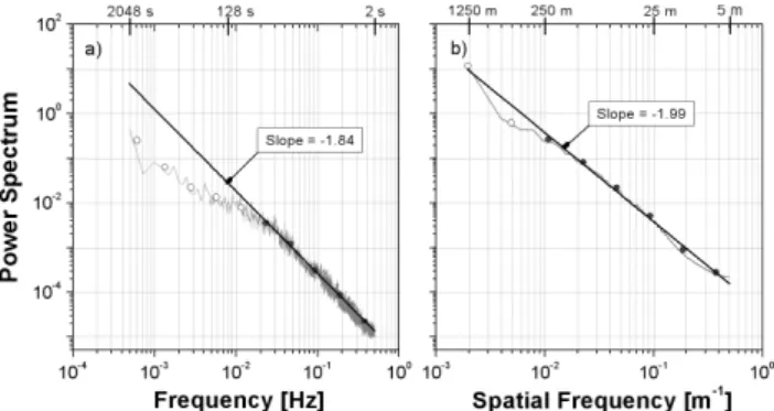
At each point along the distance axis, Fast Fourier Transform algorithm is applied on the time series of the lidar data to obtain the temporal power spectrum. The average temporal power spectrum was estimated by averaging the individual power spectra for the time series corresponding to spatial lo-cations from 150 m to 910 m. The range was selected such that we have continuous time series of lidar-rainfall data. Further, only those individual spectra that display scaling be-havior withR2>0.95 was used to estimate the average spec-trum (Fig. 1a).
We carried out the local linear analysis to check the log-log linearity of the average power spectrum and the departure from scaling behavior. A window, whose size varied loga-rithmically, was moved along the frequency axis of the tem-poral power spectrum and linear regression was performed within that particular window. Logarithmic sized window was selected so that the window size is uniform in a log-log plot. The slope varied from –0.50 to –2.0 with a sharp tran-sition between frequencies corresponding to 80 s and 140 s. From 2 s up to 80 s, the slope varied from –1.75 to –2.0 with a coefficient of variation (CV) of 0.037 compared to the full regime, where the CV was equal to 0.093. Therefore, we can say that the spectrum is log-log linear in the regime 2 s to 80 s
Fig. 1. Temporal and spatial power spectrum of the lidar-rainfall data. The dots indicate the power spectrum averaged in logarithmic (octave) bins. The slope of the regression line fitted to the octave-binned spectrum is also indicated on each panel.
with a departure from scaling around the region 80 s to 140 s (Fig. 1a). The departure could be due to the limited sample of the data resulting in sampling issues towards lower frequen-cies. A thorough analysis with a large dataset is required to check if the scale break (if exists) is related to characteristic time scale in rainfall.
The average spectrum was then octave-binned (e.g., Har-ris et al., 1996) in this region to avoid excessive weighting on higher frequencies, and the regression analysis was car-ried out on the octave-binned spectrum. Figure 1a shows the octave-binned spectrum included in the regression analysis (solid gray circles) along with the fitted regression line. The slope of the regression line fitted to the octave-binned av-erage power spectrum was –1.84 with anR2value of 0.99 (Fig. 1a). Further, the average of the slopes of individual power spectra was equal to –1.81. From these values, it can be said that the average power spectrum is indeed represen-tative of the individual spectra. We refrained from perform-ing linear regression for lower frequencies (empty circles in Fig. 1a) as they are dominated by the sampling effects. Un-like Fabry (1996) and Nikolopoulos et al. (2008), we did not notice any white noise like spectrum at high frequencies. That is, scale-invariance extended up to the scales allowed by the resolution of the data.
4.1.2 Spatial spectrum
256 points most of which were concentrated towards higher frequencies. The average spectrum was octave-binned and the slope was estimated leaving first two points (Fig. 1b). The first two points were not included to avoid sampling ef-fects. The average value of the slopes of individual spatial power spectra was equal to –2.02 and the slope of average spatial power spectrum was –1.99 with anR2value of 0.99. From the high value ofR2, it can be said that the spectrum is log-log linear in the regime 5 m to 250 m. Figure 1b shows the average spatial power spectrum, the octave binned aver-age spectrum and the fitted regression line. It is not possible to compare the spatial power spectrum from this study with the ones reported in the literature as most of them were radi-ally averaged two-dimensional power spectra obtained from two-dimensional rainfall fields.
4.2 Moment scaling
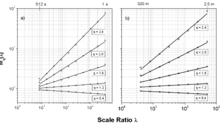
From the Sect. 4.1, we have seen that the power spectral ex-ponents were greater than the dimension of the data, which is one. Therefore, moment scaling analysis was performed on the absolute fluctuations computed using Eq. (2). In the Fig. 2, we show the statistical moments obtained using Eq. (3) for both time and space. It can be noticed that the moments display log-log linearity with respect to the scale. In time, the scale-invariance was found to hold from the low-est resolution of 1 s to 512 s in time and in space it extended from 2.5 m to 320 m. The scaling regimes in time and space were shorter than those noticed in power spectral analysis in the previous section. The power spectrum and the mo-ment scaling analysis are two different tools to investigate the presence of scaling. While the power spectrum is a second-order analysis, the moment scaling invlolves estimation of the moments of order ranging from 0.1 to 3.5. In addition, the sampling issues impact these two techniques in a differ-ent manner. Therefore, the scaling regimes detected by these tools need not be exactly same.
We did not perform the moving window analysis (like in power spectrum) to check the log-log linearity and the devi-ation in scaling behavior as we only had 10 points. TheR2
value for the linear regression in the log-log plot for various moment orders (Fig. 2) was always greater than 0.98. From the high values ofR2, it can be said that the moments are indeed log-log linear. Figure 2 also shows the ordinary least squares regression fit to the statistical moments. The slopes
K(q)of the fitted regression lines are plotted against the cor-responding moment orders for the temporal and spatial do-mains in the Fig. 3. For both cases, the slopes vary non-linearly with the moment order confirming that the rainfall fluctuations are multfractal. Figure 3 also shows the DTM fit and the corresponding universal multifractal parameters for space and time domain. While the intermittency parameter
C1was the same for temporal and spatial data, the
multifrac-tal parameterαwas greater for spatial data (Fig. 3).
Fig. 2.Variation of(a)temporal and(b)spatial moments of rainfall fluctuations of various moment ordersqwith respect to scale ratio
λ. Figure also shows the fitted ordinary linear regression lines.
Fig. 3. Variation of (a)temporal and(b)spatial moment scaling exponents with respect to the moment order. The parameters of the universal multifractal model are given in the inset.
4.3 Dynamic scaling
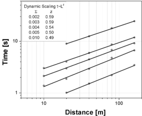
As mentioned in Sect. 3.3, dynamic scaling analysis has to be performed in the region where the statistical properties of the quantity estimated using Eq. (10) do not depend significantly on the absolute time coordinateτ. To identify such stationary region, we moved a window of size 900 s (15 min) along the standard deviation seriesσ 1lnIi,t(8,8)and estimated the CV. The window that resulted in the least CV was selected for the dynamic scaling analysis. The coefficient of variation for the corresponding time period is 0.39. The overall stan-dard deviation6 (L, t )was then estimated for the stationary region for each combination ofLandt. In the Fig. 4, we plot the pairs ofLandt for which the standard deviation6was constant. From the Fig. 4, it can be seen that the relationship betweenLandtis log-log linear confirming the presence of dynamic scaling of the formt∼Lzin the lidar-rainfall data.
Fig. 4. Evidence of dynamic scaling in the standard deviation of
1lnIi,t(L, t )(Eq. 9). The values of the standard deviations and the
corresponding dynamic scaling exponents were given in the inset.
evidence of dynamic scaling in lidar-rainfall (Fig. 4). The scaling range extended from 10 m to 160 m in space and from 1 s to∼20 s in time. However, it should be noted that for a dataset with wider spatial range and longer stationary period, one might notice longer scaling regimes. The dynamic scal-ing exponentzis also shown in the Fig. 4 along with the cor-responding standard deviations. The value ofzvaried from 0.49 to 0.59 depending on the standard deviation. The ex-ponents were different compared to Venugopal et al. (1999) who reported exponents in the range of 0.6 to 0.7 for tropical convective storms of Darwin, Australia. The scaling regimes from this study cannot be compared with that of Venugopal et al. (1999) as they analyzed radar-rainfall images with a resolution of 2 km in space and 10 min in time.
5 Summary and conclusions
We investigated the space-time lidar-rainfall data with a res-olution of 2.5 m in space and 1 s in time for the presence of scale invariance. The power spectrum analysis suggested that the lidar-rainfall data were scale-invariant with exponents of –1.84 and –1.99 in time and space respectively. The scal-ing regime in time extended from 2 s up to 80 s. We noticed a transition region between 80 s and 140 s, where the power spectrum departs from the scaling behaviour. The scaling regime in space extended from 5 m to 250 m. We did not ob-serve white noise spectrum at higher frequencies that were reported by some previous studies. In the moment scaling analysis, the statistical moments of the rainfall fluctuations displayed scaling behaviour with scaling regimes extending from 1 s to 512 s in time and 2.5 m to 320 m in space. The nonlinearity of the moment scaling function indicated that the lidar-rainfall data displayed multiscaling behaviour both in space and time. TheK(q)function was then
paramete-rized according to the double trace moment technique to ob-tain the universal multifractal model parameters. The inter-mittency parameterC1was same for both spatial and
tempo-ral lidar-rainfall series. The multifractal indexαwas equal to 1.92 for temporal and 1.97 for spatial data. The values of α indicate that the lidar-rainfall data corresponds to the log(Levy) multifractals. We also noticed a space-time trans-formation of the formt∼Lzin the lidar-rainfall data with an exponent in the range of 0.49 to 0.59. However, it should be noted that this transformation was observed only for the very small scales in the range of 1 s to∼20 s in time and from 10 m to 160 m in space.
Our high-resolution dataset allowed us to perform multi-scaling analysis at very small scales that received little at-tention in the literature. However, to really bridge the scale gap, we need to perform an expensive experiment with li-dars, rain gauges, radars and satellites observing the same rainfall system for a considerable time period. Such an exper-iment should be designed so that there is some overlap in the scales observed by different instruments. Besides bridging the scale gap, such an experiment will also provide insights into the physical mechanisms responsible for the observed scaling behavior in rainfall datasets.
Acknowledgements. The authors acknowledge useful discussions with Deborah Nykanen and V. Venugopal.
Edited by: J. Kurths
Reviewed by: two anonymous referees
References
Crane, R. K.: Space-time structure of rain rate fields, J. Geophys. Res., 95, 2011–2020, 1990.
Desaulniers-Soucy, N., Lovejoy, S., and Schertzer, D.: HYDROP experiment: an empirical method for the determination of the continuum limit in rain, Atmos. Res., 59–60, 163–197, 2001. Fabry, F.: On the determination of scale ranges for precipitation
fields, J. Geophys. Res., 101, 12819–12826, 1996.
Georgakakos, K. P., Carsteanu, A. A., Sturdevant, P. L., and Cramer, J. A.: Observation and analysis of Midwestern rain rates, J. Appl. Meteorol., 33, 1433–1444, 1994.
Gupta, V. K. and Waymire, E. C.: A statistical analysis of mesoscale rainfall as a random cascade, J. Appl. Meteorol., 32, 251–267, 1993.
Harris, D., Menabde, M., Seed, A., and Austin, G.: Multifractal characterization of rain fields with a strong orographic influence, J. Geophys. Res., 101, 26405–26414, 1996.
Lewandowski, P., Eichinger, W. E., Kruger, A., and Krajewski, W. F.: Lidar-based estimation of small-scale rainfall: empirical evi-dence, J. Atmos. Ocean. Tech., 26, 656–664, 2009.
Lilley, M., Lovejoy, S., Desaulniers-Soucy, N., and Schertzer, D.: Multifractal large number of drops limit in rain, J. Hydrol., 328, 20–37, 2006.
Lovejoy, S. and Schertzer, D.: Multifractals, cloud radiances and rain, J. Hydrol., 322, 59–88, 2006.
Lovejoy, S., Schertzer, D., and Allaire, V. C.: The remarkable wide range spatial scaling of TRMM precipitation, Atmos. Res., 90, 10–32, 2008.
Marsan, D., Schertzer, D., and Lovejoy, S.: Causal space-time mul-tifractal proceses: Predictability and forecasting of rain fields, J. Geophys. Res., 101, 26333–26346, 1996.
Menabde, M., Seed, A., Harris, D., and Austin, G.: Self-similar ran-dom fields and rainfall simulation, J. Geophys. Res., 102, 13509– 13515, 1997a.
Menabde, M., Harris, D., Seed, A., Austin, G., and Stow, D.: Multi-scaling properties of rainfall and bounded random cascades, Wa-ter Resour. Res., 33, 2823–2830, 1997b.
Nikolopoulos, E. I., Kruger, A., Krajewski, W. F., Williams, C. R., and Gage, K. S.: Comparative rainfall data analysis from two vertically pointing radars, an optical disdrometer, and a rain gauge, Nonlin. Processes Geophys., 15, 987–997, 2008, http://www.nonlin-processes-geophys.net/15/987/2008/. Nykanen, D. and Harris, D.: Orographic influences on the
mul-tiscale statistical properties of precipitation, J. Geophys. Res., 108(D8), 8381, doi:10.1029/2001JD001518, 2003.
Olsson, J., Niemczynowicz, J., and Berndtsson, R.: Fractal analy-sis of high-resolution rainfall time series, J. Geophys. Res., 98, 23265–23274, 1993.
Perica, S. and Foufoula-Georgiou, E.: Model for multiscale dis-aggregation of spatial rainfall based on coupling meteorological and scaling descriptions, J. Geophys. Res., 101, 26347–26361, 1996.
Schertzer, D. and Lovejoy, S.: Physical modelling and analysis of rain and clouds by anisotropic scaling multiplicative processes, J. Geophys. Res, 92, 9693–9714, 1987.
Tessier, Y., Lovejoy, S., and Schertzer, D.: Universal Multifractals: Theory and observations for rain and clouds, J. Appl. Meteorol., 32, 223–250, 1993.
Veneziano, D., Bras, R. L., and Niemann, J. D.: Nonlinearity and self-similarity of rainfall in time and a stochastic model, J. Geo-phys. Res., 101, 26371–26392, 1996.