Variability in Regularity: Mining Temporal Mobility Patterns in London, Singapore and Beijing Using Smart-Card Data.

Variability in Regularity: Mining Temporal

Mobility Patterns in London, Singapore and

Beijing Using Smart-Card Data

Chen Zhong1*, Michael Batty1, Ed Manley1, Jiaqiu Wang1, Zijia Wang2,3, Feng Chen2,3, Gerhard Schmitt4

1Centre for Advanced Spatial Analysis, University College London, London, United Kingdom,2School of Civil and Architectural Engineering, Beijing Jiaotong University, No.3 Shangyuancun, Haidian District, Beijing, P. R. China,3Beijing Engineering and Technology Research Centre of Rail Transit Line Safety and Disaster Prevention, No.3 Shangyuancun, Haidian District, Beijing, P. R. China,4Future Cities Laboratory, Department of Architecture, ETH Zurich, Zurich, Switzerland

*c.zhong@ucl.ac.uk

Abstract

To discover regularities in human mobility is of fundamental importance to our understand-ing of urban dynamics, and essential to city and transport plannunderstand-ing, urban management and policymaking. Previous research has revealed universal regularities at mainly aggregated spatio-temporal scales but when we zoom into finer scales, considerable heterogeneity and diversity is observed instead. The fundamental question we address in this paper is at what scales are the regularities we detect stable, explicable, and sustainable. This paper thus proposes a basic measure of variability to assess the stability of such regularities focusing mainly on changes over a range of temporal scales. We demonstrate this by comparing reg-ularities in the urban mobility patterns in three world cities, namely London, Singapore and Beijing using one-week of smart-card data. The results show that variations in regularity scale as non-linear functions of the temporal resolution, which we measure over a scale from 1 minute to 24 hours thus reflecting the diurnal cycle of human mobility. A particularly dramatic increase in variability occurs up to the temporal scale of about 15 minutes in all three cities and this implies that limits exist when we look forward or backward with respect to making short-term predictions. The degree of regularity varies in fact from city to city with Beijing and Singapore showing higher regularity in comparison to London across all tempo-ral scales. A detailed discussion is provided, which relates the analysis to various character-istics of the three cities. In summary, this work contributes to a deeper understanding of regularities in patterns of transit use from variations in volumes of travellers entering subway stations, it establishes a generic analytical framework for comparative studies using urban mobility data, and it provides key points for the management of variability by policy-makers intent on for making the travel experience more amenable.

OPEN ACCESS

Citation:Zhong C, Batty M, Manley E, Wang J, Wang Z, Chen F, et al. (2016) Variability in Regularity: Mining Temporal Mobility Patterns in London, Singapore and Beijing Using Smart-Card Data. PLoS ONE 11(2): e0149222. doi:10.1371/journal. pone.0149222

Editor:Tobias Preis, University of Warwick, UNITED KINGDOM

Received:November 24, 2015

Accepted:January 28, 2016

Published:February 12, 2016

Copyright:© 2016 Zhong et al. This is an open access article distributed under the terms of the

Creative Commons Attribution License, which permits unrestricted use, distribution, and reproduction in any medium, provided the original author and source are credited.

Data Availability Statement:Data are available from the Transport for London (TFL) in UK, Land Transport Authority (LTA) in Singapore and Beijing Transport Committee in China for researchers who meet the criteria for access to confidential data.

Introduction

Urban mobility shapes space as much as space shapes urban mobility [1]. To find regularity in human mobility is of fundamental importance to a better understanding of urban dynamics and this yields insights into extensive applications varying from urban transportation [2–4], social structure [5], and urban design [6–8] to epidemiology [9,10] and urban infrastructure [11]. Urban dynamics can be characterised by mobility patterns at different scales. In terms of the temporal dimension, allometric scaling laws for city size have been discovered from long-term population data [11–13], while patterns of spatial interaction have been explored and modelled over long-time periods and for long-distance movements between cities [14] using power laws.

Urban mobility data has exploded in recent years as data sets pertaining to transactions and movement in real time from mobile phones, GPS tracking, Wi-Fi, smart cards, and social media give much finer granularity of detail. This has greatly promoted the discovery of many different kinds of regularities, adding new perspectives to classical scaling laws and theories, especially for short-term movements at an individual level. For instance, Gonzalez et al [15] tracked anonymised mobile phone users for six-months, finding, in contrast to the random tra-jectories predicted by the prevailing Levy flight and random walk models, a high degree of spa-tiotemporal regularity exists in human trajectories. Schneider et al [16] constructed networks of individual daily mobility from two types of data, namely mobile phone data in Paris and trip survey data in Paris and Chicago, finding 17 unique motifs that all follow simple rules useful for modelling and simulation. Other work using multi-source data including taxi data has sug-gested that as population density decreases exponentially with distance from the urban centre, this ultimately leading to an exponential law of collective intra-city mobility [17].

There are also studies using smart card data, a comparatively new type of data generated by Smart Card Automatic Fare Collection (SCAFC) systems. These data have revealed diverse fea-tures about mobility that have not been possible to observe hitherto. The small world phenom-enon, for example, has been found in daily encounters relating to shared bus travel establishing certain probabilities of meeting“familiar strangers”[18]. A similar phenomenon has been found in the geographic circulation of banknotes in the United States [19]. Other data sets form social media sites such as Foursquare [20] differ from data where mobility is directly deterred by the costs associated with physical distance, generating scaling laws that are consis-tent with intervening opportunities, built on rank-distance instead of pure physical distance.

Though progress has been made in revealing different perspectives on regularity as well as adding variability at finer scales to classical universal scaling laws, the statistical structure of human mobility is still far from predictable. High degrees of regularity emerge mostly at aggre-gated levels either for large population groups or for long-term changes. Detected preferences for movements at fine scales against more simplistic laws of motion already demonstrate the existence of such variability and this has been briefly addressed in recent work [15,20,21]. At a disaggregate level, diversity appears due to increasingly complex causal factors. Song et al [22] raise a fundamental question as to what degree is human behaviour predictable from investiga-tions of the stability of predicinvestiga-tions by measuring the entropy of individual trajectories. Factors such as travel time, sample size, as well as demographic structure are discussed to explain these entropy values. In the light of the insights gained in this research, we hypothesize that in the context of urban mobility, the degree of regularity decreases across all scales, specifically, spa-tial and temporal scales, and aggregations of different factors that condition mobility itself, and thus follow certain functions that can be detected, represented and then modelled.

Here we raise three questions. First at which aggregated scales does regularity persist? Sec-ond if certain changes in regularity occur, does this occur randomly or does it scale in a regular

design, data collection and analysis, decision to publish, or preparation of the manuscript.

way? Third, does urban context matter? This paper investigates such‘variability in regularity’ with a primary focus on temporal scales. The reason we begin with the temporal dimension is to make use of the distinctive advantages of smart-card data, which enable us to look into urban mobility down to the scale of one-minute granularity, which is as detailed as any analysis of such urban phenomena to date.

We first need to clarify definitions. Byregularity, we mean a uniform pattern, principle, arrangement, or order that repeats itself, is reproducible, and therefore can be used as basis for urban and transport simulation and prediction. Bytemporal scale, we mean the minimum tem-poral unit for data aggregation, which implies how far one is able to look at the temtem-poral series backwards and forwards. We will propose a method to quantify the stability of any form of reg-ularity identified by measuring variability over different temporal scales. The method is applied to smart-card data, which has wide demographic and geographic coverage of urban mobility. We use this variability in regularity as an index for comparative study using one-week’s worth of smart-card data from our three candidate cities, namely London, Singapore and Beijing. On the one hand, our purpose is to demonstrate the existence of universal regularity as variability changes; on the other, our approach serves as a common analytical framework for comparing regularities in human mobility, relating any variability to related characteristics of cities.

Methods: A Basic Measure of Regularity

We give scope to this work by evaluating the stability of regularity in the temporal dimension through measuring the variability of mobility patterns over multiple days. We assume here that the units associated with regularity could be any elements or objects that are associated with urban mobility, such as individual passengers, trains, stations, flows and so on. Accordingly, a set of attributes will be defined to characterize a specific regularity; for instance, travel purpose for a person, capacity and speed for a train, transfer flows for a station, and so on. Although our comparative studies in later sections use stations as study subjects specifically, we will also generalise our method to flow systems that depend on trips between origins (O) and destina-tions (D). The method we propose is thus generic and applicable to many conceptualisations and aggregations of our basic data sets.

2.1 Definitions and Notation

Urban mobility can be decomposed and evaluated in terms of different objects, such as a travel-ler, a station, an area associated with a station, or a fixed transit line or route. An object with finite measurextcan be written as a vectorxN(i)

xNðiÞ ¼ ½x1;x2;x3;. . . x_t;. . . x_nŠ ð1Þ

wherextis a measure of the objectN, say a station, at time slott,t2[1,. . .,n] andnis the num-ber of sequenced time slots; [x1,x2,x3,. . .xt,. . .xn] is thus the temporal pattern of the object

xN(i) which depends on the number of time slotsnthat define a day. Moreover,idenotes the day on which the temporal pattern is measured. A stable and reliable regularity would thus exist with respect to this profile over days implying thatxN(i)*xN(j),i6¼j. The objective of our analysis is to assess the variability ofxN(i) between multiple days. Note that the indexN characterises the object in question that might be a set of stations or a set of travellers and it is clear enough that we do not need to notate each element of this vectorxtwith respect to its objectNor dayi.

smart card could further decompose the number of passengers intomattributes and in this way we might define a matrixXN(i) as

XNðiÞ ¼

x11;x12;x13;. . . x1t;. . . x1n

x21;x22;x23;. . . x2_t;. . . x2_n

x31;x32;x33;. . . x3t;. . . x3n

: : :

xm1;xm2;xm3;. . . xmt;. . . xmn 2 6 6 6 6 6 6 6 4 3 7 7 7 7 7 7 7 5

ð2Þ

where each column is the vector associated withxtin Eq (1) above. To repeat the limits,Nis the object type,iis the day,nis the number of sequenced time slots, andmis the attribute of the element defined at the time slot in question. In the sequel, we assume that the time slots are in minute intervals, the attributes are the types of travel such as theflow from one station to another, the objects are defined with respect to the station they profile, and the day of the week for this profile defines the station and the elements of the matrixXN(i). We should also note that Eq (2) is a generalisation of Eq (1) in that if, then the problem collapses to one where we are examining variations across attributes of passengers. Whenm= 1, the variation is across temporal intervals.

2.2 Measuring Accumulated Variability

We first consider the vectorxN(i) which we will use to measure the relative variance of each dis-tribution over multiple days. Since there is no baseline for comparison, we compute the vari-ability between any two distributions for each of two separate days. Regularity exists only when the variance between any two distributions is low, and we will reject the hypothesis that there is strong regularity if the detected temporal patterns across certain time units are unstable over multiple days. We measure this degree of regularity from the correlation between any two days

iandj,i6¼jwhere we generate the correlation betweenxN(i) andxN(j) from the normalised covariance matrix formed from these vectors. This gives the correlation matrixr(i,j) from which we can gauge the degree of regularity between any two days.

The square of these valuesr2(i,j) is the amount of covariance that is explained by the corre-lation where, for example, if this is 0.6, then this means that 60% of the variation between any two patterns or profilesxN(i) andxN(j) is common and the remaining 40% is not. Clearly in this context, we are looking for comparisons where ther2(i,j) values are as high as possible. Since variance between any two days is what matters, we can calculate the accumulated vari-ance, which we define as the variability statistic as:

CVar¼X

l

i¼1 Xl

j¼iþ1

ð1 _r2_{ði;jÞÞ=ðlðl} 1_Þ=2_{ÞÞ ð3Þ}

where the summations are overldays, normalized by (l(l−1)/2)) which is the number of comparisons.

variability of individual observations decreases due to averaging of the data. Given this deter-minant of variability, we are searching for deviations from this pattern between days and between cities and dependent on causal determinants related to when people travel, then the variability measureCVarin Eq (3) will detect such differences. The deviations/variability deter-mines to what extend history trip data can be used for real-time trip prediction, which is crucial for passenger management, and transit planning.

Data and Applications

Our comparative study of temporal urban mobility patterns using the proposed variability has been developed for three large cities, namely London, Singapore, Beijing, all of which have available smart-card data for at least one week. The smart-card data is generated by various Smart Card Automated Fare Collection (SCAFC) systems, which were originally designed to collect revenue for better financial management and accounting for public transportation systems. These also produce large volumes of data about boarding and alighting from the vehi-cles or trains which in the case of the smart-card involve tap-ins and tap-outs by the traveller [23–25].

The quality of smart-card data varies from city to city in term of the richness of the informa-tion available, the coding system adopted, and the granularity and completeness of data, but in this analysis, we have only used the basic information including station code and time tag when boarding or alighting occurs. This basic information is captured in almost all the cities for which smart-card data is available, and this implies that this comparative study can be easily expanded.

We will note the key characteristics of the three cities and their transit systems before we begin the analysis. London’s population, which is directly served by the subway and related transit systems, was about 8.6 million in 2014 and its metro system is the oldest rapid transit system in any city, and being first constructed as an underground heavy rail system in the 1860s. The London Travel Demand Survey (LTDS) reports that around 30% of total popula-tion in the Greater London area use public transportapopula-tion for their daily commuting [26]. The smart card data is recorded by London’s Oyster card system which is used by approximately 90% of bus passengers and 80% of rail passengers [27]. The trains dataset contains approxi-mately 9 million transactions daily, which are entry/exit transactions associated with the train systems (Underground (Tube), Overground and Docklands Light Railway (DLR)). Both entry and exit data are available for train rides at gated stations, while only entry data is available for bus rides. During the period of analysis, the London Underground network had 13 lines with 400 stations in use detected from the smart-card data available for a week in February 2014.

Singapore, our second example is an island city-state with a current population of approxi-mately 5.3 million of whom about 62% (or 3.29 million) are residents, the rest being foreign workers or their dependents, according to the 2012 census. The metro system called the Mass Rapid Transit (MRT) system in Singapore, has 102 subway stations with several new lines opening in the last five years. At present the land-based public transportation system in Singa-pore comprises two networks: the MRT and the bus system with more than half the population using public transportation as their main transport mode [28]. The collected tap-in/tap-out events provide a huge data set with around 5 million daily travel records, which we have been able to access as smart card data provided by the Singapore Land Transport Authority. This study was conducted using the available smart-card data from the EZ-Link system for one week in March 2013.

considerations and was open for citizens years later. It has undergone rapid expansion since the end of the 29th summer Olympic Games in 2001. New lines begin operating almost every year. The trip share of metro soar from 3.6% in 2000 to 20.6% in 2013, and is expected to con-tinue to increase. Beijing’s population had reached 21 million by the end of 2013 but a consid-erable part of the city is not developed being rural and mountainous areas (Beijing Traffic Development Research Centre, 2014). The service area of the metro network in fact is circled by the 6th ring road, and this reduces the population served by the system to some 5 million. The mode share of the metro is 21% without walking trips and the data used for this analysis is based on data from the Yikatong card which accounts for 85% of the total trips made on the network. Although a simple flat fare is applied to the network, passengers need to use their cards to tap in and tap out with two records being logged for each metro trip. The original card transaction data generated on the Beijing metro network were made available for October 2014 by the Beijing Municipal Commission of Transport.

The differences reflected inTable 1are considerable and before the analysis, we had little idea of the degree to which travel behaviour on these respective subway systems would differ. London’s much older system where there is less scope for new lines than in Singapore contrasts with the Beijing system, which is quite old but has received considerable enhancement in recent years. This is reflected to an extent in usage with the highest usage rate in terms of ridership and mode share in Singapore (35% according to [29]).

Experiments and Outcomes

In our experiments, we take the metro station as the basic urban element or object and study the regularity of temporal urban mobility patterns at each station during one-week (5 week days) based on the availability of data in all three cities. Weekends are excluded since huge vari-ability exists on Saturdays and Sundays due to the fact that work and leisure activities differ most during these periods due to cultural factors [30].

We have developed two experiments demonstrating the usage of vectorxN(i) and matrix

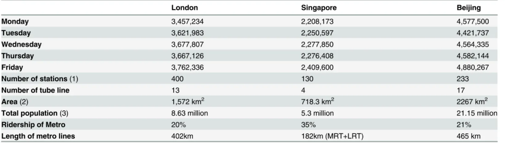
XN(i) respectively to measure the regularity at different scales with respect to when and where people travel. In our first experiments, we examine when people travel. More specifically, this is about the temporal distribution of trip starting times during one week. In this context, the Table 1. Summary statistics of one-week of smart-card data (metro trips only).

London Singapore Beijing

Monday 3,457,234 2,208,173 4,577,500

Tuesday 3,621,983 2,250,597 4,421,737

Wednesday 3,677,807 2,277,850 4,564,335

Thursday 3,667,126 2,276,408 4,582,144

Friday 3,762,336 2,409,600 4,880,267

Number of stations(1) 400 130 233

Number of tube line 13 4 17

Area(2) 1,572 km2 _{718.3 km}2 _{2267 km}2

Total population(3) 8.63 million 5.3 million 21.15 million

Ridership of Metro 20% 35% 21%

Length of metro lines 402km 182km (MRT+LRT) 465 km

(1) Number of stations is the number of stations with smart-card records generated.

(2) The area of Beijing only counts the area enclosed by the 6th ring road for a fair comparison.

(3) From the World Population Review,http://worldpopulationreview.com/world-cities/accessed 05 February 2016

regularity is about temporal patterns of traffic flow, thus, an individual measurextis a single value, which is the gate count. Therefore, we can then derive the definition from the generic vectorxN(i). We definefN(i) = [f1,f2,f3,. . .,ft,. . .,fn] whereftis the number of people starting a trip at a stationNduring time slott. The total number of time slotsnis determined on a time interval, which is defined to aggregate the basic minute by minute data. For instance, if the time interval is set to be 12 hours, thenn= 2 because a day will be divided into two time slots. Note that there are 1440 minutes in a day and the time interval for dividing a day in 2 would be of 720 minutes duration.

The second experiment conflates the data to deal with flows between origins and destina-tions, which are associated with each stationN. In this case, an individual measurexthas more than one attribute, which are interchange flows between any pair of stations. The regularity is therefore based on spatial patterns of trips, which originate and are destined for each station. We then derive the definition from the generic matrixXN(i). Each measureftis a vector com-posed by 2(M−1) attributes that are volume of passengers flowing from the given stationNas

an origin to all other stations and from all other stations to the destination stationNin ques-tion for a given dayi. Following Eq (2), we can write this matrix as

FNðiÞ ¼

fN;1; f_N;2; f_N;3;. . . f_N;t;. . . fN;n

fN 1_;1; f_N 1_;2; f_N 1_;3;. . . f_N 1_;t;. . . f_N 1_;n

fN 2;1; f_N 2;2; f_N 2;3;. . . f_N 2;t;. . . fN 2;n

: : : : :

fM;1; fM;2; fM;3;. . . fM;t;. . . fM;n

: : : : :

fM;1; fM;2; fM;3;. . . fM;t;. . . fM;n

fM 1_;1; f_M 1_;2; f_M 1_;3;. . . f_M 1_;t;. . . f_M 1_;n

fM 2;1; fM 2;2; fM 2;3;. . . fM 2;t;. . . fM 2;n

: : : : :

fN;1; fN;2; fN;3;. . . fN;t;. . . fN;n 2 6 6 6 6 6 6 6 6 6 6 6 6 6 6 6 6 6 6 6 6 6 6 6 6 4 3 7 7 7 7 7 7 7 7 7 7 7 7 7 7 7 7 7 7 7 7 7 7 7 7 5

: ð4Þ

This matrix is arranged so that the columns represent the outflow of passengers from one sta-tionNto all other stations up toMand the inflow from all other stations starting fromMto the station in questionNwhere the rangeN. . ._{Mis the outflow and the rangeM}. . ._{Nis the inflow. In} short for each time interval, we have a vector of length 2(M−1) where the number of stations is Mand the self flows from a station to itself are also counted. The first part of the column vector in the matrix is the outflow and the second part the inflow, thus accounting for all flows from and two each station in question. The matrixFN(i) are these flows for a particular station and the matrix is thus a measure of the variability over all time periods and over all flows to all stations for a particular station in question. A comparison of matricesFN(i) andFN(j) for each station pro-vides the variability at this more detailed level of trip flows. There flows represent the trips from an origin station to all its destinations and from these destinations back to the origin station.

here are thus defined as intervals of 1440, 720, 360, 96, 80, 60, 45, 30, 20, 15, 8, 4, 2, and 1 min-utes which yieldn= 1,2,4,15,18,24,32,48,72,96,180,360,720,1440 numbers of elements. The rationale for this sequence is to keep the intervals as close as possible to some exponentially increasing function of time over the range from 1 to 1440 minutes.

4.1 Variability Increases on Lower Temporal Scales

When and where people travel to is the most fundamental information that can be extracted from urban mobility data and plots of temporal distributions with respect to when a trip starts or ends can be found in most of the results from mobility data analysis [31,32]. Usually very regular distributions over multiple weekdays can be easily be spotted with very similar flow vol-umes especially at peak hour times. The O-D matrix is also another frequently used plot for transit planning, which is used in estimating flows between locations. Both temporal distribu-tions and the O-D matrix profiles can be generated at different temporal scales. As indicated earlier, the choice of different scales implies how far one is able to look back and how far for-ward or ahead. Using this focus on temporal scales, we can interpret the results from our analy-sis in terms of four related questions based on 1) how does regularity change at each temporal scale? 2) how does regularity change across temporal scales? 3) how does regularity vary within each temporal scale? and 4) how easy is it to predict destination choices of trips at any time of the day? We pose these questions rhetorically and answer them in turn.

4.1.1 Does detected regularity sustain at all temporal scales?. The degree of regularity

clearly decreases as the temporal dimension gets larger, that is as the scale gets coarser.Fig 1is a plot of the normalised variabilityCVarof all measures for all stations using defined time intervals from 1 minute to 12 hours which are displayed left to right on x-axis. A higher vari-ability means less regularity, in other words, the regularity becomes more difficult to predict with accuracy.Fig 2also shows that the variability increases along with increasing temporal resolution. This is in line with our notion that passengers arrive at stations randomly with respect to their decision to travel and this is a product of human decision, congestion at the gate, bad weather, and human frailties in terms of keeping to their schedules and so on.

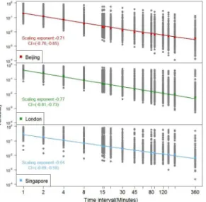
4.1.2 How does the detected regularity change across temporal scales?. If we arrange the

scales from the smallest to the largest as inFig 1, the variability decreases in a regular fashion following a non-linear function, which we show inFig 2where the vertical scale is logged to assess the degree of linearity. Here we show this for the three cities London, Singapore, and

Fig 1. Variability of temporal patterns of trip starting times on the London underground.

Beijing and this implies that the same kind of exponential decrease in variability occurs that we see inFig 1for Singapore and Beijing. London has the steepest scaling exponent of -0.772 whereas Singapore has the lowest scaling -0.645 but the differences do not appear particularly significant. Note that inFig 2, the median value ofCVaris plotted as are all other values for each of the metro stations for each city. The median values are then used to fit the linear rela-tions over the 17 time intervals in question and it is clear that the relarela-tions are essentially non-linear reflecting the consistency withFig 1, which just shows the London underground.

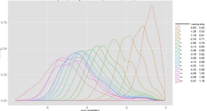
4.1.3 At each temporal scale, how does variability in regularity vary?. Fig 3plots out the

density distributions with respect to the variability of all 400 stations measured at different temporal scales for London. Different colours denote measurements at different time intervals. These density distributions of the variances associated with stations imply less variance as the temporal scale increases and is consistent withFig 2while this log normality is consistent over all scales. These results partially prove our hypothesis that regularity can always be found at the aggregated level while diversity appears at the disaggregate.

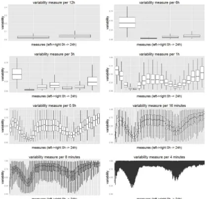
4.1.4 Can we predict the variability of all trips at all times of a day?. This question

con-cerns the variability of trips at different stations at different times of the day. This is important because the data that forms the essence of the Origin-Destination (O-D) matrix for estimating traffic flows is an important problem where smart-card data has already been used implying a fair degree of accuracy [27,33]. In the same way that we examined changes in overall variability with respect to different temporal scales, the variability of trips at each time of the day clearly gets larger for finer temporal scales and this is clearly shown inFig 4. Moreover, the variability of trips during different times of the day implies different distributions. Morning and evening peak hours have a comparatively lower variability across all measures. In other words, trips in the peak hours are most regular and thus more predictable probably because most of them are home-work based trips that have fixed origins and destinations. We thus conclude that the dis-tribution of trips can be predicted at aggregated levels but only for specific periods of a day, namely the peaks. To an extent, this demonstrates that focusing transport models on predicting peak hour flows is statistically more robust than using them for prediction at other times of the day.

Fig 2. Variability as a function of the time intervals for London, Singapore, and Beijing.Note: The negative linear relations show that the variability declines with increasing temporal scale but the variations in the variability (the variance of the covariance) which relate to the stations also increase for all three cities.

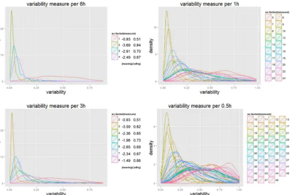
As inFig 3, we also plot out the density distributions of variability for the 400 London underground stations, which we show inFig 5. The four plots are taken from results for the 6 hour, 3 hour, 1 hour, 0.5 (half) hour time intervals respectively. These distributions for the dif-ferent time slots are shown in difdif-ferent colours. A lognormal like distribution can be found for all measures, with smallest variance values at the morning and evening peaks.

4.2 Regularity Rankings for London, Singapore and Beijing

We directly compare the three cities in this section, plotting the variability for these inFig 6 The different sizes of metro system as well as the population of passengers have no influence on the variability measure, which is always normalized within [0,1] as is clear fromFig 6that is another form ofFig 2. This shows that the Beijing metro system, although it moves the largest number of passengers and has the largest average flow per metro station, has the smallest vari-ability across all measures. This means the flow volume in the Beijing underground is compara-tively more predictable than others with Singapore in second place while it is clear that in London, this kind of travel is more difficult to predict.

It is possible that the complexity of the metro system might generate higher variability. From casual evidence of knowing the three systems, metro traffic on the London underground is quite often influenced by disruption such as signal failures and strike days. This could par-tially explain the larger variability of temporal patterns in that passengers stagger their journeys more than in other systems. The local demographics of passenger types could be another rea-son for all those who are 60+ years who reside in London can receive a free pass and this adds to greater variability particularly outside the peak hours. Moreover, these three cities are global cities which have large number of visitors and tourists contributing to a larger number of irreg-ular, non-routine trips.

Fig 3. Distribution of the variability of trip starting time at London underground stations.Note: Less variance as the temporal scale gets finer while log normality is consistent over all scales.

In terms of origins and destinations of trips, we plot the percentage of‘predictable’stations inFig 7. These are stations with variability smaller than a valueCVarcutoffat any measured time slot of a day. We then plot the percentage of predictable stations (Npredictable/Ntotal) with

CVarcutoff= 0.1 andCVarcutoff= 0.25. The percentage increases as the time intervals are aggre-gated. When the overall variability decreases along with increasing temporal scale as men-tioned earlier, more stations fulfil the conditionCVarcutoff<0.1 andCVarcutoff<0.25.

Although our goal is to characterize different cities and to determine if a universal pattern is found using these two sets ofCVarcutoffvalues, a critical point exists at 15 minutes, which implies how closely we can predict future events. Because the variability of the trip matrix increases sharply as the time slot decreases to less than 15 minutes, it is impossible to estimate where passengers travel unless further information on individual identification is considered even though real-time boarding information is captured at fare gates. It is a coincidence that the critical time slot obtained here is the same as the generally applied time interval for calcu-lating the peak hour factor (PHF) originally proposed in highway engineering [34]. PHF is an indicator of the irregularity of peak hour demand, normally calculated as 4 times the 15 min peak in peak demand divided by the peak hour demand. This factor is important because trans-port infrastructure is usually designed using peak hour demand and its variability. As the head-ways of new heavy rail systems decrease to less than 2 minutes, it is reasonable to scale down the time interval to address short-term irregularity. Our results demonstrate that it is rather difficult to extract a stable PHF at a higher time resolution than 15 minutes.

We further extend the way we define predictable stations using a ranking mechanism. Sta-tions become more predicable in terms of trip flows at higher temporal resoluSta-tions and these Fig 4. Variability of regularity in the trip matrix over time.Note: Each box plot shows the variability of 400 stations over time measured at different temporal scales. Overall, eight subplots give a similar trend where lower variability appears during peak hours (around 9 am in the morning and 6pm in the evening). More details can be captured as differences of variability between each time unit are magnified as we decrease the temporal scale from 12h to 4 minutes.

get a higher ranking. Both temporal patterns of trip starting timesRstarting–timeand trip location patternsRO–Dare ranked at five levels as shown inFig 8(left). A combined rank is calculated as

Rcombined= min{Rstarting–time,RO–D} and mapped inFig 8(right). Both the statistical and geo-graphical distributions of predictable stations are shown.

When we compare the three cities, we find that London is the most unpredictable of the three in terms of time, origin and destination of trips. The very dense distribution of metro sta-tion in the central area could well be the reason for many people have more than one choice of station for their journey and often this does not make a significant difference to their travel Fig 5. Densities of variability for different time intervals for 400 London underground stations.Note: Less variance exists at a certain time slot, while log normality is consistent over all time slots at all scales. More details about the differences show up when the temporal scale decreases.

doi:10.1371/journal.pone.0149222.g005

Fig 6. Comparative analysis of variability in temporal patterns.

time. We are able to extract from the Oyster card data that many people take alternative routes, in particular for home-work trips and vice versa. Passenger management measures could well be another reason. For example, closing some of the fare gates at Bank and Camden Town, temporally holding passengers back from entering the station at Finsbury Park, closure of Fig 7. Comparative analysis of predictable trips origin and destinations.Note: A critical point exists at 15 minutes in all three cities as a universal pattern, which implies how closely we can predict future event.

doi:10.1371/journal.pone.0149222.g007

Fig 8. Combined ranking of when and where people travel.Note: Stations are ranked byCVarcutoff= 0.1

and measured using temporal scales = 4, 15, 30, 60 and 180 (minutes). Stations which fulfill conditions at 4 minute temporal scales get the highest rank as 5 and so on. The geographic mapping is color coded by a combined score.

Victoria and Oxford Circus due to congestion at certain periods are frequently cited events that pertain to limits on capacity. These measures definitely increase the degree of irregularity in trip patterns

On the contrary, Singapore is the most predictable city in that its relatively simple and newer tube network is seldom affected by accident or train and signalling disruptions, and its planned polycentric urban form appears to produce a more smoothly flowing system than Lon-don. Sub-centres are built along the metro stations and surrounded by residential locations. Therefore, the choice of metro stations from which to travel is mostly influenced by relative distance and not so many alternative directions of travel on different lines are possible.

Beijing however has the highest regularity with respect to its temporal distribution of trips and is second with respect to station location. A number of reasons contribute to this. The most important one is the regular passenger control measure which is applied to about 40 sta-tions where passengers are held outside the stasta-tions before being allowed to enter at regular time intervals during the morning peak. Such queues can last for miles. Passengers can either wait there, search and use an alternative station or mode according to their situation. This mea-sure increases the temporal regularity by interfering with the randomness of arrival times and it decreases spatial regularity by forcing people to change their boarding stations randomly. Moreover, this inconsistency of temporal and spatial regularity can also ascribed to another unique phenomena in Beijing which is due to Vehicles Plate Number Traffic Restriction Mea-sures (note: The restriction is based on the last digit on the license plate. For example, vehicles with a last plate digit of 2 or 7 must be off the road on Monday. Details of the restriction can be found in a bulletin posted on the website of the Beijing Traffic Management Bureauhttp:// www.bjjtgl.gov.cn/) where many private car owners drive a car on most days but for one day use public transport system.

Discussion and Conclusion

Here we have proposed a simple variability measure based on computing simple variances between any two profiles for detecting regularities and of metro trips associated with station and times of travel for three of the largest metro systems in world cities. This measure can be further used as part of an analytical framework for comparing cities, and for assessing the qual-ity of data sets. In the case studies, we compared urban mobilqual-ity patterns in London, Singapore and Beijing using one-week of smart card data, and although we would have preferred to have a longer time series, we are confident that these data provide a robust first analysis of the prob-lem of variability. Two critical aspects of mobility patterns are examined, namely temporal dis-tributions of trip starting times at stations and the pattern of trips that flow from and into given stations at different times taken from the O-D matrix. The diversity that this data cap-tures shows important differences between cities with temporal patterns being quite stable in Beijing, notwithstanding special transport policies that do tend to interfere with the smooth running of the system. Singapore shows comparatively higher regularity in both temporal and location distributions which we consider due to better infrastructure and the configuration of its urban structure. London is the most complex of our three cities and this appears to be due to changes in travel behaviour from anticipated disruptions as well as from a high density of stations in its core.

the 15-minute time interval, which implies that comparatively accurate predictions cannot be made for anything shorter than 15 minutes. In the same way we have analysed the temporal dimension, we show that a few stations are more predictable than the others. The density distri-bution of variability always follows a lognormal-like form for all measures and in summary, these findings imply that variability in regularity can be captured by the error variable which varies according to different temporal scales.

Much more remains to be researched following the concepts introduced here which are only preliminary. First, we need to further investigate variability in regularity across other dimensions, in particular, across spatial scales, and across different aggregations of individual behaviour to groups which are important for understanding urban dynamics. Furthermore, using variability in regularity of urban mobility to characterize many more cities through com-parative studies is another direction which needs to be followed and we need to extend metro data to bus and related public transport data as well of course eventually to all modes. Smart-card data is useful for representing urban mobility at a fine granularity. But alternative data sets such as mobile phone data need to be explored in the same manner, In terms of factors exerting impacts on the different levels of variability, a more comprehensive urban analysis is needed. Finally, our motivation for this work originates from questions that relate to the accu-racy of model simulations, which assume regularities often without exploring them in the man-ner we have introduced here. Our next effort is to incorporate the changes in variability into urban models for more accurate simulations of urban mobility.

Acknowledgments

The authors would like to acknowledge the valuable comments from the anonymous reviewers. This research cooperation was established at the Centre for Advanced Spatial Analysis

(CASA), the Singapore-ETH Centre (SEC) and the Beijing Jiaotong University. It is co-funded by the European Research Council under the Mechanicity Programme (Grant 249393-ERC-2009-AdG) and the National Natural Science Foundation of China (Grant Number:

51408029). The authors thank Transport for London, the Singapore Land Transport Authority, and Beijing Transport Committee for supporting this research and providing the requisite data.

Author Contributions

Conceived and designed the experiments: CZ. Performed the experiments: CZ ZJW JQW. Ana-lyzed the data: CZ JQW MB. Contributed reagents/materials/analysis tools: CZ ZJW EM MB GS. Wrote the paper: CZ MB EM JQW ZJW FC GS.

References

1. Rodrigue J-P, Comtois C, Slack B. The geography of transport systems. 3rd ed. New York: Routledge; 2013.

2. Hasan S, Schneider C, Ukkusuri S, González M. Spatiotemporal patterns of urban human mobility. Journal of Statistical Physics. 2013; 151(1–2):304–18. doi:10.1007/s10955-012-0645-0

3. Silva R, Kang SM, Airoldi EM. Predicting traffic volumes and estimating the effects of shocks in massive transportation systems. Proceedings of the National Academy of Sciences. 2015; 112(18):5643–8. 4. Roth C, Kang SM, Batty M, Barthélemy M. Structure of urban movements: polycentric activity and

entangled hierarchical flows. PLOS One. 2011; 6(1):e15923. doi:10.1371/journal.pone.0015923 PMID:21249210

5. Eagle N, Pentland AS, Lazer D. Inferring friendship network structure by using mobile phone data. Pro-ceedings of the National Academy of Sciences. 2009; 106(36):15274–8.

7. Zhong C, Arisona SM, Huang X, Batty M, Schmitt G. Detecting the dynamics of urban structure through spatial network analysis. International Journal of Geographical Information Science. 2014; 28 (11):2178–99. doi:10.1080/13658816.2014.914521

8. Sung H, Oh J-T. Transit-oriented development in a high-density city: Identifying its association with transit ridership in Seoul, Korea. Cities. 2011; 28(1):70–82.

9. Belik V, Geisel T, Brockmann D. Natural human mobility patterns and spatial spread of infectious dis-eases. Physical Review X. 2011; 1(1):011001.

10. Balcan D, Colizza V, Gonçalves B, Hu H, Ramasco JJ, Vespignani A. Multiscale mobility networks and the spatial spreading of infectious diseases. Proceedings of the National Academy of Sciences. 2009; 106(51):21484–9.

11. Kühnert C, Helbing D, West GB. Scaling laws in urban supply networks. Physica A: Statistical Mechan-ics and its Applications. 2006; 363(1):96–103.

12. Bettencourt LMA, Lobo J, Helbing D, Kühnert C, West GB. Growth, innovation, scaling, and the pace of life in cities. Proceedings of the National Academy of Sciences. 2007; 104(17):7301–6.

13. Batty M. Polynucleated urban landscapes. Urban Studies. 2001; 38(4):635–55.

14. Batty M, Besussi E, Maat K, Harts JJ. Representing multifunctional cities: density and diversity in space and time. Built Environment. 2004; 30(4):324–37.

15. Gonzalez MC, Hidalgo CA, Barabasi A-L. Understanding individual human mobility patterns. Nature. 2008; 453(7196):779–82. doi:10.1038/nature06958PMID:18528393

16. Schneider CM, Belik V, Couronné T, Smoreda Z, González MC. Unravelling daily human mobility motifs. Journal of The Royal Society Interface. 2013; 10(84). doi:10.1098/rsif.2013.0246

17. Liang X, Zhao J, Dong L, Xu K. Unraveling the origin of exponential law in intra-urban human mobility. Scientific Reports. 2013; 3.

18. Sun L, Axhausen KW, Lee D-H, Huang X. Understanding metropolitan patterns of daily encounters. Proceedings of the National Academy of Sciences. 2013; 110(34):13774–9. doi:10.1073/pnas.

1306440110

19. Thiemann C, Theis F, Grady D, Brune R, Brockmann D. The structure of borders in a small world. PLOS One. 2010; 5(11):e15422. doi:10.1371/journal.pone.0015422PMID:21124970

20. Noulas A, Scellato S, Lambiotte R, Pontil M, Mascolo C. A tale of many cities: universal patterns in human urban mobility. PLOS One. 2012; 7(5):e37027. doi:10.1371/journal.pone.0037027PMID: 22666339

21. Yan X-Y, Han X-P, Wang B-H, Zhou T. Diversity of individual mobility patterns and emergence of aggre-gated scaling laws. Scientific reports. 2013; 3.

22. Song C, Qu Z, Blumm N, Barabási A-L. Limits of predictability in human mobility. Science. 2010; 327 (5968):1018–21. doi:10.1126/science.1177170PMID:20167789

23. Agard B, Morency C, Trépanier M, editors. Mining public transport user behaviour from smart card data. 12th IFAC Symposium on Information Control Problems in Manufacturing-INCOM; 2006.

24. Bagchi M, White P. What role for smart-card data from bus systems? Municipal Engineer. 2004; 157 (1):39–46.

25. Pelletier MP, Trépanier M, Morency C. Smart card data use in public transit: A literature review. Trans-portation Research Part C: Emerging Technologies. 2011; 19(4):557–68.

26. Transport for London. Travel in London, Supplementary Report: London Travel Demand Survey (LTDS). 2011.

27. Gordon JB, Koutsopoulos HN, Wilson NH, Attanucci JP. Automated Inference of Linked Transit Jour-neys in London Using Fare-Transaction and Vehicle Location Data. Transportation Research Record: Journal of the Transportation Research Board. 2013; 2343(1):17–24.

28. Cheong CC, Toh R. Household interview surveys from 1997 to 2008–A decade of changing travel

behaviours. Editorial Team. 2010: 52.

29. Land Transport Authority. Household Interview Travel Survey 2012 Singapore2014.

30. Zhong C, Manley E, Arisona SM, Batty M, Schmitt G. Measuring variability of mobility patterns from multiday smart-card data. Journal of Computational Science. 2015; 9:125–30.

31. Liang L, Anyang H, Biderman A, Ratti C, Jun C, editors. Understanding individual and collective mobility patterns from smart card records: a case study in Shenzhen. Intelligent Transportation Systems, 2009 ITSC '09 12th International IEEE Conference; 2009 4–7 Oct. 2009.

32. Zhong C, Huang X, Müller Arisona S, Schmitt G, Batty M. Inferring building functions from a probabilistic model using public transportation data. Computers, Environment and Urban Systems. 2014; 48:124–

33. Munizaga MA, Palma C. Estimation of a disaggregate multimodal public transport Origin–Destination

matrix from passive smartcard data from Santiago, Chile. Transportation Research Part C: Emerging Technologies. 2012; 24:9–18.