Mid-latitude tropospheric ozone columns from the MOZAIC program: climatology and interannual variability

(1)

Chemistry

and Physics

Mid-latitude tropospheric ozone columns from the MOZAIC

program: climatology and interannual variability

R. M. Zbinden1, J.-P. Cammas1, V. Thouret1, P. Nédélec1, F. Karcher2, and P. Simon2 1_{Laboratoire d’Aérologie, UMR5560, Toulouse, France}

2_{CNRM, M´et´eo-France, Toulouse, France}

Received: 21 February 2005 – Published in Atmos. Chem. Phys. Discuss.: 29 July 2005 Revised: 21 October 2005 – Accepted: 2 February 2006 – Published: 31 March 2006

Abstract. Several thousands of ozone vertical profiles col-lected in the course of the MOZAIC programme (Measure-ments of Ozone, Water Vapour, Carbon Monoxide and Ni-trogen Oxides by In-Service Airbus Aircraft) from August 1994 to February 2002 are investigated to bring out clima-tological and interannual variability aspects. The study is centred on the most frequently visited MOZAIC airports, i.e. Frankfurt (Germany), Paris (France), New York (USA) and the cluster of Tokyo, Nagoya and Osaka (Japan). The anal-ysis focuses on the vertical integration of ozone from the ground to the dynamical tropopause and the vertical inte-gration of stratospheric-origin ozone throughout the tropo-sphere. The characteristics of the MOZAIC profiles: fre-quency of flights, accuracy, precision, and depth of the tropo-sphere observed, are presented. The climatological analysis shows that the Tropospheric Ozone Column (TOC) seasonal cycle ranges from a wintertime minimum at all four stations to a spring-summer maximum in Frankfurt, Paris, and New York. Over Japan, the maximum occurs in spring presum-ably because of the earlier springtime sun. The incursion of monsoon air masses into the boundary layer and into the mid troposphere then steeply diminishes the summertime value. Boundary layer contributions to the TOC are 10% higher in New York than in Frankfurt and Paris during spring and summer, and are 10% higher in Japan than in New York, Frankfurt and Paris during autumn and early spring. Local and remote anthropogenic emissions, and biomass burning over upstream regions of Asia may be responsible for the larger low- and mid-tropospheric contributions to the tropo-spheric ozone column over Japan throughout the year except during the summer-monsoon season. A simple Lagrangian analysis has shown that a minimum of 10% of theTOCis of stratospheric-origin throughout the year. Investigation of the short-term trends of theTOCover the period 1995–2001

Correspondence to:R. M. Zbinden

(zbir@aero.obs-mip.fr)

shows a linear increase 0.7%/year in Frankfurt, 0.8%/year in Japan, 1.1%/year in New York and 1.6%/year in Paris for the reduced 1995–1999 period. Dominant ingredients of these positive short-term trends are the continuous increase of win-tertime tropospheric ozone columns from 1996 to 1999 and the positive contributions of the mid troposphere whatever the season.

1 Introduction

(2)

Ozone is transported from the lower stratosphere into the up-per troposphere through tropopause folding (Danielsen et al., 1968, 1987) and is exchanged with the troposphere via dia-batic processes and turbulent diffusion (Lamarque and Hess, 1994), mixing processes and convective erosion during the breakup of stratospheric filaments (Appenzeller et al., 1996; Gouget et al., 2000). Climatological global-scale studies based on trajectory calculations and operational analysis data have been developed in recent years. A method for assessing cross-tropopause fluxes is to identify exchange events, tak-ing into account the history of the potential vorticity along a large set of trajectories. Wernli and Bourqui (2002) intro-duce a residence-time criterion to distinguish transient and irreversible exchange events, the former only influencing the layers near the tropopause, the latter having the potential to contribute to the tropospheric ozone budget. When this method was applied to one year of operational analyses, the result showed that the seasonal cycle of the zonally integrated cross-tropopause mass flux was downwards in the extratrop-ics with a maximum (minimum) in winter-spring (autumn). In contrast to the net exchange, Wernli and Bourqui (2002) identify a symmetrical up and down exchange that has al-most no seasonal variation and a larger amplitude than the net exchange, and is strongly sensitive to the residence time. Concluding on recent Lagrangian studies, Stohl et al. (2003) insist on the importance of separating deep stratosphere-troposphere transport from shallow stratosphere-stratosphere-troposphere transport, the former stream contributing less than 5% of the tropospheric mass at the surface when the residence time criterion is 4 days. Deep stratosphere-troposphere transport has a winter maximum mainly near the Atlantic and Pacific storm track entrance and exit regions, which is, according to Stohl et al. (2003), an indication that it is not the cause of the late springtime maximum of ozone in the lower tro-posphere. Shallow stratosphere-troposphere transport has a small-amplitude seasonal cycle.

Long time-series of ozone measurements in Europe show that the concentration of ozone has been increasing not only in the air near the Earth’s surface (“wet chemical method”: Feister and Warmbt, 1987; “Sch¨onbein method”: Volz and Kley, 1998), but also in the free troposphere (“ozone balloon soundings”: Staehelin and Schmid, 1991; “ground-based UV-photometers”: Staehelin et al., 1994; “Sch¨onbein method” and “UV-absorption analyser” Marenco et al., 1994). These results have been taken as evidence of an increase in the photochemical production of ozone in the at-mosphere due to the growing emissions of ozone precursors. In the troposphere over Europe, the longest data time se-ries of ozonesondes began in the 1960s at Hohenpeissenberg (Germany) and Payerne (Switzerland). Statistical searches for tropospheric long-term trends applied to this dataset have shown a large increase in tropospheric ozone (in the range of 0.7–1.4%/year) since the beginning of the 1970s (Logan, 1985; Tia et al., 1986; Staehelin and Schmid, 1991; Harris et al., 1997; Oltmans et al., 1998; Logan, 1994; Weiss et al.,

2001). With regard to the UTLS region, Tarasick et al. (2005) compare overall linear trends for the 1980–1990 and 1991– 2001 periods with Canadian ozonesondedata and show that negative trends for the former period have rebounded to pos-itive trends in the latter period at all levels below 63 hPa. These differences do not appear to be related to changes in tropopause height, as the average height of the tropopause did not change over the periods.

Therefore, the global distribution and trends of ozone in the troposphere remain a major focus of interest. Com-prehensive and continuous observations are needed to as-sess ozone’s role in climate change. One of the largest ozone databases existing today comes from the MOZAIC programme (Measurements of Ozone, Water Vapour, Carbon Monoxide and Nitrogen Oxides by In-service Airbus Air-craft, Marenco et al., 19981_{). Using automatic equipment} in-stalled on-board five long-range Airbus A340 aircraft flying regularly all over the world, about 46 000 vertical profiles of ozone between 0 and 9–12 km altitude and about 23 000 time series along inter-continental flight routes have been acquired since 1994. The initial ozone climatology produced in the UTLS domain with the first two years of MOZAIC measure-ments (Thouret et al., 1998a) compared well with data from the ozone sounding network (Thouret et al., 1998b). A new UTLS ozone climatology, based on the 1994–2003 MOZAIC measurements and referenced to the altitude of the dynami-cal tropopause, is reported in a companion study (Thouret et al., 2006).

The general aim of this work is to better document the spatial and temporal distribution of tropospheric ozone and its variability in the northern mid-latitudes from a MOZAIC data subset of vertical profiles at some of the most frequently visited airports. The study is orientated towards the sea-sonal and inter-annual analysis of two vertically integrated quantities, the tropospheric ozone column, which is the in-tegrated ozone profile through the depth of the troposphere, and the stratospheric intrusion ozone column, which is the in-tegrated stratospheric-origin ozone profile through the depth of the troposphere. A Lagrangian method is used to discrim-inate between stratospheric- and tropospheric-origin ozone below the tropopause. The reasons for studying vertically integrated quantities are: i) to deliver an integrated view of the ozone column in the troposphere, ii) to make meaning-ful comparisons of ozone columns in the boundary layer, the mid troposphere, and the upper troposphere, iii) to compare the impact of stratosphere-troposphere exchange with that of photochemical sources, iv) to provide meaningful com-parisons with present and future satellite retrieval techniques that provide information on the tropospheric ozone column, v) to provide models with seasonal-mean and regional-mean data for initialization. The present MOZAIC dataset allows a limited investigation of the interannual variability of the tro-pospheric ozone column and also an assessment of its trends

(3)

in the short-term (the 7-year period from January 1995 to December 2001 investigated here). From now on, for the sake of brevity, trends in the short-term will be noted simply “trends” as far as the MOZAIC dataset is concerned. The aim is to quantify the Tropospheric Ozone Column (TOC) at northern mid-latitudes, to give an assessment of the contri-bution of stratospheric-origin air toTOC, and to investigate the interannual variability and the trends ofTOC. Section 2 presents the MOZAIC data, Sect. 3 is devoted to definitions and methodology, Sect. 4 is a climatology ofTOC, Sect. 5 in-vestigates the trends and the interannual variability ofTOC. Finally, we summarize our main results in Sect. 6.

2 MOZAIC data

Measurements of ozone in the MOZAIC programme are taken every four seconds from take-off to landing. Based on the dual-beam UV absorption principle (Model 49-103 from Thermo Environment Instruments, USA), the ozone mea-surement accuracy is estimated at±[2 ppbv+2%] (Thouret et al., 1998a). From the beginning of the program in 1994, the measurement quality control procedures have remained unchanged to ensure that long-term series are free of instru-mental artefacts. Instruments are laboratory calibrated be-fore and after the flight periods, the duration of which is generally 12 to 18 months. The laboratory calibration is per-formed with a reference analyzer which is periodically cross-checked at the National Institute of Standards and Technol-ogy in France. Additionally during the flight operation pe-riod, the zero and for the calibration factor of each instrument is regularly checked using a built-in ozone generator. Fur-thermore, comparisons are made between aircraft when they fly close in location and time, which happens several times a month. Ozone measurements from the MOZAIC programme were validated by comparisons with the ozone sounding net-work (Thouret et al., 1998b). In the present study, the mea-surements used are ascent and descent profiles from August 1994 to February 2002. Raw data (4 s time resolution) are av-eraged over 150 m height intervals. To help the interpretation of MOZAIC data, meteorological parameters derived from the operational European Centre for Medium-Range Weather Forecast (ECMWF) analyses and interpolated along aircraft trajectories have been added into the MOZAIC database by M´et´eo-France. These parameters are pressure levels of four Potential Vorticity (PV) values (1, 2, 3 and 4 pvu), the PV

itself and a potential vorticity reconstructed (RPV) with a Lagrangian method. Details are given in the following sec-tion. Table 1 lists all the abbreviations used in the paper. The MOZAIC project began nitrogen oxide measurements (Volz-Thomas et al., 2005) on one aircraft in 2001. Work in progress on these measurements will soon help to understand the budget of tropospheric ozone. Note that there is free ac-cess to MOZAIC data for scientists (see the MOZAIC web site http://www.aero.obs-mip.fr/mozaic/).

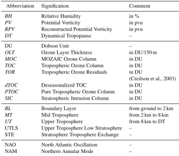
Table 1.List of used abbreviations.

Abbreviation Signification Comment

RH Relative Humidity in %

PV Potential Vorticity in pvu

RPV Reconstructed Potential Vorticity in pvu

DT Dynamical Tropopause –

DU Dobson Unit –

OLT Ozone Layer Thickness in DU/150 m

MOC MOZAIC Ozone Column in DU

TOC Tropospheric Ozone Column in DU TOR Tropospheric Ozone Residuals in DU

(Creilson et al., 2003)

dTOC Deseasonalized TOC in DU

PTOC Pure Tropospheric Ozone Column in DU SIC Stratospheric Intrusion Column in DU

BL Boundary Layer from ground to 2 km MT Mid Troposphere from 2 km to 8 km UT Upper Troposphere from 8 km to DT UTLS Upper Troposphere Low Stratosphere –

STE Stratosphere Troposphere Exchange –

NAO North Atlantic Oscillation – NAM Northern Annular Mode –

A subset of mid-latitudes MOZAIC sites, having high fre-quencies of observations and spread over the northern hemi-sphere, was selected. It comprised: Frankfurt (8.5 E, 50.0 N), with 6338 vertical profiles as two aircraft operate from this airport; Paris (2.6 E, 49.0 N), with 3308 vertical profiles; New York (74.2 W, 40.7 N), with 2631 vertical profiles; and the Japanese cluster of Tokyo (139.7 E, 35.6 N), Nagoya (136.8 E, 35.1 N) and Osaka (135.0 E, 34.0 N) with 1899 ver-tical profiles. The three Japanese cities visited by MOZAIC, all located on the Japanese Pacific coast and separated by at most 400 km, were treated as a single MOZAIC site rep-resenting the Japanese region, ensuring a suitable sampling frequency for this region. Profiles were defined as the part of the flight between ground level and the first pressure sta-bilized cruising level, usually up to about 300 hPa (200 hPa) with regard to the ascent (descent) profile. The ground tracks of the aircraft profiles formed a disk of about 400 km radius in Frankfurt and Paris, a quarter of a disk facing northeast in New York, and half a disk facing northwest over Japan. We consider aircraft profiles to be as valuable as balloon sound-ings for the computation of tropospheric ozone columns in spite of the fact that the atmospheric volumes delimited by the ground tracks of the aircraft vertical profiles are some-what larger than those of balloon soundings, and that the as-cent rates are greater for sounding balloons. These discrep-ancies have been evaluated by Thouret et al. (1998b).

(4)

J a n J u l J a n J u l J a n J u l J a n J u l J a n J u l J a n J u l J a n J u l J a n 9 5 9 6 9 7 9 8 9 9 0 0 0 1 0 2

J a n J u l J a n J u l J a n J u l J a n J u l J a n J u l J a n J u l J a n J u l J a n

9 5 9 6 9 7 9 8 9 9 0 0 0 1 0 2

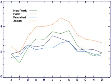
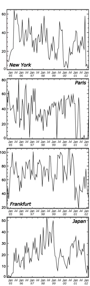
Fig. 1.Number of MOZAIC profiles per month over the 1994-2002

period for New York, Paris, Frankfurt and Japan stations.

2 profiles per month in September 1995, and some peri-ods with none in March 1998, December–January 2000 and May 2001–January 2002. An average of 30 profiles per month is reached in New York but with less than 10 profiles per month in December 1998–March 1999 and in January– February 2002. Japan has an average of 20 profiles per month but less than 5 profiles per month during August 1994–March 1995 and February 2002. Note that the mea-surement frequency for most of the ozone sounding stations of the northern hemisphere is weekly (WOUDC web site: http://www.nilu.no/niluweb/).

3 Definitions and methodology

3.1 Tropospheric ozone column

Within the MOZAIC data, it is not always possible to identify the height of the tropopause because the aircraft may not cross the tropopause during the ascent or de-scent. The criterion on the temperature lapse rate defined by WMO (1957) may be unverifiable because of the insuffi-cient vertical depth sampled by aircraft near the tropopause. Here, we use the definition of the dynamical tropopause (DT) given by Hoskins et al. (1985) which is a poten-tial vorticity surface corresponding to the value 2 pvu (with 1 pvu=10−6_m2_{K s}−1_kg−1_). _{Potential vorticity was} com-puted from 6-hourly ECMWF analyses with the T213 spec-tral truncation on the horizontal and with 31 vertical levels. Interpolation into the aircraft’ trajectories was performed us-ing a 3-D cubic Lagrange formulation for space and a simple linear formulation for time. In case of multiple intersections of the 2-pvu line with the vertical profile (see Fig. 2 for de-tails), the dynamical tropopause was defined to be where the highest part of the 2-pvu line crossed the vertical profile. We further arbitrarily consider three vertical layers in the depth of the troposphere. The layer from the dynamical tropopause to 8 km altitude will be referred to as the upper troposphere (UT), the 8–2 km altitude layer the mid troposphere (MT), and the 2–0 km altitude layer the boundary layer (BL).

To characterize the vertical distribution of ozone in the troposphere we chose to represent equivalent thicknesses of ozone in 150 m depth layers along the tropospheric column. In this way, tropospheric ozone columns (TOC) were cal-culated from the ground to the dynamical tropopause (see Fig. 2).TOC, expressed in Dobson Units (DU), is the equiv-alent thickness of ozone contained in the tropospheric col-umn compressed down to standard temperature and pressure (Andrews et al., 1987). The contribution to TOC of each 150 m depth layer of atmosphere is called the Ozone Layer Thickness (OLT), so thatTOCis the integration ofOLTfrom ground toDT, while the integration ofOLTfrom ground to the top of the MOZAIC vertical profile is calledMOC for MOZAIC Ozone Column. The detailed computation ofOLT

(5)

O L T

T O C

O L T

2 p v u

S I C

P T O C

T o p

0 m

M

O

Z

A

IC

v

e

rt

ic

a

l

p

ro

fi

le

M O C

( h = 1 50 m ) O L T

2 p v u D . T .

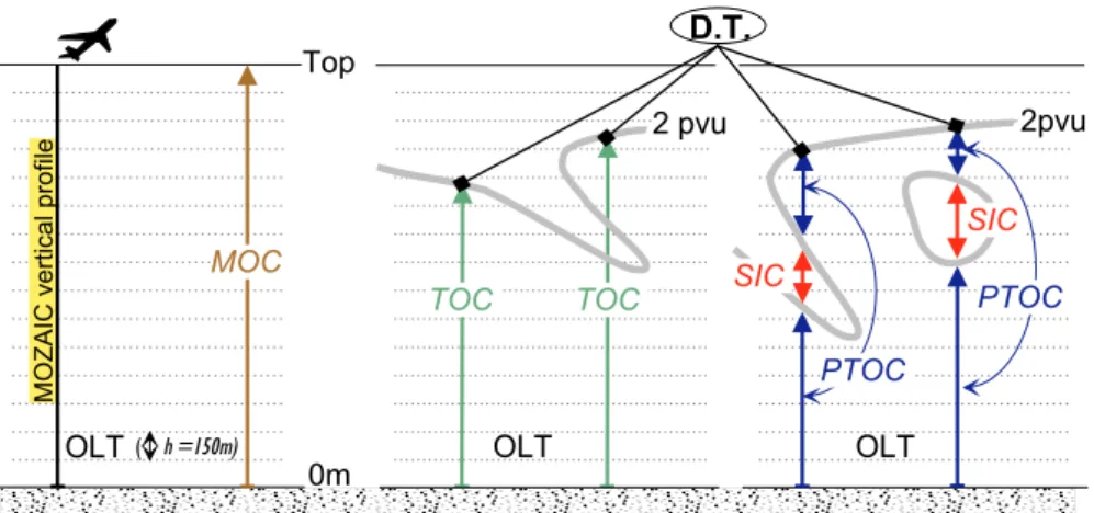
Fig. 2. Schematic definitions: Ozone Layer Thickness(OLT) is the equivalent amount of ozone expressed in DU (see Appendix) for a

150-m deep layer where full-resolution MOZAIC ozone data are averaged.MOZAIC Ozone Column(MOC) is the integrated ozone profile from the ground to the cruise altitude of the aircraft (noted Top).Tropospheric Ozone Column(TOC) is the integrated ozone profile from the ground to the Dynamical Tropopause (DT, black diamond). Coming down from the stratosphere,DTis the first intersection with the 2-pvu contour line. Stratospheric Intrusion Column(SIC) is the integrated ozone profile through layers that fulfil stratospheric-origin criteria below the dynamical tropopauseDT(see text for details). Pure Tropospheric Ozone Column(PTOC) is the difference between

TOCandSIC.

such ozone thicknesses is to help, on the one hand, the satel-lite remote sensing and the radiative transfer communities, mostly interested byTOCand, on the other, the regional air quality community, mostly interested in the volume mixing ratio, which can easily be derived fromOLT(see Eq. (6) in the Appendix). Although the vertical resolution of MOZAIC raw data is as good as a few tens of metres, we chose to computeOLT over a 150-m vertical depth to avoid useless computations of associatedPV profiles at very high vertical resolution with the ECMWF analyses.

Stratospheric intrusions into the troposphere occur dur-ing tropopause folddur-ing in narrow regions near upper-tropospheric fronts (Danielsen, 1968) and can be traced by characteristic features like high static stability, high ozone content, low water vapour content, and high potential vortic-ity. In the presence of a tropopause fold, e.g. when the 2 pvu contour folds below the dynamical tropopause level (see Fig. 2), ozone of stratospheric origin is included in theTOC

as we have defined it. TOCmay be dramatically increased with stratospheric-origin intrusions because ozone observa-tions across tropopause folds often show high ozone concen-trations. For instance, Danielsen et al. (1987) and Browell et al. (1987) reported mixing ratios of ozone in excess of 200 ppbv in a 2.0-km-deep tropopause fold observed with airborne lidar and in situ measurements in the upper tro-posphere. The contribution of stratospheric-origin ozone to

TOC assessed using Eq. (A6) (see Appendix) for a hypo-thetical tropopause fold of 1.5-km depth with a 150-ppbv homogeneous ozone mixing ratio at 400 hPa and−20◦C is about 10 DU (or equivalently 1 DU/150 m on the vertical), which may represent up to 50% (25%) of the monthly-mean

TOC observed at mid-latitudes during winter (summer) as

described in following sections. Stratosphere-troposphere exchange (STE) may therefore be a more or less important contributors to the tropospheric ozone budget according to whether intrusions are deep, transient or shallow when they penetrate into the troposphere (Wernli and Bourqui, 2002; Stohl et al., 2003). The identification of the stratospheric origin of air parcels with thermodynamical parameters may be achieved through Lagrangian approaches (Wernli and Davies, 1997; Stohl, 2001). Here, the Lagrangian parameter used, the Reconstructed Potential Vorticity (RPV), is thePV

value at the end of a 24-hour backward air parcel trajectory initialized at the location of the observation and computed with 6-hourly winds from ECMWF analyses. For backward trajectories the Lagrangian method uses a cubic polynomial interpolation of three-dimensional winds. A recent strato-spheric origin (≤24 h) is allocated to an air parcel if three criteria are met: RPV≥1.5 pvu, altitude>2000 m and ob-served relative humidity (RH)<50%. The criterion onRPV

is a compromise. It has to be less than that in order to take into account non-conservation effects in trajectories and the numerical diffusion by the parent model. The magnitude of

RPVhas to be large enough to avoid capturing tropospheric-origin air parcels withPVdiabatically enhanced in a region of strong latent heat release. The second criterion on the alti-tude prevents capture of air parcels with a relatively largePV

(6)

profile through layers that satisfy stratospheric-origin ozone criteria (RPV>1.5 pvu,z>2000 m, RH≤50%) below the dy-namical tropopause. The Pure Tropospheric Ozone Column (PTOC) is the difference betweenTOCandSIC.

In order to illustrate the computation of TOC, SIC and

PTOC quantities, four individual MOZAIC profiles over Frankfurt are illustrated in Fig. 3:

• The first vertical profile (Fig. 3a) presents typical sig-natures of the tropopause, like the change in the tem-perature lapse rate, the dryness, and the well defined vertical gradient of ozone mixing ratio. The dynami-cal tropopauseDT is given at 7850 m altitude with the

PV threshold which is correct with respect to the tem-perature lapse rate and acceptable with respect to the ozone mixing ratio as an universally accepted criterion on chemical tropopause is quite difficult to establish (Thouret et al., 1998a). In consequence, the rapid in-crease of the OLT profile from 0.6 to 0.8 DU/150 m just below the tropopause is counted as a contribu-tion to TOC, which is uncertain but has nevertheless a minor impact. TOC is about 21 DU and there is no contribution of stratospheric origin in it as theRPV pro-file never exceeds the 1.5 pvu threshold.

• The second vertical profile (Fig. 3b) also presents clear tropopause signatures in the observations, which is consistent with the dynamical tropopause given at 10 028 m. The RPV threshold method detects a typ-ical stratospheric-origin layer in the mid troposphere between 5812 m and 6679 m where ozone is anti-correlated with the relative humidity, and the temper-ature lapse rate is decreasing. In this layer, the ozone mixing ratio is higher than 100 ppbv, or equivalently,

OLT is larger than 0.8 DU/150 m. The contribution of

SICtoTOCis 5.93 DU, about 18% ofTOC.

• On the third vertical profile (Fig. 3c), the dynamical tropopause is defined and crossed at 9828 m. Data show a characteristic tropopause fold at around 4700 m alti-tude, with a 90 ppbv ozone peak, 10% minimum relative humidity and maximum OLT close to 0.8 DU/150 m. The case was studied by N´ed´elec et al. (2003) in a validation paper for ozone and carbon monoxide mea-surements from the MOZAIC programme. However, this tropopause fold is not detected by theRPV thresh-old method, and so does not contribute toSIC, though it does contribute to TOC. This shows that improve-ments of the Lagrangian approach would certainly be needed to capture all stratospheric intrusions. Below the tropopause there are some layers whereRPVexceeds its 1.5-pvu threshold, but these layers are considered to be of tropospheric origin because humidity is very high. • In the last example (Fig. 3d), the dynamical tropopause

is defined at 11 000 m and is not crossed by the aircraft,

which stops climbing at about 9 km altitude. The ver-tical profile ofOLT (in DU/150 m) has been filled up from 9128 m to the level of the dynamical tropopause with a method described in the next section. In the planetary boundary layer, ozone pollution is visible with a 80 ppbv maximum at 1000 m, OLT values exceed 1.2 DU/150 m and strongly contribute toTOC, which is close to 40 DU.

To summarise,TOCvalues of the previous MOZAIC pro-files are between 23 and 40 DU. The maximumOLT contri-bution toTOCcan be located in the boundary layer, the mid troposphere or the upper troposphere. A given ozone mix-ing ratio will obviously contribute more toTOCin the lower troposphere than at any other higher level in the troposphere, because of greater air density at lower altitudes (Eq. (A6) in the appendix).

3.2 Missing data in vertical profiles

Data may be missing from tropospheric profiles for two rea-sons. First, there are data gaps that are due to the operation of the MOZAIC ozone analyzer (internal calibration periods, resets, powercuts, etc.). Such data gaps take up one or sev-eral 150-m deep layers with a frequency that does not ex-ceed 5% of the data set used in this study. If data is miss-ing for just oneOLT (i.e., a 150-m deep layer; see Fig. 2) in a profile, then the missing value is computed using a lin-ear interpolation between data of the two nlin-earest layers in the same profile. If data for more than oneOLT are miss-ing (i.e. a gap exceedmiss-ing 150-m depth), each missmiss-ingOLT

value is replaced by its seasonal climatological value com-puted using the MOZAIC dataset (see Sect. 4.1). Second, there are the MOZAIC profiles that do not reach the dynami-cal tropopause. Here, our strategy is to fill up the unexplored atmospheric layers as high as possible by replacing missing

OLT values with their corresponding seasonal climatologi-cal values. If the dynamiclimatologi-cal tropopause for a given flight is situated above the top of the seasonal climatological profile (about 12 km altitude in practice for MOZAIC aircraft), the profile is filled up to the latter level. We decided not to fill up the unexplored remainder. The contribution toTOCof the unexplored remainder of the profile is all the more important since the tropopause is high. Nevertheless there is a balanc-ing effect due to the dependence ofOLT on pressure. The impacts of the filling-up process and unexplored remainders of profiles are evaluated and discussed below.

(7)

D . T . 1 0 / 0 2 / 2 0 0 2 T O C = 3 0 , 8 2 D U

S I C = 0 D U

D . T . 0 7 / 0 5 / 1 9 9 5 T O C = 3 9 , 8 0 D U S I C = 0 D U

D . T . 2 2 / 0 6 / 1 9 9 7 T O C = 3 2 , 7 3 D U S I C = 5 , 9 3 D U D . T .

1 5 / 0 7 / 2 0 0 0 T O C = 2 0 , 5 6 D U

S I C = 0 D U

a ) b )

c ) d )

Fig. 3. Individual MOZAIC vertical profiles (in km) over Frankfurt. Lower horizontal scale is for the ozone mixing ratio [in ppmv – red

dotted line],OLT [in DU – red solid line or red dashed line if the profile has been filled up to the altitude of the dynamical tropopause using the monthly-averageOLTprofile], relative humidity [×100% – blue line] and reconstructed potential vorticity [×10 pvu – black line]. The upper horizontal green scale is temperature [◦C– green line]. TOCis computed over a column from the ground to theDT[dark grey horizontal line]. A tropospheric layer contributes toSICif three criteria are met: altitude between 2 km and theDT, relative humidity lower than 50% and reconstructed potential vorticity exceeding 1.5 pvu (i.e. if the black line exits on the right of the shaded grey pattern).

Table 2.Statistics on MOZAIC vertical profiles available between August 1994 and February 2002 at the four stations: P is the total number

of available vertical profiles; P1 is the number of vertical profiles for which aircraft have crossed the dynamical tropopause; P2 is the number of vertical profiles that have been filled up to the dynamical tropopause with the corresponding part of the seasonal-average tropospheric

OLTprofile (see Fig. 6); P3 is the number of vertical profiles unavailable for the study because PV data are missing; P4 is the number of vertical profiles for which the aircraft did not cross the tropopause and for which the tropopause of the day is above the highest altitude level defined by the seasonal-average troposphericOLTprofile. Values in brackets are corresponding percentages.

Station P P1 P2 P3 P4

Frankfurt 6338 2813 (44.4) 3015 (47.6) 100 (1.6) 410 (6.5) Paris 3308 1307 (39.5) 1662 (50.2) 45 (1.4) 294 (8.9) New York 2631 881 (33.5) 1006 (38.2) 25 (1.0) 719 (27.3) Japan 1899 360 (19.0) 481 (25.3) 23 (1.2) 1035 (54.5)

Japan (column P2). Some vertical profiles are still uncom-pleted after this step because thePV profiles are not avail-able in the data base; this occurs for less than 2% of the pro-files whatever the site (column P3). Finally, there are other uncompleted profiles because the tropopause of the day is higher than the maximum altitude of the seasonal climato-logical profile. The proportion of profiles affected ranges from 6.5% over Frankfurt to 54.5% over Japan (column P4). The statistics of the Japanese profiles are very different from

(8)

F r a n k f u r t

P a r i s

J a p a n

N e w - Y o r k

Fig. 4.Monthly-mean pressures of the dynamical tropopauseDT(in hPa) deduced with aPVthreshold (2 pvu) on ECMWF analyses at the

four stations: blue lines showDTsampled at the frequency of MOZAIC aircraft, black lines showDTsampled at the frequency of MOZAIC profiles that cross the tropopause (column P1 in Table 2), and red lines showDTwith the sampling frequency of MOZAIC profiles that cross the tropopause or that have been filled up to it (columns P1, P2 and P4 in Table 2, see text for details).

N e w - Y o r k P a r i s F r a n k f u r t J a p a n

Fig. 5.Monthly-mean contribution to the Tropospheric Ozone

Col-umn (DU) by the filling-up process applied on MOZAIC vertical profiles in columns P2 and P4 of Table 2.

filling-up process weights the assessment of the short-term trend ofTOCwith the contribution of a fixed seasonal value, and there is an underestimation ofTOCfor P4 profiles. These effects, which may become important in New York and Japan during summertime when the tropopause is the highest, are assessed below. Note that a further extension of the present work would be to consider known ozone climatologies (e.g., Logan, 1999) in order to fill in any missing vertical ozone data over MOZAIC sites.

Monthly mean pressure of the dynamical tropopause for the four MOZAIC sites is shown on Fig. 4. Blue lines are results in pressure of the tropopause detection method with thePV threshold on ECMWF analyses at the sampling fre-quency of MOZAIC flights (Column P in Table 2). A marked low (high) tropopause is visible in winter (summer) over New York and over Japan, whereas the seasonal variations of tropopause pressure over Frankfurt and Paris are rather small. Differences are mainly due to the positions of the sites

(9)

investigation of short-term trends by introducing a compo-nent that is time-independent in the dataset.

4 Climatological analysis

4.1 Vertical profiles

Seasonal climatological vertical profiles ofOLT are plotted on Fig. 6. The vertical gradient of OLT is positive in the boundary layer whatever the season and the site, and be-comes negative in the free troposphere. Then, a difference can be seen according to whether the seasonal-mean is com-puted with all profiles (thin lines) or with sections of the pro-files below the dynamical tropopause (thick lines).

With all profiles, the large stratospheric ozone concentra-tions make the vertical gradient of OLT return to positive values in the upper part of the profile (Fig. 6, thin lines). The range of altitudes where the vertical gradient of OLT

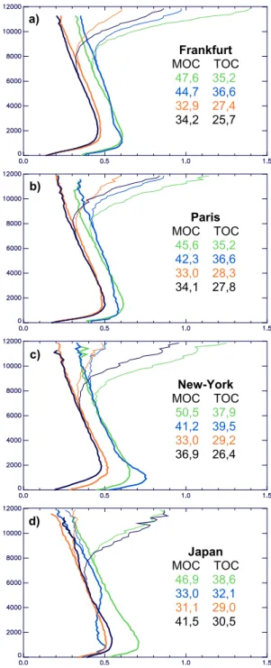
changes its sign is close to the seasonal-mean tropopause, i.e. between 8 and 10 km on every station and for every sea-son except i) over New York in winter and spring, and Japan in winter, where the changes occur slightly below 8 km, ii) over New York in summer, and Japan in summer and au-tumn, where the change occurs above 10 km. A noticeable feature is thatOLT, in this region of 8–10 km altitude, has values smaller than in the planetary boundary layer. In the context of the links between ozone trends in the UTLS region and radiative forcing, the latter feature is important because the contribution of a perturbation on the ozone vertical pro-file to the change in surface temperature is maximum in the UTLS region (Forster and Shine, 1997). Because the ceiling altitudes of MOZAIC aircraft are nearly always below the tropopause over Japan in summer and autumn, the positive vertical gradient ofOLTin the lower stratosphere is not de-fined on the seasonal time scale. In the lower stratosphere, maximumOLT values are observed during spring and range from 0.9 DU/150 m over Japan to 1.4 DU/150 m in Frankfurt. MinimumOLT values of about 0.5 DU/150 m are observed during autumn. Seasonal-mean values ofMOC, i.e. vertical integrals of thin lines, range from 31 to 50 DU and go through a maximum in spring at each MOZAIC station.

With all sections of the profiles below the dynamical tropopause (Fig. 6, thick lines), seasonal climatological pro-files are such that the negative vertical gradient ofOLT ex-tends up to the MOZAIC aircraft ceiling in the uppermost troposphere. Seasonal-mean values ofTOC, i.e. vertical in-tegrals of thick lines shown in Fig. 6, range from 26 to 39 DU and go through a maximum in summer at each MOZAIC sta-tion except Japan. Very well defined maxima of OLT are observed in the planetary boundary layer. New York has the highest ozone-polluted boundary layer in summer with a maximum of 0.75 DU/150 m. An exception occurs for Japan where maritime-origin ozone-poor air masses of the summer-monsoon season are associated with lowOLT values up to

F r a n k f u r t M O C T O C

4 7 , 6 3 5 , 2 4 4 , 7 3 6 , 6 3 2 , 9 2 7 , 4

3 4 , 2 2 5 , 7

P a r i s M O C T O C

4 5 , 6 3 5 , 2 4 2 , 3 3 6 , 6 3 3 , 0 2 8 , 3

3 4 , 1 2 7 , 8

N e w - Y o r k M O C T O C

5 0 , 5 3 7 , 9 4 1 , 2 3 9 , 5 3 3 , 0 2 9 , 2

3 6 , 9 2 6 , 4

J a p a n M O C T O C

4 6 , 9 3 8 , 6 3 3 , 0 3 2 , 1 3 1 , 1 2 9 , 0

4 1 , 5 3 0 , 5 a )

b )

c )

d )

Fig. 6. Seasonal climatological vertical profiles (in m) of Ozone

Layer Thickness (OLT, in DU/150 m) for Frankfurt, Paris, New York and Japan. (Thin lines): no distinction is made with regard to the altitude of the dynamical tropopause. Vertical integrals are the seasonal climatologicalMOC(DU). (Thick lines): made with sections of the profiles below the dynamical tropopause. Vertical integrals are the seasonal climatologicalTOC(DU). Colors: green for spring, blue for summer, orange for autumn and black for winter.

(10)

S p r i n g :

M a r

A p r

M a y

S u m m e r :

J u n

J u l

A u g

F r a n k f u r t

F a l l :

S e p

O c t

N o v

W i n t e r :

D e c

J a n

F e b

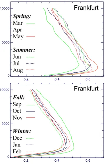
Fig. 7. Monthly-mean tropospheric profiles (in m) of OLT

(DU/150 m) over Frankfurt.

profiles. This classification also shows up on a monthly ba-sis as seen, for instance, for Frankfurt (see Fig. 7). March and September appear to be transitional months between the two classes. Synthetic ozone profiles can be easily built from these averaged data for initialization purposes in chemistry transport models and retrieval techniques for satellite prod-ucts.

4.2 Seasonal cycle

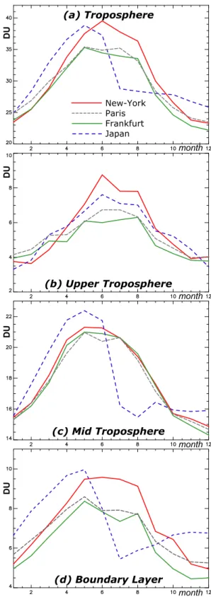
The seasonal cycle of monthly-mean TOC over MOZAIC sites is presented in Fig. 8a. Paris and Frankfurt show a very similar seasonal cycle with a broad maximum of about 34 DU from April to August and a minimum of about 22 DU in December. The seasonal cycle over New York is similar to European cycles except for its larger range with a broad spring-summer maximum that peaks at 39 DU in June. It is interesting to note the rapid springtime increase at the three stations and then a dropping off during the late summer. The rapid springtime increase is consistent with photochemical

ozone production after ozone precursors have accumulated in the troposphere in winter and when insolation increases. The contribution of stratosphere-troposphere exchange to this cy-cle is discussed in the following section. Over Japan, the sea-sonal cycle is quite different. The earlier springtime increase is consistent with a latitudinal effect (earlier springtime sun) as Japanese stations are the southernmost stations considered here. Winter and spring values are 2–3 DU larger than those at other sites. The cycle goes through a 38 DU maximum in May, then abruptly falls to 28 DU during the summer-monsoon season (July) and slowly decreases to 25 DU in De-cember.

The fourUTseasonal cycles (Fig. 8b) are all in phase; they display a maximum in late spring (except Frankfurt) and a secondary maximum (except Paris) in late summer. The am-plitude is larger for New York and for Japan, in agreement with the summertime elevated tropopause there. The phas-ing of all fourUTcycles suggests that the summer monsoon over Japan does not influence the upper-tropospheric ozone budget.

Mid-tropospheric contributions toTOC(Fig. 8c) are pre-dominant (≈60% ofTOC). Interestingly, the two European seasonal cycles are almost identical to the one for New York. The peak is in May-June and the minimum in December. It is likely that the similarity of these three mid-tropospheric cy-cles has something to do with the homogenization of the dis-tributions of trace gases that have a sufficient lifetime (a few weeks), like ozone, by the large-scale circulation. The lat-itudinal and the summer-monsoon effects that influence the Japanese seasonal cycle are clearly visible in the mid tropo-sphere.

Boundary layer contributions (Fig. 8d) represent roughly a 25% contribution to TOC. These contributions are 10% higher in New York compared to Frankfurt and Paris during spring and summer, and are 10% higher in Japan compared to New York, Frankfurt and Paris during autumn and early spring. Local and remote anthropogenic emissions as well as biomass burning over upstream regions of Asia may be responsible for larger low- and mid-tropospheric contribu-tions toTOCover Japan throughout the year except during the summer-monsoon season.

(11)

come from the missing contribution in the upper troposphere when tropopause-crossings by MOZAIC aircraft diminish. The summertime underestimations of TOC are less than 1 DU in Frankfurt and 5 DU in New York.

4.3 Stratospheric Intrusion Column

The purpose here is to test the validity of the Lagrangian approach used to detect stratospheric-origin air parcels (see Sect. 3.1), and to evaluate the contribution of the stratospheric-origin ozone, i.e. the Stratospheric Intrusion ColumnSIC, to the Tropospheric Ozone ColumnTOC. Over Japan, there is a large seasonal variation in the frequency of flights affected by STE (i.e.,SIC>0), from 69% in January down to 15% in August (not shown). Such a large frequency range may be explained by favourable wintertime dynamics for STE in the region of the subtropical jet (Sprenger et al., 2003) and by unfavourable summertime monsoon dynamics. Over Paris, Frankfurt and New York and whatever the season, about one third of the vertical profiles contain signatures of stratosphere-troposphere exchange (not shown). The quasi-absence of seasonal variation of STE frequency over New York, Paris and Frankfurt stations is an indication that the criterion used here to computeSICaccumulates transient and deep events. According to Lagrangian studies exploring the sensitivity of the residence time criterion of air parcels (e.g. Wernli and Bourqui, 2002; James et al., 2003), transient and deep events respectively lead to weak and strong seasonal cy-cles of the zonally integrated cross-tropopause mass-fluxes. Tropospheric depths of tropopause folds are quite variable. For instance, Danielsen et al. (1987) observed a depth that decreased from 2 to 0.6 km as the folds descended from 6 to 2 km altitude. In accordance with the latter study, the average depth of stratospheric-origin layers assessed here is 750±150 m. Monthly-mean concentrations of ozone ob-served in stratospheric intrusions are shown on Fig. 9a for the upper troposphere and the mid troposphere. Mean con-centrations in the upper troposphere are higher than in the mid troposphere for every month and every station (except for July over New York, October over Paris and March over Japan, where opposite differences not exceeding 15 ppbv come from irregularities in the sampling frequency). During the monsoon season (August) over Japan, there is no strato-spheric influence detected in the mid troposphere. An up-per tropospheric maximum forms in May–June, with about 150 ppbv over New York and Japan, and 110 ppbv over Paris and Frankfurt. An upper tropospheric minimum ranges from 70 to 90 ppbv during winter over the four stations. Some observed values exceed 250–300 ppbv which indubitably in-dicates stratospheric origin. For ozone layer thickness asso-ciated with stratospheric-origin air, Fig. 9b shows the same general behaviour as for concentrations, except that this time mid-tropospheric values are always slightly larger than upper-tropospheric ones (except Japan in July) in agreement with the difference of air density. Note that springtimeOLT

( a ) T r o p o s p h e r e

( b ) U p p e r T r o p o s p h e r e

( c ) M i d T r o p o s p h e r e

( d ) B o u n d a r y L a y e r

N e w - Y o r k P a r i s F r a n k f u r t J a p a n

m o n t h

D

U

m o n t h

D

U

m o n t h

D

U

m o n t h

D

U

Fig. 8. Monthly-mean TOC seasonal cycle: (a) Total

(12)

New York

Japan Paris

Frankfurt

UT MT

New York

Japan Paris

Frankfurt

UT MT

Fig. 9. (Top) Monthly-mean ozone concentration (ppbv) of 150 m-deep layers affected by stratosphere-troposphere exchange for the mid

troposphere (red line) and for the upper troposphere (black line) over the four MOZAIC stations. (Bottom) Same as the top panel but for the ozone layer thickness (DU/150 m). In both panels the red (black) points correspond to individual observations in the mid troposphere (upper troposphere).

affected by stratospheric intrusions are about 0.6 DU/150 m, which is close to the maximum of meanOLTvalues observed in the polluted planetary boundary layer (see Fig. 6). If iso-lated maximum values are considered, both in mid- and in upper troposphere, they exceed 1.0 DU/150 m which is com-parable to lower-stratospheric values.

(13)

of the troposphere at any one time has been in the strato-sphere within the preceding year. Roelofs and Lelieveld’s (1997) model-derived figure of 40% pertains to the total con-tribution of ozone of stratospheric origin to the tropospheric ozone, whereas our estimate only includes recently added stratospheric air that has not had a chance to mix and be di-luted by tropospheric air. Taking into account that several factors reduce the capture of stratospheric intrusions in our Lagrangian method (see Sects. 3.1 and 3.2), this is a strong result that confirms that the important role of stratosphere-troposphere exchange in the tropospheric ozone budget can be further investigated with the MOZAIC dataset. Our re-sults lay the foundations for further observation-based stud-ies where improvements in the retrieval of SIC from the combination of MOZAIC data and a Lagrangian approach may include i) the computation of longer backward trajec-tories (>5 days) to exploit the sensitivity to the residence time criterion to distinguish between transient and deep ex-changes, ii) advection with 3-hourly wind fields (analysis al-ternating with 3-hour forecasts) to reduce interpolation errors due to the linear assumption on temporal changes, iii) the use of ERA40 re-analyses at ECMWF, which provide bet-ter quality fields than operational analyses in the 1990s at the beginning of MOZAIC and allow inter-annual variabil-ity in stratosphere-troposphere exchange to be inferred, iv) the comparison with a particle dispersion model (Stohl et al., 2000) where effects of turbulent mixing and deep convec-tion are parameterized, v) the use of MOZAIC raw data (bet-ter vertical resolution with 4 s time resolution measurements, ≃20–30 m vertical resolution), vi) other MOZAIC stations to complete the northern mid-latitudes study (Washington D.C., Chicago, Vienna, ...), vii) further verification with the MOZAIC CO measurements. However, beyond the rough assessment ofSIC, we do not think that the precision of the present results allows inter-annual variability and short-term trends ofTOCandPTOC to be investigated separately. In consequence, the following section concentrates on the short-term trends and inter-annual variability ofTOC.

5 Short-term trends and interannual variability

The present MOZAIC 7-year dataset allows a limited in-vestigation of the inter-annual variability of the tropospheric ozone column and an assessment of the short-term trends. First, time series of monthly-meanTOC are considered in Sect. 5.1. Then, in Sect. 5.2, the inter-annual variability of

TOCin association with positive and negative phases of the North Atlantic Oscillation is discussed.

5.1 Short-term trends

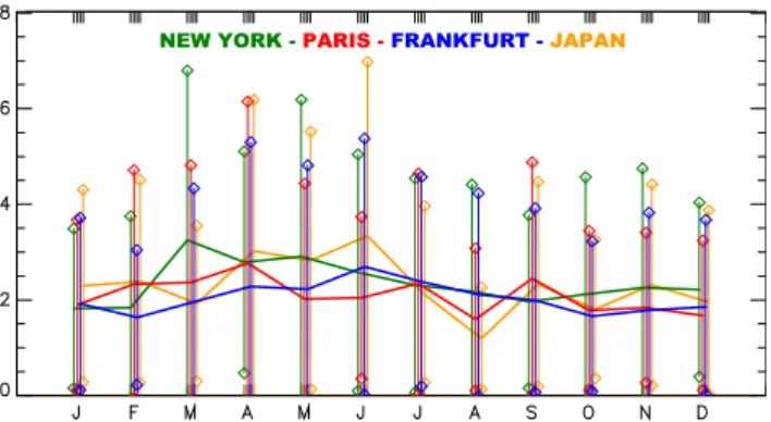
The time series of the monthly meanTOCfrom August 1994 to February 2002 at the four MOZAIC sites are shown on Fig. 11. Seasonal cycles go through a minimum in winter

N E W Y O R K - P A R I S - F R A N K F U R T - J A P A N

Fig. 10. Monthly-mean values of the Stratospheric Intrusion

Col-umn (SIC in DU), i.e. the integrated ozone profile through tro-pospheric layers that meet stratospheric-origin criteria. Vertical bars represent the standard deviations (DU). Colour code: blue for Frankfurt, red for Paris, green for New York, and orange for Japan.

and a maximum in summer, except for Japan where the max-imum occurs during the spring because of the arrival of the monsoon in summer. The New York and Japan stations have the largest amplitude, roughly from 20 DU to 44 DU. The Paris and Frankfurt stations have a lower amplitude, roughly from 20 DU to 36 DU, and quite similar time series (except for differences due to better sampling over Frankfurt). Some noticeable and common features are i) highTOC values in summer 1998 over New York, Paris and Frankfurt, ii) high

TOCvalues in summer 1999 over New York and Japan, iii) highest wintertimeTOCin 1999 over all four stations, rang-ing from 24 to 26 DU, iv) continuous increase of wintertime

TOCfrom 1996 to 1999 at New York, Paris and Frankfurt. Visual inspection of seasonal cycles in Fig. 11 gives the im-pression of a positive trend. This was confirmed by a statis-tical linear trend analysis over the 1995–2001 period, which shows a linear increase ranging from 0.7%/year in Frankfurt to 1.1%/year in New York. Note that incomplete seasonal cy-cles of 1994 and 2002 were discarded. The short-term trend over Paris (1.6%/year) is derived over the 1995–1999 period as important data gaps in 2000 and 2001 prevent complete assessment of the seasonal cycle for these years.

(14)

New York

TOC = 30.3 DU

+ 1.1 % /year

TOC in DU

1995 1996 1997 1998 1999 2000 2001

Paris

TOC = 29.7 DU

+ 1.6 % /year

Frankfurt

TOC = 28.5 DU

+ 0.7 % /year

Japan

TOC = 30.2 DU

+ 0.8 % /year

Fig. 11.Time series of monthly mean Tropospheric Ozone ColumnTOC(DU, red solid lines) from August 1994 to February 2002 for the

4 MOZAIC stations. Indications on the right summarize the annual-meanTOC(DU) and short-term trends (%/year) over the 1995–2001 period, or over the reduced 1995–1999 period for Paris.

relation to the linear increase, a wintertime bump or anomaly clearly appears in 1997 and 1998 at all four stations. Such an anomaly is more or less well defined from autumn 1997 to summer 1999 at all stations.

Table 3 sums up the annual-mean and seasonal-mean of

TOC(DU) and the related trends (%/year). It also details the contribution toTOC of the boundary layer, the mid tropo-sphere and the upper tropotropo-sphere. Noticeable wintertime fea-tures in New York, Paris and Frankfurt are the strong trends exceeding 3%/year in the boundary layer and 1.7%/year in

(15)

S E A S O N A L T O C : S P R I N G ( M - A - M ) S U M M E R ( J - J - A ) F A L L ( S - O - N ) W I N T E R ( D - J - F ) Y E A R L Y T O C : T O C I A V :

N e w Y o r k 3 7 . 8 D U - 0 . 0 % / y e a r

3 3 . 4 D U + 1 . 5 % / y e a r

2 6 . 8 D U + 0 . 8 % / y e a r

2 4 . 0 D U + 1 . 9 % / y e a r

P a r i s 3 3 . 9 D U + 0 . 1 % / y e a r

3 2 . 5 D U + 0 . 5 % / y e a r

2 6 . 2 D U + 0 . 4 % / y e a r

2 5 . 3 D U + 2 . 0 % / y e a r

2 3 . 9 D U + 2 . 0 % / y e a r F r a n k f u r t

3 4 . 0 D U - 0 . 0 % / y e a r

3 2 . 0 D U + 1 . 3 % / y e a r

2 5 . 1 D U + 0 . 3 % / y e a r

J a p a n

2 6 . 4 D U + 1 . 0 % / y e a r

3 6 . 1 D U + 0 . 9 % / y e a r

2 7 . 5 D U + 0 . 8 % / y e a r

3 1 . 5 D U + 0 . 1 % / y e a r

Fig. 12.Yearly seasonal-means for Tropospheric Ozone Column (DU) from 1994 to 2001 for the 4 MOZAIC stations (solid lines, green for

spring, blue for summer, orange for autumn, black for winter). Dotted lines are the linear regression fits. Averaged seasonal-meanTOC(DU) and seasonal linear increase (%/year) computed for the 1995-2001 period are displayed on the left part of each plot.

Table 3. Annual and seasonal mean ofTOC(DU), and corresponding short-term trends (%/year) for the entire troposphere and for the

boundary layer (BL, 0–2 km altitude), mid troposphere (MT, 2–8 km altitude) and upper troposphere (UT, 8 km altitude to the dynamical tropopauseDT) over New York, Paris, Frankfurt and Japan.

Annual Spring Summer Fall Winter

DU %/year DU %/year DU %/year DU %/year DU %/year

TOC 30.3 1.1 33.4 1.5 37.8 0.0 26.8 0.8 24.0 1.9

New York TOC in BL 7.2 0.4 8.3 1.2 9.4 −1.2 6.2 1.2 5.4 3.9

2631 profiles TOC in MT 17.9 1.2 20.0 1.2 20.3 0.6 16.2 1.0 15.6 2.0

TOC in UT 5.5 1.3 5.7 1.6 8.1 0.1 4.8 −0.1 3.8 −0.7

TOC 29.5 0.9 32.5 0.5 34.3 0.2 26.2 0.4 25.3 2.0

Paris TOC in BL 6.8 0.9 7.9 0.3 7.8 0.3 5.8 0.6 5.8 3.1

TOC in UT 5.2 −0.1 5.5 −0.9 6.6 −0.4 4.6 −0.2 4.2 1.9

TOC 28.5 0.7 32.0 1.3 34.0 0.0 25.1 0.3 23.9 2.0

Frankfurt TOC in BL 6.2 0.3 7.5 0.5 7.7 −0.2 5.1 0.7 5.0 3.3

TOC in UT 4.9 0.8 5.3 1.2 6.2 0.2 4.2 0.0 4.0 1.7

TOC 30.2 0.8 36.1 0.9 31.5 0.1 27.5 0.8 26.4 1.0

Japan TOC in BL 7.4 −0.1 9.5 0.5 6.4 0.1 6.6 0.3 7.1 0.3

(16)

The results presented above agree well with other results found in analyses of long-term series of ozone and cited in the introduction. In particular, trends in the short-term rang-ing from 0.7 to 1.1%/year forTOC(New York, Frankfurt and Japan) are in good agreement with the longer-term positive trend of 0.7 to 1.4%/year over Central Europe reported by Weiss et al. (2001) with ozonesonde data. Further compar-isons of our results with those by Naja et al. (2003) are of interest. Using the residence times of air masses over Cen-tral Europe (computed from 10-day backward trajectories), Naja et al. (2003) analyze the Hohenpeissenberg and Pay-erne ozonesonde dataset and classify ozone observations as-sociated with central European residence times of 4–6 days as “photochemically aged” ozone. It is shown that, in the range of 1–6 days of residence time, on average and in sum-mer, the mixing ratio of the latter class of ozone increases at a rate of 2 ppbv per day of residence time. Then, by ex-trapolation to zero days of residence time (using a statistical regression model), the authors build a “background” ozone value which is supposed to represent Atlantic air masses not influenced by European emissions. Although there is no con-sideration of residence time of air masses over continents in our study, three points of agreement with the findings of Naja et al. (2003) may be found. First, Naja et al. (2003) show that the “photochemically aged” ozone is maximum in sum-mer, minimum in winter, and has been experiencing a sub-stantial decrease in the planetary boundary layer in summer-time since the 1990s in agreement with temporal variations of Central European NOxemissions. This is in good agree-ment with the negative trends ofTOCin the boundary layer in summertime for New York and Frankfurt reported here (see Table 3). Note that further extension of this work would need to consider the top of the boundary layer, the impor-tance of the diurnal cycle of the boundary layer and of the airport position relative to its associated urban area, which is out of the scope of the present paper. Second, Naja et al. (2003) show positive trends of ozone in “background’ and in “photochemically aged” air in winter. It is in good agree-ment with the consistent positive trends found in wintertime and for the full tropospheric column at the four MOZAIC stations (except for New York in the upper troposphere, see Table 3). Third, Naja et al. (2003) show that “background” ozone in the planetary boundary layer and in the free tropo-sphere has a broad maximum extending from late spring to summer, has a minimum in winter and is experiencing in-creasing influences of emissions from North America and Eastern Asia. The importance of background pollution and intercontinental transport has been suggested by many other authors (e.g. Berntsen et al., 1996; Jacob et al., 1999; Wild and Akimoto, 2001). The common behaviour of yearly sea-sonal meanTOCat the four MOZAIC stations (see Fig. 12) is strongly suggestive of a consistent influence of background pollution transported by the general circulation. Therefore, station-to-station comparisons and links with the variations of the general circulations patterns are now discussed.

5.2 General circulation patterns

The North Atlantic Oscillation (NAO) is one of the most dominant and regular patterns of atmospheric circulation variability from the United-States to Siberia and from the Arctic to subtropical Atlantic (Wallace and Gutzler, 1981; Barnston and Livezey, 1987). It takes the form of a dipole anomaly in the surface pressure field between Iceland and the Azores. Here, we use the NAO index defined as the difference of normalized sea level pressure between Lisbon, Portugal and Reykjavik, Island (Hurrell, 1995). At the hemi-spheric scale, geopotential anomalies ranging from the sur-face to the stratosphere are dominated by a mode of vari-ability known as the Northern Annular Mode (NAM) also called the Arctic Oscillation (Baldwin and Dunkerton, 1999). In order to incorporate the Japanese MOZAIC stations in our investigation we also considered NAM, which has a broader centre of action than NAO in the northern hemi-sphere. We used monthly-mean mid-tropospheric (500 hPa) NAM indices provided by M. Baldwin (http://www.nwra. com/resumes/Baldwin/nam.html). Positive trends of NAO and AO in recent decades suggest that circulation changes may contribute to the observed winter trends of total (strato-spheric and tropo(strato-spheric) ozone (Appenzeller et al., 2000; Thomson et al., 2000; Br¨onniman et al., 2000).

(17)

1 9 9 5 1 9 9 6

2 0 0 0

1 9 9 7 2 0 0 1

1 9 9 9

1 9 9 8

F R A N K F U R T

N E W -y O R K

c o l o u r = N A O

1 9 9 5 1 9 9 6

2 0 0 0

1 9 9 7

2 0 0 1

1 9 9 9

1 9 9 8

F R A N K F U R T

J

A

P

A

N

c o l o u r = N A M

1 9 9 5

1 9 9 6 2 0 0 0

1 9 9 7

2 0 0 1

1 9 9 9

1 9 9 8

N E W - Y O R K

J

A

P

A

N

c o l o u r = N A M

- N A O - N A M

-N e w - Y o r k - F r a n k f u r t - J a p a n

( a )

( b )

( d )

( c )

T O C i n D U

T O C i n D U T O C i n D U

T O C i n D U T O C i n D U T O C i n D U

N A M

+ 0 . 2

+ 0 . 1

0

- 0 . 1

- 0 . 2

- 0 . 3

< - 0 . 4

N A O

+ 0 . 5

+ 0 . 3

+ 0 . 1

- 0 . 1

- 0 . 3

- 0 . 5

< - 0 . 7

Fig. 13. (a): Time series from 1995 to 2001 of monthlyTOCanomalies (DU) in New York (green line), Frankfurt (blue line) and Japan

(red line) and of indices for NAO (black lines) and NAM (grey line).(b): MonthlyTOCanomalies (DU) in New York versus monthlyTOC

anomalies (DU) in Frankfurt. Months are symbolized by squares. A coloured line encircles months of one year. The colour of each square is coded with the NAO index scaled regularly in 7 classes between−0.7 and 0.5 as given on the right part of the figure. The black line indicates the linear regression that best fits inter-stationTOCanomalies (see Table 4).(c): as for (b) but for Japan versus Frankfurt and for the NAM index at 500 hPa. The colour of each square is coded with the NAM index scaled regularly in 7 classes between−0.4 and 0.2 as given on the right part of the figure.(d): as for (c) but for Japan versus New York.

that the transport over the Atlantic occurs not only in the free troposphere but also in the boundary layer.

NAO and NAM display considerable monthly and inter-annual variability (Hurrell, 1995). Their effects reach the highest point during wintertime but have been observed at all seasons. In the construction of time series of monthlyTOC

anomalies (Fig. 13a), each monthlyTOCis deseasonalized by subtracting its annual-mean value (Fig. 8). To lessen the monthly variability and to capture the extra-seasonal signal shown on Fig. 12, we smooth the time series with a run-ning window of±6 months. The good overall coherence of all parameters over four major periods is striking. The period 1995–1996 shows negativeTOCanomalies and neg-ative NAO/NAM indices. It is followed by a transition year in 1997. Then comes the 1998–1999 period with positive

TOC anomalies and positive NAO/NAM indices. Finally, there is the last period 2000–2001 during which parameters show less mutual coherence and a gradual transition to neg-ative values. Note that the most important information of Fig. 13a, i.e. the transition from a period of negativeTOC

anomalies to a period of positive anomalies, is only brought about by the contribution of the mid troposphere (not shown). Monthly time series of the contributions of the boundary layer and the upper troposphere do not show up this tran-sition, which suggests that the mid-tropospheric long-range

transport of ozone may be the dominant process. Figure 13b shows the plot of monthlyTOCanomalies in Frankfurt ver-sus in New York, symbols are colour-coded with NAO in-dices. There is a strong relationship betweenTOCanomalies of the two stations, which is confirmed by a very high corre-lation factor (r=0.97, see Table 4). This correlation factor is even higher than the positive correlation factor betweenTOC

(18)

Table 4. Parameters deduced from linear regression fit be-tweenTOCanomalies (notedT OC′) themselves and betweenTOC

anomalies and NAO or NAM indices over Frankfurt, New York and Japan (see Fig. 13). a and b are parameters of the linear regression fit, r is the correlation factor andσthe standard deviation.

T OC′/T OC′ a b r σ

Frankfurt–New York 1.51 0.08 0.97 0.31 Frankfurt–Japan 1.17 0.11 0.89 0.47 New York–Japan 0.73 0.07 0.89 0.48

T OC′/N AO a b r σ

Frankfurt 0.41 −0.26 0.66 0.38

New York 0.26 −0.28 0.66 0.38

T OC′/N AM a b r σ

Japan 0.05 −0.16 0.33 0.16

warmest winter since 1895. Global temperatures in 1998 were the warmest in the past 119 years and the previous record was set in 1997 (see the Annual Review on climate of 1998 on the NOOA web site2). These warmer conditions may have globally favoured the photochemical production of ozone in the troposphere, which, coupled with the transition towards positive NAO/NAM indices, may have also favoured the long-range transport of higher background ozone concen-trations. Whether or not the transition of negative to positive NAO phases in this period could be a response to anthro-pogenic forcing, as suggested by some model scenario ex-periments in which enhanced greenhouse gas concentrations are prescribed (Ulbrich and Christoph, 1999), or may be bet-ter understood in bet-terms of an intrinsic dynamical property of the North Atlantic atmosphere (Cassou et al., 2004) is out-side the scope of the present study.

6 Conclusions

We have investigated climatological and inter-annual vari-ability aspects of ozone vertical profiles obtained at four sta-tions, Frankfurt (Germany), Paris (France), New York (USA) and the cluster of Tokyo, Nagoya and Osaka (Japan), by com-mercial aircraft participating in the MOZAIC programme from August 1994 to February 2002. This database of several thousands of vertical profiles constitutes one of the most in-teresting datasets currently available with regard to research issues on the tropospheric ozone budget and recent short-term trends. The study focuses on the analysis of two vertical integrated quantities in the troposphere, i.e. the Tropospheric Ozone Column (TOC), which is the vertical integration of ozone from the ground to the dynamical tropopause, and the 2_{http://lwf.ncdc.noaa.gov/oa/climate/research/1998/ann/ann98.} html)

Stratospheric Intrusion Column (SIC), which is the vertical integration of stratospheric-origin ozone throughout the tro-posphere. Commercial aircraft generally fly in the altitude range 9–12 km, so ascent and descent profiles at airports do not systematically include the tropopause region. Taking into account the interest of working on a large number of vertical profiles and the necessity of having profiles in the full depth of the troposphere (to compute the integrated quantities), our strategy has been to fill up unexplored parts of the vertical profiles as far as possible with seasonal climatological pro-files. This avoids biasing the results towards meteorologi-cal situations for which the tropopause is systematimeteorologi-cally low. The impact that the filling-up process may have on the inves-tigation of short-term trends by introducing a component that is time-independent in the dataset is limited to the summer-time uppermost troposphere in New York and Japan.

The climatological analysis shows that theTOCseasonal cycle ranges from a wintertime minimum of about 22–25 DU at all four stations to a spring-summer maximum of about 35 DU in Frankfurt and Paris, and 38 DU in New York. Over Japan, the maximum occurs in spring because of the earlier springtime sun, then the invasion of monsoon air masses in the boundary layer and in the mid troposphere steeply di-minishes the summertime TOC. Boundary layer contribu-tions toTOCare 10% higher in New York than in Frankfurt and Paris during spring and summer, and are 10% higher in Japan than in New York, Frankfurt and Paris during autumn and early spring. Local and remote anthropogenic emissions and biomass burning over upstream regions of Asia may be responsible for larger low- and mid-tropospheric contribu-tions toTOCover Japan throughout the year except during the summer-monsoon season.

A simple Lagrangian analysis based on 24-hour backward trajectories of air masses has shown that the contribution of

SICtoTOCexhibits a springtime maximum of about 3 DU and a minimum in autumn of about 2 DU, which roughly cor-responds to 10% of stratospheric-origin ozone coming into the troposphere throughout the year. As this preliminary analysis minimizes the stratospheric source and confirms the important role of stratosphere-troposphere exchange in the tropospheric ozone budget, it encourages us to further de-velop the Lagrangian approach and investigate the issue more deeply with the MOZAIC dataset.

The investigation of the short-term trends in the tropo-spheric ozone column over the period 1995–2001 has shown a linear increase of 0.7%/year in Frankfurt, 0.8%/year in Japan, 1.1%/year in New York and 1.6%/year in Paris for the reduced period of 1995–1999. This is in agreement with longer-term positive trend of 0.7 to 1.4 %/year over Cen-tral Europe reported by Weiss et al. (2001) with ozonesonde data. Results show that essential ingredients of the positive short-term trends are the continuous increase of wintertime

(19)

TOCin New York and Frankfurt may be an indication of de-creasing NOxemissions. Summertime ozone does not seem to contribute to the positive short-term trends, though rela-tively higher summertimeTOC were recorded in 1998 for New York, Paris and Frankfurt and in 1999 for New York and Japan. Some considerations involving possible effects of large-scale circulation pattern variability like the North At-lantic Oscillation and the Northern Annular mode have been discussed. The transition from a period of negative TOC

anomalies before 1997 to a period of positiveTOCanomalies in 1998–1999 comes with a shift from negative to positive phases of the North Atlantic Oscillation which seems to be a determining factor in the positive short-term trends observed in New York, Frankfurt and Paris.

Appendix A

Computation of the Tropospheric Ozone Column (TOC₎

For a volume of gasV measured at pressureP and tempera-tureT, it is possible to define the volumeVsit would occupt

at standard pressure Ps=101 325 Pa and standard

tempera-tureTs=273.15 K by referring to the Ideal Gas Law:

P ·V T =

Ps·Vs

Ts

which can also be written as:

ρ=ρs·

Ts

T · P Ps

(A1) whereρandρsare the density and the standard density of

air.

Then, using Eq. (A1), if we apply the definition of partial pressure, we find the ozone number density (molecules per unit volume,ρ(O3)) with:

ρ(O3)=

NA

V · Ts

T · Pp(O3)

Ps

(A2) where,NAis Avogadro’s number (NA =6,022·1023) and

V the volume of air (V=22,4l). The ratioNA/V is the

num-ber of molecules per unit volume of air, i.e. Loschmit numnum-ber (ρs).

In Eq. (A2), T is the temperature at the pressure P of MOZAIC ozone measurement andPp(O3)the corresponding

partial pressure deduced from the ozone mixing ratiorm(O3)

given in ppbv, with the following relation:

Pp(O3)=rm(O3)·P (A3)

Replacing constant values in Eq. (A2), we find, in molecules cm−3:

ρ(O3)=7,2425·10

16_· Pp(O3)

T (A4)

The ozone thickness of each 150 m depth layer of the at-mosphere (h=150 m), expressed in DU, will be called the Ozone Layer Thickness (OLT). We will usedOLT to eval-uate the MOZAIC Ozone Column (MOC) in DU, which is the integration ofOLT over the MOZAIC vertical column (Fig. 2).

To obtain OLT in DU, we introduce, in Eq. (A4), the depth of the layer (h=150 m) and the conversion factor from molecules cm−2to DU:

OLT = 7,2425·10 16 2,6861·1016 ·

Pp(O3)

T ·h·10

2

(A5) and combining Eqs. (A3) and (A5) we findOLT:

OLT =4,044·10−5·rm(O3)·P

T (A6)

In Eq. (A6),P is in Pa,rm(O3)in ppbv,T in K andOLTin

DU/150 m.

The tropospheric Ozone Column (TOC, expressed in DU) is the integration ofOLT from ground up to the dynamical tropopause (DT):

T OC=

DT

X

ground

OLT (A7)

Acknowledgements. The authors acknowledge the strong support

the European Commission (EVK2-CT1999-00015), Airbus and the airlines (Lufthansa, Air France, Austrian and former Sabena who have been carrying the MOZAIC instrumentation free of charge since 1994).

We warmly thank A. Marenco, founder of the MOZAIC pro-gramme, for all his support to this study.

We acknowledge J. W. Hurrell and M. P. Baldwin for NAO and NAM indices, respectively.

Edited by: P. Haynes

References

Andrews, D. G., Holton, J. R., and Leovy, C. B.: Middle Atmo-sphere Dynamics, Academic Press, San Diego, California, USA, 489 pp, 1987.

Appenzeller, C., Holton, J. R., and Rosenlof, K. H.: Seasonal vari-ation of mass transport across the tropopause, J. Geophys. Res., 101(D10), 15 071–15 078, doi:10.1029/96JD00821, 1996. Appenzeller, C., Weiss, A. K., and Staehelin, J.: North Atlantic

Oscillation modulates total ozone winter trends, Geophys. Res. Lett., 27, 1131–1134, 2000.

Baldwin, M. P. and Dunkerton, T. J.: Propagation of the Arctic os-cillation from the stratosphere to the troposphere, J. Geophys. Res., 104(D24), 30 937–30 946, 1999.