www.nat-hazards-earth-syst-sci.net/9/635/2009/ © Author(s) 2009. This work is distributed under the Creative Commons Attribution 3.0 License.
and Earth
System Sciences
On tropical cyclone frequency and the warm pool area
R. E. Benestad
Norwegian Meteorological Institute, P.O. Box 43, 0313, Oslo, Norway
Received: 23 April 2008 – Revised: 20 April 2009 – Accepted: 20 April 2009 – Published: 30 April 2009
Abstract. The proposition that the rate of tropical cycloge-nesis increases with the size of the “warm pool” is tested by comparing the seasonal variation of the warm pool area with the seasonality of the number of tropical cyclones. An anal-ysis based on empirical data from the Northern Hemisphere is presented, where the warm pool associated with tropical cyclone activity is defined as the area, A, enclosed by the 26.5◦C SST isotherm. Similar analysis was applied to the
temperature weighted areaAT with similar results.
An intriguing non-linear relationship of high statistical significance was found between the temperature weighted area in the North Atlantic and the North-West Pacific on the one hand and the number of cyclones,N, in the same ocean basin on the other, but this pattern was not found over the North Indian Ocean. A simple statistical model was devel-oped, based on the historical relationship betweenN andA. The simple model was then validated against independent inter-annual variations in the seasonal cyclone counts in the North Atlantic, but the correlation was not statistically sig-nificant in the North-West Pacific. No correlation, however, was found betweenNandAin the North Indian Ocean.
A non-linear relationship between the cyclone number and temperature weighted area may in some ocean basins explain both why there has not been any linear trend in the number of cyclones over time as well as the recent upturn in the number of Atlantic hurricanes. The results also suggest that the no-tion of the number of tropical cyclones being insensitive to the areaAis a misconception.
Correspondence to:R. E. Benestad
1 Introduction
High numbers of Tropical cyclones (TCs) in the Atlantic and Caribbean during 2004 (15 named TCs) and 2005 (27 named TCs1) have recently spurred speculations of whether TCs can be affected by a global warming (Klotzbach and Gray, 2008; Trenberth, 2005; Scharroo et al., 2006; Sun et al., 2006; Michaels et al., 2006; Knutson and Tuleya, 2005; Pearce, 2005a; Smith, 2005; Trenberth et al., 2007). Furthermore, in 2006 there were 9 named Atlantic TCs, despite the pres-ence of an El Ni˜no and possible cooling effects from Saharan dust (Lau and Kim, 2007), and in 2007 there were 15 named Atlantic tropical cyclones.
Details of the physical conditions and processes associated with TC formation and their intensity are poorly known (Hol-land, 1997). It is nevertheless well-known that the formation of tropical cyclones requires sea surface temperatures (SST) greater than 26–27◦C (Holland, 1997; Gray, 1968), whereas strong vertical wind shear in the troposphere provides un-favourable TC conditions (Goldenberg et al., 2001; Pearce, 2005b; Henderson-Sellers et al., 1998; Holland, 1997). Fur-thermore, the heat conversion associated with evaporation near the surface and condensation associated with cloud for-mation aloft plays a central role in the TC energetics.
A remote sensing study of Hurricane Katarina-2005 sug-gests that the rapid increase in the intensification of the hur-ricane was more likely due to oceanic dynamic topography, representing the upper ocean heat content, rather than SST (Scharroo et al., 2005, 2006). Stirring of the upper ocean layers by the high winds associated with TCs brings cooler subsurface water up to the surface, and merely high SST is not a sufficient condition for TC formation. But a deep
1Three of which were category-5, four landfalls caused
thermocline is required as well to maintain high SSTs dur-ing the mixdur-ing or Ekman pumpdur-ing caused by TCs. As these aspects are not mutually independent, high SSTs are often associated with a thick upper layer of warm water.
TCs are also associated with a warm core aloft that have both dynamical and thermodynamical implications for the cyclone character (Holland, 1997). A change in the verti-cal stability is likely to have a pronounced effect on the TC statistics, while high temperatures near the surface and in-creased specific humidity implies inin-creased energy input for the TC process (Holland, 1997). If a Carnot heat engine per-spective can be used as an analogy for the work done by a TC, then the efficiency (1-TC/TH) of an “engine cycle” is
lower for smaller temperature differences between the warm (TW) and cold (TC) states.
There has been a number of studies discussingNand long-term trends in the TC frequency, and there have been re-ports of increased activity (e.g. number of TCs) in the period 1995–2000 compared to 1971–1994, due to increases in the North Atlantic SST and a decrease in wind shear.
Lau et al. (2008) reported positive significant trends in heavy rain over the North-West Pacific and the North At-lantic during the 1979–2005 period. They argued that TCs may have fed increasingly more to rainfall extremes in the latter, and suggested that an expansion of the warm pool area may explain slightly more than 50% of the change in ob-served trend in total TC rainfall. For the North-West Pacific, however, there was no such unambiguous trend in TCs.
Goldenberg et al. (2001) posed the question whether the increased activity was due to the long-term global warming or just a result of natural variability, but concluded that the latter was the most likely explanation. They argued that the recent high North Atlantic SST and reduced vertical shear will persist for some years to come, and suggested that the high activity is likely for subsequent 10–40 years.
Wu et al. (2006) argued that there has been no increase in Western North Pacific category 4–5 typhoon activity, and that the best track data from the Hong Kong Observatory shows a decrease in the proportion of category 4–5 typhoons from 18% to 8% between the two periods of 1977–1989 and 1990– 2004.
Furthermore, Klotzbach (2006) found no evidence for any significant trend in the global accumulated cyclone energy (ACE) or in category 4–5 hurricanes.
Other studies, based on past empirical evidence, have on the other hand suggested that the potential destructive energy in TCs has increased since 1970 (Emanuel, 2005) or that the number of intense cyclones has risen over the time period (Hoyos et al., 2006; Webster et al., 2005).
Looking at the statistics of land-falling TCs, Landsea (2007) argued that early TC count was underestimated due to less complete observing systems in the past, whereas Mann et al. (2007) maintained that there has been a trend in the number of TCs in the Atlantic, even after a bias is taken into account. On the other hand, Holland (2007) argued that the
ratio of land-falling cyclones to the total number is not con-stant and hence that Landsea et al.’s adjustment is unjustified. Klotzbach and Gray (2008) carried out an analysis of North Atlantic TCs, and concluded that both the total and number of land-falling TCs vary with the Atlantic multi-decadal os-cillation (AMO).
Thus, different data sets and studies provide different ac-counts on the long-term trends in the cyclone activity, and any clear and systematic change in the global total number of TC has not yet been detected (Trenberth et al., 2007). More-over, a lack of trend may seem contrary to expectations, given a general warming trend.
Global climate models (GCMs) provide an important tool for making future climate scenarios, but these do not yet have a sufficient spatial resolution or a representation of the physical processes within the individual storm systems to give accurate results (Yoshimura et al., 2006; Chauvin et al., 2006; Henderson-Sellers et al., 1998; Jung et al., 2006; Vi-tard et al., 2007; Randall et al., 2007). Most of the GCMs with spatial resolution of 50–100 km or lower cannot ac-curately simulate the observed TC intensity (Meehls et al., 2007). Nevertheless, GCMs may give a reasonable descrip-tion of the geographical tropical cyclone statistics (Randall et al., 2007). Yet, the IFS from the European Centre for Medium Weather Forecasts (ECMWF), a higher-resolution GCM, exhibits some biases with respect to the TC climatol-ogy in terms of number and the phase of the seasonal cycle (Vitard et al., 2007), and such biases are also found in other GCMs (Yoshimura et al., 2006).
Several model studies have investigated whether TCs will become more frequent or more intense under a global warm-ing, and some model results indicate an increase in inten-sity and near-storm precipitation rates with CO2-induced warming (Knutson and Tuleya, 2004). But moderately high-resolution model-based studies by Yoshimura et al. (2006), Bengtsson et al. (2006), and Chauvin et al. (2006) suggest
adecreasingnumber of TCs globally, although the intensity
and the number of intense TCs may increase (Meehls et al., 2007). One explanation for a reduction in the total number of TCs is that stronger warming aloft in the tropics results in enhanced stability of the tropical troposphere (Meehls et al., 2007).
Henderson-Sellers et al. (1998) argued that there is a widespread misconception2that the tropical cyclogenesis in-creases with the area enclosed by the 26◦C SST isotherm and based their statement on an application of a thermody-namic technique (Holland, 1997). But the thermodythermody-namic technique cited by Henderson-Sellers et al. (1998) is rele-vant for the intensity of TCs, not their frequency. The warm
2Quote: “For example, a widespread misconception is that were
the area enclosed by the 26◦C SST isotherm to increase, so too
would the area experiencing tropical cyclogenesis... In particular, there is no reason to believe that the region of cyclogenesis will
areaA, the vertical temperature, and humidity profiles may on the contrary have different effects on TCs intensity and frequency.
Hence, the question of whether there is a systematic rela-tionship between theareaof high SST and number of TCs has not yet been settled. A search with scholar.google.com and ISI web of Science [v3.0]3found no publications where relationship betweenAand TC frequency had been studied, except for the unsupported claim about warm area and fre-quency in Henderson-Sellers et al. (1998).
The statement about the relationship between the warm area and cyclogenesis is examined here through a different data analysis approach, as Henderson-Sellers et al. (1998) do not provide convincing evidence for why the cyclogenesis should not be sensitive to warm pool area.
Here only the frequency of tropical cyclones in the North-ern Hemisphere is examined, and the number of cyclones does not necessarily give an adequate indication of the sever-ity of the tropical cyclone activsever-ity, as aspects such as trends in individual cyclone life times, intensities (Sun et al., 2006), and spatial size have not been included in this simple anal-ysis. The study is restricted to empirical data and statistical analysis, but it is important that climate models provide sim-ilar behaviour.
2 Data and methods
2.1 Data
The SST was the NOAA extended reconstruction from NOAA CDC4, and the area was computed from the longitude-latitude gridded temperatures Tij(t )(units in ◦C
andiis the index of longitude5θi,j is the latitude indexφj,
andtis the time) according to: A(t )=X
ij
wjH(Tij(t )−Tcrit), (1)
where wj=δθcos(φj)a×δφa (radius of the earth
a=6.378×10³km) is the grid box area in km2, and H is the Heaviside function:
H(x)=
0 forx<0
1 forx≥0. (2)
Additionally, the analysis repeated for two kinds of tem-perature weighted area (AT andAτ). Subscripts, e.g.NAtl, NPac, andNInd, are henceforth used to indicate the region represented by the data/analysis whereas symbols with no subscripts are used for more general discussion.
The North Atlantic warm regionAAtlwas estimated as the area with SST >26.5◦C (Holland, 1997; Gray, 1968) over
3Carried out 6 August 2008, using the search phrase “cyclone
area isotherm”.
4http://lwf.ncdc.noaa.gov/oa/climate/research/sst/sst.html
5units in radians
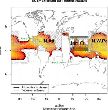
−150 −100 −50 0 50 100 150
−50
0
50
NCEP extended SST reconstruction
September/February 2005 sst$lon
sst$lat
Tropic of Cancer
Tropic of Capricorn
N.Atl. N.W.Pac
Ind.O..
September isotherms February isoterms
Fig. 1.Map showing the regions (here shown as hatched rectangles)
in whichAwas estimated together with the 26.0◦C and 26.5◦C
isotherms for February 2005 (grey) and September 2005 (black). The coloured region highlights the areal extent associated with the
September 26.0◦C isotherm, and the green dashed lines mark the
Tropics of Cancer and Capricorn.
the region 80◦W–10◦E/0◦N–40◦N (the North Atlantic) plus 100◦W–80◦W/15◦N–30◦N (Caribbean), the North-West PacificAPacover 110◦E–150◦W/0◦N–40◦N, and the Indian OceanAInd over 40◦E–110◦E/0◦N–30◦N. Figure 1 shows the isotherms for both September (largest extent in the North Atlantic) and February (smallest extent) as well as the regions in whichAwas computed (hatched regions).
The exercises were repeated with the critical threshold Tcrit set to 26.0◦C in order to examine the sensitivity to this
choice. The value ofAis insensitive to the choice of region, as long as the isotherm definingAdoes not cross the region’s boundaries.
The eastern and western border of the North-Western Pa-cific and the western border of the North Indian Ocean are nevertheless regions where the isotherms do extend beyond the selected regions, and the subjective choice of where to set these was guided by the local geography and the local character of the isotherm variability in order to minimise the sensitivity with respect toA.
−150 −100 −50 0 50 100 150
−40
−20
0
20
40
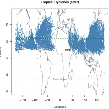
Tropical Cyclones (after)
http://www.solar.ifa.hawaii.edu/Tropical/Data/tropical Longitude
Latitude
Tropic of Cancer
Tropic of Capricorn
10N
Fig. 2. Map showing the geographical distribution of the North-ern Hemisphere tropical cyclones (cyclones in the SouthNorth-ern Hemi-sphere were not included in the data set and are hence not shown).
The black dashed line marks the 10◦N latitude and the green dashed
lines mark the Tropics of Cancer and Capricorn.
This analysis only involves TCs in the Northern Hemi-sphere. The data on North Atlantic/Caribbean (henceforth referred to as “Atlantic”) TCs (1851–2004) was taken from the National Hurricane Center6, but the TC data for the North-West Pacific (1950–2003) and the North Indian Ocean (1971–2002) were taken from US Navy best-tracks7 (Chu et al., 2002). Figure 2 also shows TC data from Hawaii8. Most of the Northern Hemisphere TCs are seen north of 10◦N, due to the fact that Coriolis force diminished towards the equator.
The sorting of TCs into the categories “N.W. Pacific” and “Indian Ocean”9 involve some uncertainties regarding storms near the 110◦E longitude (Figure 2).
2.2 Methods
The objective of this analysis was to test the hypothesis whether there is a systematic relationship between the num-ber of TCs and the warmareaof the region, where SST is greater thanTcrit=26.5◦C (here represented by the symbolA
and henceforth referred to as “the warm area”).
6http://www.aoml.noaa.gov/hrd/hurdat/hurdatTAB.txt
7http://metocph.nmci.navy.mil/jtwc/best tracks/
8http://www.solar.ifa.hawaii.edu/Tropical/Data/
9This sorting had been done at the data centre.
If it can be assumed that (i) there is no systematic change in the atmospheric conditions, (ii) that the TCs are indepen-dent of each other, and (iii) TC-formation can be represented by a stochastic process dependent on favourable SST (i.e. Bayesian type statistics), then the probability of observing a TC can be expected to be proportional toA, and the proba-bility of a TC occurrence can be expressed as:
Pr(TC|A)∝A. (3)
The expected number of TCs at any time,µ=E(N ), is then proportional to the probability, and hence the areaA. In this case, Eq. (3) represents the hypothesis which is tested here.
Since the TCs may disturb their own environment and in-fluence the large-scale setting, they are strictly not indepen-dent. It is possible that they are clustered in time as a result of weak interactions or non-linear behaviour. For instance, the convection associated with TCs may act to maintain low vertical wind shear by equalising upper and lower level hori-zontal momentum, but TCs also remove heat from the ocean surface through their action of vertical redistribution of heat. One may nevertheless expect an approximate number of TCs to be proportional toAif the probability of an event is low. The low seasonal number of cyclones and the fact that few TCs coincide in time and space are both consistent with a low probability of occurrence.
In order to reduce the influence of other factors affecting the signal-to-noise ratio, the mean seasonal cycle, rather than the individual years, was used for developing a statistical model for the relationship between the number of TCs and the warm area. If the effect from other influences (e.g. the noise) follows a Gaussian distribution, it will tend to cancel when taking the average over a long interval, as long as these are unrelated to the seasonal cycle or the SST itself. This strategy is inspired by similar approaches used in instrumen-tation, where phase-locking and “choppers” with predefined frequencies improve the signal-to-noise ratios (e.g. in optics). Furthermore, the low number of TC-events for each month or season, which in reality reflects a low probability Pr(TC|A), hampers any attribution analysis. An average over longer interval improves the statistical power, but the ques-tion has to be addressed concerning whether the calibraques-tion is biased by other factors also exhibiting an annual cycle not related to SST.
3 Results
It is possible that both respond to the seasonal variation in the angle of solar inclination, however, this would suggest that the response would peak in June for latitudes greater than the Tropic of Cancer10 in the Northern Hemisphere, unless there is a similar lag in the SST and TC response.
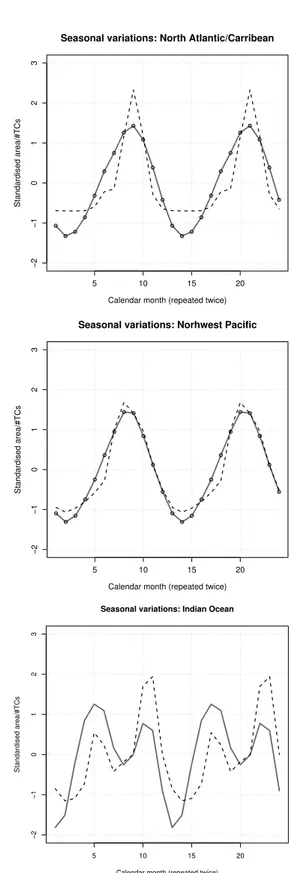
Due to high heat capacity, the oceans are expected to react more slowly, but the atmosphere tends to respond almost in-stantaneously. Hence, the same phase lag in the two curves may suggest that the variation in the number of TCs may be influenced by the oceanic state, and only indirectly by the seasonal variation in the solar angle of inclination. In the North Atlantic, the peak inNAtlandAAtlis seen in Septem-ber when the annual variation in the oceanic heat content is at maximum (the same month in the year as the sea-ice extent in the Arctic is at minimum), while in the North-West Pa-cific (Fig. 3b),APacandNPacpeak in August (APacis slightly greater in August than in September).
An interesting observation is that there is not a one-to-one ratio betweenN andA. For the Atlantic region, there is a disproportionally high numberN for the month with great-est areaA. Thus, the hypothesis (Eq. 3) that the number of TCs is proportional to the warm area therefore appears to be inconsistent with these results.
For the North-West Pacific, on the other hand, the annual cycle ofNPacandAPacexhibits more of a linear relationship, however, the peak in TC number is still narrower than that of the warm area.
Over the North Indian Ocean, the seasonal cycle is charac-terised by a double peak in both temperature-weightedAInd andNInd(Fig. 3c), however, the second peak inNIndis more pronounced than the first, whereas the first peak forAIndis more prominent than the second. Furthermore, the second annualN peak in the Indian Ocean lagsAby one month.
The relationship between the warm surface area and the number of cyclones can be explored further through slightly more sophisticated statistical analysis. The loga-rithm of the seasonal variation in warm Atlantic surface area (x=log(A)) is compared with the logarithm of the sea-sonal cycle in monthly mean number of Atlantic TCs,NAtl (y=log(N )), and a regression was carried out based on the modelyˆm=αxm+β, wheremrepresents the different months
in the TC season.
Here a linear relationship was derived between the mean seasonal cycle ofxandytaken over the interval 1944–2004. Only the months withy=ln(N )>−3 (May–December) were used to calibrate the model. The relationship betweenx and y has a predominately linear character (Fig. 4) that implies the expression:
NAtl∝A5Atl.06±0.25. (4) The linear least-squares regression analysis returned a p-value for this relationship of the order 10−6, adjusted
10Located at 23.5◦north of the equator.
5 10 15 20
−2
−1
0
1
2
3
Seasonal variations: North Atlantic/Carribean
Calendar month (repeated twice)
Standardised area/#TCs
5 10 15 20
−2
−1
0
1
2
3
Seasonal variations: Norhwest Pacific
Calendar month (repeated twice)
Standardised area/#TCs
5 10 15 20
−2
−1
0
1
2
3
Seasonal variations: Indian Ocean
Calendar month (repeated twice)
Standardised area/#TCs
Fig. 3. The annual variation in surface area of SST >26.5◦C
(A; grey) and the number of TCs (N; dashed) for the (a)
At-lantic/Caribbean basin,(b)the North-West Pacific, and(c)the
In-dian Ocean, but for a temperature-weighted area (AT). All the
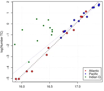
16.0 16.2 16.4 16.6 16.8
−4
−3
−2
−1
0
1
The Atlantic basin
Years calibr. 1944 − 2004 , years eval. before 1944log(Area)
log(Number TC)
y < −3 Calibr. train Independent
Fig. 4. Scatter-plot of seasonal values x=log(A) andy=log(N)
for the Atlantic basin. HereAis in units of km2 andN in
num-ber/month. Both calibration (dependent) and independent data are
shown. Only the months with ln(N )>−3 were used to estimate the
best-fit, but these months are also shown as open symbols (indepen-dent validation data).
R2=0.98, andF-statistic of 398 on 1 and 6 degrees of free-dom (DF). The same tendency was seen in the independent data over the 1851–1943 period (red symbols in Fig. 4) and the months with very few TCs (open symbols).
The figure shows less than 12 data points for each ocean basin, but each value is a mean estimate of many measure-ments. The fact that the older independent data shows the same statistical pattern as the calibration data suggests that a deterioration in the data quality, if present, does not have a strong effect on this analysis.
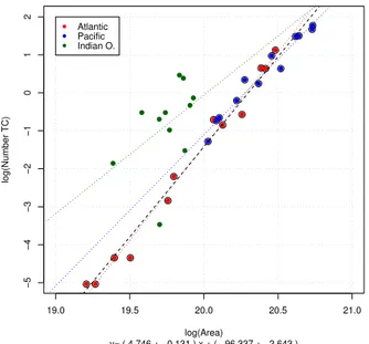
Figures 5–7 show a combined log-log scatter plot for the three ocean basins, and the relationships revealed in this plot point to some intriguing features. The data representing the North-West Pacific indicates similar linear relationship be-tween the x andy as in the North Atlantic/Caribbean, but the slope is slightly weaker:NPac∝A4Pac.44±0.37(Adjusted R-squared=0.93,F-statistic=146 on 1 and 10 degrees of free-dom, andp-value=2.7×10⁻⁷).
The relationship over the North Indian Ocean is poor although the best-fit suggested NInd ∝ A3Ind.46±1.50 (Ad-justedR-squared=0.35,F-statistic=5 on 1 and 7 DF, and p-value=0.05). The double peaks in bothAInd andNInd are somewhat consistent with a close association, but the phase match is not perfect as the secondNIndpeaks one month later than correspondingAT (Fig. 3c), and the magnitudes of the
peaks are not consistent. Furthermore, the log-log points in Fig. 4 fall outside the linear fit.
16.0 16.5 17.0
−5
−4
−3
−2
−1
0
1
2
y= ( 4.876 +− 0.131 ) x + ( −82.719 +− 2.196 )log(Area)
log(Number TC)
Atlantic Pacific Indian O.
Fig. 5. Scatter-plot of seasonal valuesx=log(A) andy=log(N) for
the Atlantic, North-West Pacific and Indian ocean basins. HereAis
in units of km2andNin number/month and the calibration of the
fits and the data presented involve all available data. The dashed lines show the best linear-log fits, where the black line represents the combined fit for the Atlatnic and the North-West Pacific.
So far, the possibility that other factors important for TCs also exhibiting an annual cycle cannot not be ruled out, de-spite the similar phase lag forNAtlandAAtlwith respect to solar inclination angle.
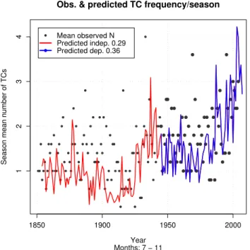
One way to isolate and assess the importance of the warm sea area with respect toN is then to use the statistical rela-tions derived above to predict year-to-year variarela-tions in the seasonal mean number of TCs over an interval represent-ing independent data, and subsequently evaluate against the observations (Fig. 8). This kind of approach was used by Michaels et al. (2006) to assess the association between SST and the total number of annual TCs, however, here the SSTs (in their analysis averaged over 10◦N–25◦N and 15◦W– 80◦W) were substituted with the predicted values using ex-pression 4 (note, the conclusions drawn here contrast with those made by Michaels et al., 2006). One limitation is that Eq. (4) only gives an approximate value, as the relationship is non-linear, and the seasonal mean value may not capture high values associated with highAin individual months.
When the simple model (Eq. 4) was applied to the hurricane-season meanAAtl(June–November) of each year over the 1944–2004 interval (blue curve), a correlation of 0.35 was achieved (p-value=0.005, assuming independent and identically distributed data). The results were not sensitive to the particular choice for critical threshold, as when Tcrit=26.0◦C was used, the correlation was 0.37
19.0 19.5 20.0 20.5 21.0
−5
−4
−3
−2
−1
0
1
2
y= ( 4.746 +− 0.131 ) x + ( −96.337 +− 2.643 ) log(Area)
log(Number TC)
Atlantic Pacific Indian O.
Fig. 6.Scatter-plot of seasonal valuesx=log(AT) andy=log(N) for the Atlantic, North-West Pacific and Indian ocean basins. Here the
temperature-weightedAT is in units of◦C×km2andN in
num-ber/month and the calibration of the fits and the data presented in-volve all available data. The dashed lines show the best linear-log fits, where the black line represents the combined fit for the Atlatnic and the North-West Pacific.
For the older data (representing 1851–1943; red curve) with presumed lower quality, the analysis withTcrit=26.5◦C
gave a weaker correlation (r=0.28), but it was still statisti-cally significant at the 1% level (p-value=0.008;Tcrit=26.0◦C
gaver=0.29 withp-value=0.006).
In other words, the empirical expression captures some of the year-to-year variations in the TC numbers over the inde-pendent evaluation period. The area of high SST do by no means explain most of the year-to-year variability, and the large differences between the predictions and observations also suggest that other factors are important in determining N.
A similar correlation analysis for the North-West Pa-cific over the independent years 1950–1987 yielded a weak correlation (r=0.23) with a p-value of 0.17 (Tcrit=26.0◦C:
r=0.11 with a p-value=0.53), and a negative correlation (r=−0.29) for the Indian Ocean over the interval 1971–1992 (p-values=0.18)11. These results are similar to the correla-tions between regional mean SSTs and the ACE found by Klotzbach (2006), with positive correlations in the North At-lantic and North-West Pacific and negative over other ocean basins.
An assessment of the number of TCs estimated according to Eq. (4), based on the trend inAAtl, also appears to provide a rough description of the long-term trend: When taking a polynomial trend (Benestad, 2003) inA(Fig. 9, left panel)
11ForT
crit=26.0◦C the same correlation for the Indian Ocean gave
−0.27 (p-values=0.20)
16.0 16.2 16.4 16.6 16.8 17.0
−5
−4
−3
−2
−1
0
1
2
y= ( 4.758 +− 0.784 ) x + ( −79.244 +− 12.942 )log(Area)
log(Number TC)
Atlantic Pacific Indian O.
Fig. 7. Scatter-plot of seasonal values x=log(Aτ) andy=log(N) for the Atlantic, North-West Pacific and Indian ocean basins. Here
the peak-over-thresholdAτ is in units of◦C×km2andNin
num-ber/month and the calibration of the fits and the data presented in-volve all available data. The dashed lines show the best linear-log fits, where the black line represents the combined fit for the Atlatnic and the North-West Pacific.
as input for Eq. (4), the predictions provide a reasonable de-scription of the long-term evolution in the number of TCs (right panel), with the exception before 1900. The simple statistical model based on this expression (Eq. 4) captures the rapid increase in the number of TCs for the 2005 season, as well as weak trends in the past.
A similar analysis with temperature-weighted area (AT(t )=Pijwjγij(t )×H(Tij(t )−Tcrit)), where each
grid-box was scaled by Tij(t ) (in ◦C) gave similar results,
al-though improved correlations for the North-West Pacific (for Tcrit=26.0◦C r=0.29 with a p-value=0.07 over the
in-dependent years 1950–1987). Since the temperature in the grid-box where Tij(t )≥Tcrit are of similar magnitude
(26◦C<γij(t )=Tij(t )<35◦C), the effect of the scaling only
modifies the area-based analysis. When the peak over thresh-old (γij(t )=Tij(t )−Tcrit) were used as scaling, however, then
the results suggested a weak relationship.
4 Discussion
1850 1900 1950 2000
1234
Obs. & predicted TC frequency/season
Months: 7 − 11 Year
Season mean number of TCs
Mean observed N Predicted indep. 0.29 Predicted dep. 0.36
Fig. 8.Observed and predictedNfor the Atlantic, based on Eq. (4).
Correlation coefficients are provided in the legend (Tcrit=26.5◦C).
It is possible that the relationship found here may be more complicated than it first appears, as other conditions also undergoing similar annual cycles may introduce misleading biases in the end results. On the other hand, factors other than SST that may affect TCs are most likely not indepen-dent of the SSTs (shear, humidity, CAPE, El Ni˜no, etc.), so that the area of the warm sea may also be regarded as proxy for all these aspects (Chauvin et al., 2006). Klotzbach and Gray (2008) argued, however, that the statistical description is improved by combining sea-level pressure with SST in the statistical analysis of TCs.
One interesting aspect is the tendency of similar linear log-log relationship betweenN andAin the Pacific Ocean and the Atlantic, but a different character in the Indian Ocean basin. Holland (1997) suggested that different mechanisms may be operating in different ocean basins, and Yoshimura et al. (2006) found from model studies that there may be dif-ferent response in the TC statistics to a global warming. For instance, the El Ni˜no Southern Oscillation (ENSO) has dif-ferent effects on tropical cyclones in the North-West Pacific and the North Atlantic.
The different oceans are characterised with different dy-namics (ocean currents), geometry, and overlying atmo-spheric circulation (e.g. monsoon systems, easterly waves), all of which may play a role in terms of cyclogenesis. Fur-ther work is required to discriminate the role of atmospheric processes from the effect ofA. So far, only similar phase lag in the annual cycle and independent year-to-year correlation analysis suggest a connection.
The statistical models trained on seasonally varying values (Eq. 4) did not yield skillful predictions for year-to-year vari-ations inN over the North Indian Ocean. The reason for the negative correlation between predicted and observed year-to-year variations inNIndmay be associated with the different magnitudes in the double-peak structure, weak statistical re-lation, and the large scatter in seen in Fig. 5. Furthermore, the phase match between N andAwas not perfect for the Indian Ocean.
The physical explanation for this may be the small an-nual variations in A, constraints imposed by the northern boundary, or that the variations in SST above the threshold value mainly take place southward of the Tropic of Can-cer. The northern boundary of the Indian Ocean is close to the Tropic of Cancer (Fig. 1), and southward of this lat-itude the solar inclination angle reaches a maximum twice a year. Hence much of the variation in the North Indian Ocean warm sea region may take place southward of 23.5◦N, where the solar inclination is expected to exhibit a double peak. Furthermore, the southwest Asian Monsoon has a sim-ilar twice-a-year wind reversal over the Indian Ocean, and the Indian Ocean winds influence the seasonal evolution of surface fluxes, convection, and ultimately affect the SSTs. There is a close coupling between the tropical ocean and the atmosphere.
The value for N over the Indian Ocean was in general above the predictions onAin Fig. 5, which is also consis-tent with the explanation that some TCs may originate in the Pacific basin but end up in the Indian Ocean.
It is also possible that the low year-to-year correlation and low statistical significance for the Indian Ocean and the North-West Pacific may be a result of lower data qual-ity in these basins (Landsea et al., 2006), shorter series, or due to stronger influence from other factors such as atmo-spheric conditions not directly related to the warm pool area (Chan, 2006; Klotzbach, 2006). Both the Indian Ocean and North-West Pacific records are short compared to the At-lantic record, and the annual cycles are hence more strongly affected by noise.
There are further limitations to the data on which this anal-ysis rests, as the TC series should not be considered ho-mogeneous. The Atlantic TC data after 1944 is thought to have higher quality than the earlier observations (Goldenberg et al., 2001), however, the hurricane record is most reliable after 1970 (Trenberth et al., 2007).
The ability to detect TCs in the open Atlantic has increased substantially over time as aircraft reconnaisance and (in the 1970s) satellite monitoring have become available. These improvements in detection tools may have led to enhanced probability of detection of weak and remote TCs over time, although estimated maximum potential intensities of tropical cyclones appear to show some agreement with the observa-tions (Henderson-Sellers et al., 1998).
1850 1900 1950 2000
1.8e+07
2.0e+07
2.2e+07
2.4e+07
Area of Atlantic warm region
Months: 7 − 11Time
Area (km^3)
1850 1900 1950 2000
1234
TC frequency
Months: 7 − 11Year
Season mean number of TCs (#/month)
Mean observed N Predicted trend
Fig. 9. (a)The area of the Atlantic warm regionAand(b)a reconstruction of the trend inN for historic Atlantic TCs based on trend in
NAtl∝A6Atl.64. Here a polynomial trend model was used because of the non-linear relationship betweenAAtlandNAtl. HereAis in units of
km2andNin number/month (Tcrit=26.5◦C).
that an improved Dvorak technique due to the introduc-tion of IR measurements has enhanced the quality of the maximum wind estimates since 1984. Thus, there may be inhomogeneities introduced by problems in measuring and estimating the hurricane intensities due to satellite improve-ments (Landsea et al., 2006), but a comparison with older in-dependent data (Fig. 4) suggests that analysis presented here is not sensitive to such inhomogeneities.
Using the seasonal variations inAandNdefined over the 1944–2004 interval will to some extent also alleviate prob-lems associated with inhomogeneities in the TC record. The fact that the correlation analysis between predictions based on Eq. 4 and actual observations yielded results significant at the 1%-level forindependent(older) data, provides strong support for the statistical model established here for the At-lantic/Carribean basin. Evaluation against independent data by dividing the data in to two periods, is a more stringent test than simply using cross-validation (Wilks, 1995). Further-more, months with lowN (y<−3) were excluded from the model training, but also these are approximately in line with the model predictions.
The warm area cannot account for all the variability and other factors, such as atmospheric conditions, also affect the number of TCs. An intriguing question is whether the annual variation of such factors are independent or affected by the warm area. Chauvin et al. (2006) found that the SSTs had a significant effect on the TC statistics, but was not the only factor. Their results suggested that the spatial SST structure was important as well as the magnitude.
Increases in the convective available potential energy (CAPE) are associated with increased near-surface temper-ature (Gettelman et al., 2002), suggesting that an increased warm area may enhance convection over a greater region and hence cause a more widespread vertical equalisation of hor-izontal momentum, and thus act to reduce the vertical shear. Hence, the role TCs play in the vertical redistribution of mo-mentum and their effect on the ambient atmosphere may en-hance the conditions of TC formation and growth. It is there-fore plausible that the TCs are organised in time clusters, where the presence of one TC creates conditions that may favour the genesis of subsequent TCs, given sufficiently large area over which they can form. It is also plausible that a ver-tical re-distribution of heat and moisture, as a result of TC activity may, on the other hand, inhibit further TCs, if TCs equalise the vertical distribution of heat through some kind of “discharge mechanism”.
Another speculation is whether time clustering of TCs may be associated with a modulation of TC occurrence by the Madden-Julian Oscillation (MJO), or conversely that the MJO is affected by the TCs.
convection starts to achieve a certain circular structure may spawn cyclones. Furthermore, the geography will provide an upper bound for the TC numbers (especially for the Northern Indian Ocean).
For a stochastic and static process, the number of events (k) is expected to be distributed according to the Poisson dis-tribution: Pr(X=k|A)=µkke!−µ. The question of how to regard µin the case of TCs, as an average over timeµ=µor a vari-ableµ=µ(t ) conditioned by changing external conditions, has a bearing on howN should be modelled statistically. If µvaries withA, e.g. from season to season, one cannot ex-pect the distribution for all historical TCs to follow a Poisson distribution if all events are put into one single batch.
Finally, a non-linear relationship betweenAandN may explain why linear trends in the TC frequency has not been detected in the past: There is a substantial response inNonly whenAreaches a certain size.
The non-linear relationship implies one caveat: taking the mean A over a season will not provide an exact esti-mate ofN over the same season for a non-linear relationship (N (t )=cRtAx(t )dt6=cAxt), especially for high values ofA. Thus, these results should only be regarded as approximate.
These results may seem to disagree with most GCM-based studies (Meehls et al., 2007; Chauvin et al., 2006; Yoshimura et al., 2006), but this analysis only took into account varia-tions in the warm area, and changes in the atmospheric en-vironments do also play a role. Competing effects, such as greater hydrostatic stability, and wind shear may counter-act the effect of higher SSTs. However, these findings seem to be in line with Lau et al. (2008).
High-resolution model studies also indicate reduction in the global number of TC, but the models must demonstrate that they reproduce both the past trends in the TC statistics as well as the seasonal relationships presented here, in order to prove that they give a representative picture of TCs. At the present, the GCMs do not reproduce the observed SST-wind relationships (Yoshimura et al., 2006), and may be too sensitive to the cloud parameterisation schemes.
Vecchi et al. (2008) argue that the effect of a global warm-ing – both for the past and in the future – on the tropical Pacific is highly uncertain, as some studies suggest a shift to-wards a state more like La Ni˜na (mainly oceanic processes) while others (atmospheric processes) point to a more El Ni˜no like state. Furthermore, depending on whether one looks at the HadISST or the NOAA extended reconstruction of SST, one finds that the shift in the past has been towards a more La Ni˜na or El Ni˜no like state, respectively. Thus, the uncer-tainty in the long-term changes will likely have consequences for the evolution in ENSO, and hence the TC statistics in some ocean basins. It is at present not possible to resolve the issues regarding the homogeneity in either the TC or SST record. Nevertheless, the statistical patterns identified in this analysis are interesting.
This study involved no physical basis as such, as it merely presented empirical data in a new fashion to outline some intriguing features. The results derived here falsify two hy-potheses: (i) that TCs are random and (ii) thatN is insensi-tive toAas claimed by Henderson-Sellers et al. (1998).
5 Conclusions
Here empirical data has been organised and presented in a new fashion. The correlation analyses between predictions and year-to-year variations in the seasonal mean TC-number suggest that a simple statistical model, based on the warm sea area, captures a part of the variations over the North Atlantic and Caribbean basins, to a lesser degree over the North-West Pacific, but not over the North Indian Ocean. For the At-lantic basin, these results are inconsistent with TCs being purely stochastic processes taking place over warm ocean regions, and provide strong evidence for a real connection betweenN andA. Thus, these conclusions are inconsistent with the claim that the region of cyclogenesis will not expand with the 26.5◦C isotherm. These results furthermore suggest that there may be a non-linear relationship between the area of high SST and the number of TCs in some ocean basins, which can explain why there in the past has not yet been a clear linear upward trend in the number of TCs associated with the general warming. It also explains the recent upturn in the number of TCs. One important caveat of this study is that it is based purely on a limited selection of empirical data.
Acknowledgements. The work has been supported by “Norsk Meteorolog Forening” and to some extent by the Norwegian Mete-orological Institute, as much of this work was done during travels to Utrech (EMS), Berlin, and Helsinki. Inputs from E. A. Smith, NASA/GSFC and A. V. Mehta through the review process and Ø. Nordli have been valuable.
Edited by: A. Mugnai Reviewed by: E. A. Smith
References
Benestad, R. E.: What can present climate models tell us about climate change? Climatic Change, 59, 311–332, 2003.
Benestad, R. E., 2006: An explanation for the lack of trend in the hurricane frequency, arXiv: physics/0603195., http://arxiv.org/ abs/physics/0603195, March 2006.
Bengtsson, L., Hodges, K. I., and Roeckner, E., Storm Tracks and Climate Change, J. Climate, 19, 3518–3542, 2006.
Chan, J.: Comments on “Changes in Tropical Cyclone Number, Duration, and Intensity in a Warming Environment”, Science, 311, 1713b, doi:10.1126/science.1121522, 2006.
Chronis, T., Williams, E., Anagnostou, E., and Petersen, W.: African Lightning: Indicator of Tropical Atlantic Cyclone for-mation, Eos, 88, 397–398, doi:10.1029/2007EO400001, 2007. Chu, J.-H., Sampson, C. R., Levin, A. S., and Fukada, E.: The
Joint Typhoon Warning Center tropical cyclone best tracks 1945– 2000 report, Joint Typhoon Warning Cent., Pearl Harbor, Hawaii, 2002.
Emanuel, K.: Increasing destructiveness of tropical cyclones over the past 30 years, Nature, 436, 686–688, 2005.
Gettelman, A., Seidel, D. J., Wheeler, M. C., and Ross, R. J.: Mul-tidecadal trends in tropical convective available potential energy, J. Geophys. Res., 107(D21), 4606, doi:10.1029/2001JD001082, 2002.
Goldenberg, S. B., Landsea, C. W., Mestas-Nunez, A. M., and Gray, W. M.: The recent Increase in Atlantic Hurricane Activ-ity: Causes and Implications, Science, 293, 474–479, 2001. Gray, W. M.: A global view of the origin of tropical disturbances
and storms, Mon. Weather Rev., 96, 669–700, 1968.
Henderson-Sellers, A., Zhang, H., Berz, G., Emanuel, K., Gray, W., Landsea, C., Holland, G., Lighthill, J., Shieh, S.-L., Web-ster, P., and McGuffie, K.: Tropical Cyclones and Global Climate Change: A Post-IPCC Assessment, B. Am. Meteorol. Soc., 79, 20–38, 1998.
Holland, G. J.: The maximum potential intensity of tropical cy-clones, J. Atmos. Sci., 54, 2519–2541, 1997.
Holland, G. J.: Misuse of Landfall as a Proxy for Atlantic Tropical Cyclone Activity, Eos, 88, 349–356, 2007.
Hoyos, C. D., Agudelo, P. A., Webster, P. J., and Curry, J. A.: De-convolution of the Factors Contributing to the Increase in Global Hurricane Intensity, Science, 312, 94–97, 2006.
Jung, T., Gulev, S. K., Rudeva, I., and Soloviov, V.: Sensitivity of extratropical cyclone characteristics to horizontal resolution in the ECMWF model, Research Dept., Technical Memorandum 485, ECMWF, 2006.
Klotzbach, P. J.: Trends in global tropical cyclone activity over the past twenty years (1986–2005), Geophys. Res. Lett., 33, L10805, doi:10.1029/2006GL025881, 2006.
Klotzbach, P. J. and Gray, W. M.: Multidecadal Variability in North Atlantic Tropical Cyclone Activity, J. Climate, 21, 3929–3935, doi:10.1175/2008JCLI2162.1, 2008.
Knutson, T. R. and Tuleya, R. E.: Impact of CO2-Induced Warming
on Simulated Hurricane Intensity and Precipitation: Sensitivity to the Choice of Climate Model and Convective Parameteriza-tion, J. Climate, 17, 3477–3495, 2004.
Knutson, T. R. and Tuleya, R. E.: Reply, J. Climate, 18, 5183–5187, 2005.
Landsea, C. W., Harper, B. A., Hoarau, K., and Knaff, J. A.: Can we detect trends in extreme tropical cyclones?, Science, 313, 452– 454, 2006.
Landsea, C. W.: Counting Atlantic Tropical Cyclones Back to 1900, Eos, 88, 197–202, 2007.
Lau, K. M., Zhou, Y. P., and Wu, H. T.: Have tropical cyclones been feeding more extreme rainfall?, J. Geophys. Res., 113, D23113, doi:10.1029/2008JD009963, 2008.
Lau, W. K. M. and Kim, K.-M.: How Nature Foiled the 2006 Hur-ricane Forecasts, Eos, 88(9), 105–107, 2007.
Mann, M. E., Emanuel, K. A., Holland, G. J., and Webster, P. J.: Atlantic Tropical Cyclones Revisited, Eos, 88(36), 49 pp., 2007. Meehls, G. A., Stocker, T. F., Idlingstein, W. D., Gaye, A. T., Gre-gory, J. M., Kitoh, A., Knutti, R., Murphy, J. M., Noda, A., Raper, S. C. B., Watterson, I. G., Weaver, A. J., and Zhao, Z.-C.: Climate Change: The Physical Science Basis, United Kingdom and New York, NY, USA, Cambridge University Press, Chap. Global Climate Projections, 2007.
Michaels, P. J., Knappenberger, P. C., and Davis, R. E.: Sea-surface temperatures and tropical cyclones in the Atlantic basin, Geo-phys. Res. Lett., 33, L09708, doi:10.1029/2006GL025757, 2006. Pearce, R.: Comments on “Why must hurricanes have eyes?” –
revisited, Weather, 60(11), 329–330, 2005a.
Pearce, R.: Why must hurricanes have eyes? Weather, 60(1), 19–24, 2005b.
Randall, D. A., Wood, R. A., Bony, S., Colman, R., Fichefet, T., Fyfe, J., Kattsov, V., Pitman, A., Shukla, J., Srinivasan, J., Stouf-fer, R. J., Sumi, A., and Taylor, K. E.: Climate Change: The Physical Science Basis, Cambridge, UK: Cambridge University Press, Chap. Climate Models and Their Evaluation, 2007. Scharroo, R., Smith, W. H., and Lillibridge, J. L.: Satellite
Altime-try and the Intensification of Hurricane Katrina, Eos, 366 pp., 2005.
Scharroo, R., Smith, W. H. F., and Lillibridge, J. L.: Reply to Com-ment on “Satellite Altimetry and the Intensification of Hurricane Katrina”, Eos, 87(8), 89 pp., 2006.
Smith, R. K.: “Why must hurricanes have eyes?” – revisited, Weather, 60(11), 326–328, 2005.
Sun, D., Gautam, R., Cervone, G., Boybeyi, Z., and Kafatos, M.: Comment on “Satellite Altimetry and the Intensification of Hur-ricane Katrina”, Eos, 87(8), 89 pp., 2006.
Trenberth, K.: Uncertainty in Hurricanes and Global Warming, Sci-ence, 308, 1753–1754, 2005.
Trenberth, K. E., Jones, P. D., Ambenje, P., Bojariu, R., Easterling, D., Klein Tank, A., Parker, D., Rahimzadeh, F., Renwick, J. A., Rusticucci, M., Soden, B., and Zhai, P.: Climate Change: The Physical Science Basis, Cambridge, UK, Cambridge University Press, Chap. Observations: Surface and Atmospheric Climate Change, 2007.
Vecchi, G. A., Clement, A., and Soden, B.: Examining the Tropical Pacific’s Response to Global Warming, Eos, 89(9), 81 pp., 2008. Vitard, F., Stockdale, T., and Ferranti, L.: Seasonal forecasting of
tropical storm frequency, ECMWF Newsletter, 16–22, 2007. Webster, P. J., Holland, G. J., Curry, J. A., and Chang, H.-R.:
Changes in Tropical Cyclone Number, Duration, and Intensity in a Warming Environment, Science, 309, 1844–1846, 2005. Wilks, D. S.: Statistical Methods in the Atmospheric Sciences,
Or-lando, Florida, USA, Academic Press, 1995.
Wu, M-.C., Yeung, H., and Chang, W-.L.: Trends in Western North Pacific Tropical Cyclone Intensity, Eos, 87(48), 537 pp., 2006. Yoshimura, J., Masato, S., and Noda, A.: Influence of Greenhouse