Mathematical modelling to assess the carrying capacity for
multi-species culture within coastal waters
P. Duarte
a,∗, R. Meneses
a, A.J.S. Hawkins
b, M. Zhu
c, J. Fang
d, J. Grant
eaIMAR—Departamento de Ciˆencias e Engenharia do Ambiente, Universidade Nova de Lisboa, 2825-114 Monte de Caparica, Portugal bPlymouth Marine Laboratory, Prospect Place, The Hoe, Plymouth PL1 3DH, UK
cState Oceanic Administration, First Institute of Oceanography, Xianxialing Road, 266061 Qingdao, PR China dYellow Sea Fisheries Research Institute, 106 Nanjing Road, 266071 Qingdao, PR China
eDepartment of Oceanography, Dalhouise University, Halifax, NS, Canada B3H 4J1
Received 7 May 2002; received in revised form 21 March 2003; accepted 20 May 2003
Abstract
In the context of aquaculture, carrying capacity is generally understood as the standing stock of a particular species at which production is maximised without negatively affecting growth rates. The estimation of carrying capacity for aquaculture is a complex issue. That complexity stems from the many interactions between and among cultivated and non-cultivated species, as well as between those species and their physical and chemical environments. Mathematical models may help to resolve these interactions, by analysing them in a dynamic manner. Previous carrying capacity models have considered the biogeochemical processes that influence growth of cultivated species in great detail. However, physical processes tend to have been addressed very simplistically. Further, most modelling has been for monocultures, despite the increasing importance of multi-species
(=polyculture) systems.
We present here a two-dimensional coupled physical–biogeochemical model implemented for Sungo Bay, Shandong Province, People’s Republic of China. Sungo Bay is used for extensive polyculture, where bivalve shellfish and kelp are the most important cultivated species. Data collected over 13 years (1983–2000) was available for modelling. Our main objectives were to implement the model, achieving reasonable calibration and validation with independent data sets, for use in estimating the environmental carrying capacity for polyculture of scallops and oysters.
Findings indicate that the model successfully reproduces some of the main features of the simulated system. Although requiring some further work to improve predictive capability in parts, predictions clearly indicate that Sungo Bay is being exploited close to the environmental carrying capacity for suspension-feeding shellfish. Comparison of different culture scenarios also indicates that any significant increase in yield will depend largely on a more optimal spatial distribution of the different cultivated species. © 2003 Elsevier B.V. All rights reserved.
Keywords:Ecological modelling; Carrying capacity; Multi-species culture
∗Corresponding author. Present address: CEMAS—University Fernando Pessoa, Praça 9 de Abril 349, 4249-004 Porto, Portugal. Tel.:+351-22-507-1300; fax:+351-22-550-8269.
E-mail address:pduarte@ufp.pt (P. Duarte).
1. Introduction
Estuaries and semi-enclosed bays are inten-sively used for aquaculture in many countries. Suspension-feeding bivalves are among the most cultivated organisms in these ecosystems. This is a “passive” type of culture, where the animals feed
on natural suspended matter, their metabolites being dispersed by currents and waves.
The concept of environmental carrying capacity is not only important for species cultivation but also for other concerns such as water quality and tourism. With respect to bivalve culture, carrying capacity has been defined as the maximum standing stock that may be kept within a particular ecosystem to max-imise production without negatively affecting growth
rate (Carver and Mallet, 1990). Alternatively, and
more recently, carrying capacity has been described as the standing stock at which the annual production
of the marketable cohort is maximised (Bacher et al.,
1998). There are several other definitions of carrying
capacity for aquaculture in the literature. However, these are generally concerned with the culture of a single target species, despite a growing tendency in Eastern Countries for “ecological aquaculture” based on multi-species culture, where producers and consumers are grown together to facilitate nutrient recycling. Here, the objective is not only to maximise production, but also to optimise species combina-tions and distribucombina-tions in such a way as to reduce the environmental impacts of aquaculture. The growing appreciation that ecosystems have multiple functions, with a need for integrated management, means that ecologists are increasingly challenged to model the many interactions between and among species, in-cluding with their environment, on a large scale. A general definition of carrying capacity at the ecosys-tem level could be “the level to which a process or variable may be changed within a particular ecosys-tem, without driving the structure and function of the ecosystem over certain acceptable limits”. The defini-tion of “acceptable limits” is very difficult. However, once established in terms of water quality and other parameters, it should be possible to manage different ecosystem uses in a sustainable manner.
There are several examples where carrying ca-pacities for bivalve cultivation have been exceeded by non-sustainable practices. These include the bay
of Marénnes-Óleron (France), where oyster (
Cras-sostrea gigas) growth has reduced significantly with
increased stock densities over the years (Raillard and
Ménesguen, 1994). Similarly, mussel (Mytilus edulis) growth in the Oosterschelde estuary (The Nether-lands) has been compromised by increased standing
stocks (Smaal et al., 2001).
Carrying capacities for the culture of suspension-feeding bivalves are primarily limited by rates with which available food is renewed, which is a function of phytoplankton production and water residence time (Dame and Prins, 1998). It is also important to con-sider the impact of bivalve cultivation itself on water quality, sediment composition and ecosystem func-tioning. By recycling nitrogen, bivalves may stimulate
primary productivity (Smaal et al., 2001). For the
same reasons, in line with the concept of ecological aquaculture, bivalves may be successfully cultured alongside kelp, when nutrients excreted and egested by the bivalves may be absorbed by macroalgae and
recycled into valuable biomass (Fang et al., 1996).
The dynamics of multi-species culture is complex, with many potential positive and negative feedbacks between the cultivated and the non-cultivated species. These feedbacks must be considered when the goal is to optimise production and minimise ecological impacts. For example, macroalgae may compete with phytoplankton for nutrients, and any reduction in phytoplankton biomass may have a negative impact on bivalve growth. In addition, aquaculture structures like rafts and ropes impose drag, thereby reducing current flow and the renewal both of suspended
parti-cles for bivalves and of nutrients for kelp (Grant and
Bacher, 2001).
To manage such a complex system, these interrela-tions must all be taken into account. Further, the only way to integrate these interactions is by means of mathematical modelling. Given that different species are distributed in different areas according to their en-vironmental requirements or other criteria, it is impor-tant that the models are spatially resolved. Typically, spatially resolved ecological models simulate hydro-dynamic transport in a very simple way, considering residual flows and tidally averaged situations. These
are known as box models (e.g.Bacher, 1989; Raillard
and Ménesguen, 1994; Ferreira et al., 1998). For a de-scription of the general structure of an ecosystem box
model with bivalve suspension feeders see Herman
(1993)andDowd (1997). The upscaling of physical transport from hydrodynamic models of high spatial and temporal resolution to biogeochemical models
of coarser resolution, as described inJørgensen and
Bendoricchio (2001), has been used by several au-thors for bivalve carrying capacity modelling (e.g.
Until recently, relatively little modelling work has been done on the interface between hydrodynamics and biogeochemistry using fully coupled models in
marine ecosystems (Dike, 2001). Perhaps one of the
most complex ecological models so far developed for a coastal ecosystem was that of the Ems estuary (Baretta and Ruardij, 1988). In spite of the degree of biogeochemical detail present in this model, the phys-ical environment is described in a relatively simple way, using residual flows and diffusion coefficients to parameterise transport.
Although useful in many different ways, box models generally fail to reproduce some important dynamic processes that may affect ecosystem func-tioning. Among others, these include tidal height vari-ability and its influence on underwater light intensity, as well as current speed dynamics and its influence on sediment resuspension processes, on water turbid-ity and on water renewal at small spatial scales. The solution to these problems is to have fully coupled
Fig. 1. The location of Sungo Bay, including model domain and bathymetry (m). Also shown, is a part of the model grid (upper left corner), with spatial resolution of 500 m.
physical–biogeochemical models that simulate hydro-dynamic transport phenomena including chemical and biological processes within a common framework.
From a practical standpoint, it is very difficult if at all possible to optimise multi-species cul-ture through trial and error. Instead, fully coupled physical–biogeochemical models will enable the comparative assessment of different aquaculture sce-narios. Model outputs may then be used to design field trials that may in turn feedback to the models. Iterative application of modelling, field trials and ex-periments will help to develop understanding of the studied ecosystems, facilitating a more sustainable culture practice.
Main objectives of the work described here were to:
(1) develop a two-dimensional coupled physical– biogeochemical mathematical model for Sungo Bay, Shandong Province, People’s Republic of
suspension-feeding bivalves and kelps, including their interactions with the ecosystem;
(2) calibrate and validate the model with separate data sets;
(3) use the model to assess how current culture prac-tice compares with environmental carrying capac-ity of the bay;
(4) use the model to analyse the consequences of sev-eral possible culture practices for bivalve produc-tion in Sungo Bay; and
(5) assess whether our estimates of carrying capacity depend on the degree of spatial detail with which the system is analysed.
2. Methodology
2.1. Study area
Sungo Bay is located in Shandong Province of
People’s Republic of China (Fig. 1). With an area of
180 km2 and depths varying gradually until
approxi-mately 20 m at the sea boundary (Fig. 1), it has been
used for aquaculture for more than 20 years (Guo
et al., 1999). The main cultivated species include kelp (Laminaria japonica), oyster (Crassostrea gigas) and
scallop (Chlamys farreri). Scallops and oysters are
mostly contained in lantern nets and kelps are tied to ropes. One of the most limiting factors for bivalve culture in Sungo Bay is scallop mortality. High sum-mer mortalities in recent years have led to changed aquaculture practices, including shifting the rearing periods. The main changes in those aquaculture prac-tices, including areas of polyculture or monoculture,
are summarised inFig. 3. These show that the whole
bay has been used for mariculture.
There is a considerable amount of water quality data for Sungo Bay. There were sampling campaigns in sev-eral stations over the bay in 1983–1984, 1989–1990,
1993–1994 and 1999–2000 (Gazeau and Bacher,
unpublished). These authors analysed the temporal and spatial variability of several variables such as temperature, salinity, total suspended particulates, suspended organic matter, nutrients and phytoplank-ton. The main conclusion emerging from this data analysis was that temporal variability is more impor-tant than spatial variability in Sungo Bay. Ranges
for temperature were from 2 to 26◦C, suspended
particulate matter from 5 to over 100 mg l−1 with an
average value of 22 mg l−1, organic contents of that
suspended particulate matter from 1 to over 50%, and
chlorophyll abundance from 2 to 10g l−1 with an
average value of 1.2g l−1.
2.2. Model structure and implementation
The model developed for Sungo Bay is a 2D ver-tically integrated, coupled hydrodynamic–biogeo-chemical model. It is based on a finite difference
bathymetric staggered grid (Vreugdenhil, 1989) with
1120 cells (32 columns× 35 lines) and a spatial
resolution of 500 m (Fig. 1). The model time step is
36 s. However, due to the semi-implicit method used for time integrations, each time step is divided in two semi-time steps of 18 s. At every semi-time step, one of the speed components is calculated semi-implicitly and the other explicitly, on an alternating sequence. The model has a land and an ocean boundary. It is forced by tidal height at the sea boundary, light in-tensity, air temperature, wind speed, cloud cover and boundary conditions for some of the simulated state variables. It solves the general 2D transport equation (Eq. (1)) (Neves, 1985; Knauss, 1997). The hydro-dynamic sub-model solves the speed components, whereas biogeochemical processes such as primary productivity and grazing, as well as physical pro-cesses such as sediment deposition and resuspension
provide the ‘sources’ and ‘sinks’ terms ofEq. (1).
d(hS)
dt +
∂(uhS)
∂x +
∂(vhS) ∂y
= ∂(Ah(∂S/∂x))
∂x +
∂(Ah(∂S/∂y))
∂y +sources–sinks
(1)
wherehis the depth (m),uandvare current speeds in
xandydirections (m s−1),Ais the coefficient of eddy
diffusivity (m2s−1), andS is a conservative (sources
and sinks are null) or a non-conservative variable in the respective concentration units.
The model was implemented using EcoWin (Ferreira, 1995). EcoWin uses object-oriented pro-gramming (OOP) to relate a set of “ecological” objects by means of a server or shell which allows these to interact with each other, and displays the results of their interaction. Both the EcoWin shell
Table 1
EcoWin objects implemented for Sungo Bay (see text)
Object type Object name Object outputs
Objects acting as forcing functions Wind object Wind speed Air temperature object Air temperature
Water temperature object Radiative balance between water and atmosphere and water temperature
Light intensity object Total and photosynthetically active radiation (PAR) at the surface and at any depth
Tide object Tidal height
Objects acting as state variables Hydrodynamic 2D object Sea level, current speed and direction Dissolved substances object Dissolved inorganic nitrogen (DIN)
Suspended matter object Total particulate matter (TPM), particulate organic matter (POM) and the water light extinction coefficient Phytoplankton object Phytoplankton biomass (PHY) and productivity Zooplankton object Zooplankton biomass (ZOO) and productivity
Laminaria japonicaobject Kelp biomass and productivity
Crassostrea gigasobject Oyster size, biomass, density, filtration, feeding,
assimilation and scope for growth
Chlamys farreriobject Scallops size, biomass, density, filtration, feeding, assimilation and scope for growth
Man object Harvest yields of kelps, oysters and scallops
WindowsTM. There are objects to represent the
forc-ing functions and the different sets of state variables (Table 1). The objects are described below. The phys-ical and biogeochemphys-ical processes simulated by the
model are presented inFig. 2. Differential equations
used for suspended matter dynamics and
biogeochem-ical processes are shown inTable 2 . They represent
the sources–sinks terms ofEq. (1). The corresponding
rate equations are presented in Table 3. In Table 4,
the model parameters are listed.
2.2.1. Wind object
This object returns wind speed forcing variable av-erage values to the water temperature object. These values are then used to calculate heat losses through evaporation.
2.2.2. Air temperature object
This object reads forcing variable air temperature values and returns them to the water temperature ob-ject, to be used to calculate sensible heat exchanges between the water and the atmosphere.
2.2.3. Light intensity and water temperature objects
Light intensity and water temperature were calcu-lated by a light and a water temperature object using
standard formulations described inBrock (1981)and
Portela and Neves (1994). Submarine light intensity was computed from the Lambert–Beer law. The wa-ter light extinction coefficient was computed by the suspended matter object (see below).
2.2.4. Hydrodynamic object
The 2D barotropic hydrodynamic equations were
adapted from Neves (1985). During each of the
semi-time steps, the model calculates the velocity field with the equations of motion and the equation of
continuity (Knauss, 1997), forced by tidal height at
the sea boundary, and solving the transport equation (Eq. (1)) for all dissolved and suspended variables. The tidal forcing at the sea boundary was based on the lunisolar diurnal (K1) and the principal lunar (M2) harmonic constants (see below).
An eddy diffusivity of 100 m2s−1 was chosen
according to the spatial scale of the model and to
values used by other authors (e.g. Neves, 1985).
Manning coefficients of 0.03 and 0.15 were used for non-aquaculture and aquaculture areas, respectively; as estimated for Sungo Bay, where aquaculture struc-tures slow down the flow, reducing water exchange, and therefore with a potential impact on carrying
Table 2
General differential equations for dissolved inorganic nitrogen, POM, phytoplankton and zooplankton Dissolved inorganic nitrogen (DIN) (mol N l−1)
dDINij
dt =POMMinerNij+ZOOExcrNij+ZOOMortNij+BIVExcrNij+PHYMortNij+PHYExudNij−PPNij+DINloadsij (3)
POMMinerNij POM mineralisationa(mol N l−1per day)
ZOOExcrNij Zooplankton excretiona(mol N l−1 per day)
ZOOMortNij Zooplankton mortalitya (mol N l−1 per day)
BIVExcrNij Scallop and/or oyster excretiona (mol N l−1 per day)
PHYMortNij Phytoplankton mortalitya(mol N l−1 per day)
PHYExudNij Phytoplankton exudationa (mol N l−1 per day)
PPNij Gross primary productivity of phytoplankton and kelpsa (mol N l−1 per day)
DINLoadsij Nitrogen loads (mol N l−1 per day)
Total (TPM) and organic (POM) particulate matter (mg l−1)
dTPMij
dt =TPMDepij−TPMResusij+
dPHYTOTij
dt −POMMinerij+TPMLoadsij (4)
dPOMij
dt =POMDepij−POMResusij+
dPHYORGij
dt −POMMinerij+POMLoadsij (5)
TPMDepij TPM deposition rate (mg l−1 per day)
TPMResusij TPM resuspension rate (mg l−1 per day)
dPHYTOTij/dt Net variation on phytoplankton biomass converted from carbon units (mg l−1 per day)
TPMLoadsij TPM loads (mg l−1 per day)
POMDepij POM deposition rate (mg l−1per day)
POMResusij POM resuspension rate (mg l−1per day)
dPHYORGij/dt Net variation on phytoplankton organics (mg l−1per day)
POMMinerij POM mineralisation (mg l−1 per day)
POMLoadsij POM loads (mg l−1per day)
Phytoplankton (g C l−1)b
dPHYij
dt =PHYij(PHYGPPij−PHYExudij−PHYRespij−PHYMortij)−GzijZOOconvij ZOO−GbijBIVconvij BIV+PHYLoadsij (6)
PHYGPPij Gross primary productivity (per day)
PHYExudij Exudation rate (per day)
PHYRespij Respiration rate (per day)
PHYMortij Mortality rate (per day)
Gzij Zooplankton grazing rate (per day)
Gbij Bivalve grazing rate (per day)
ZOOconv
ij ZOO Zooplankton biomass converted to carbon (g C l−1 per day)
BIVconv
ij BIV Bivalve biomass converted to carbon (g C l−1per day)
PHYLoadsij Phytoplankton loads (g C l−1 per day)
Laminaria japonica(g DW m−2)
dKELPSij
dt =rKELPSijf(T)f(DIN)+KELPSeedij−KELPHarvij (7)
r Net maximum growth rate (per day)
f(T) Temperature limitation
Table 2 (Continued)
KELPSeedij Kelp seed (g per day)
KELPHarvij Kelp harvest (g per day)
Zooplankton (mg FW l−1)
dZOOij
dt =ZOOij(ZOORationij−ZOORespij−ZOOMortij−ZOOExcrij)+ZOOLoadsij (8)
ZOORationij Feeding rate (per day)
ZOORespij Respiration rate (per day)
ZOOMortij Mortality rate (per day)
ZOOExcrij Excretion rate (per day)
ZOOLoadsij Zooplankton loads (mg FW l−1 per day)
Bivalves (g DW m−2)
dBIVij
dt =BIVDensij(BIVAbsorij−BIVRespij−BIVExcrij−BIVMortij)+BIVSeedij−BIVHarvij (9)
BIVDensij Density (indiv. m−2)
BIVAbsorij Absorption rate (g DW indiv.−1 per day)
BIVRespij Respiration rate (g DW indiv.−1 per day)
BIVExcrij Excretion rate (g DW indiv.−1per day)
BIVMortij Mortality rate (g DW indiv.−1 per day)
BIVSeedij Seeding rate (g DW m−2per day)
BIVHarvij Harvest rate (g DW m−2 per day)
The subscripts i and j refer to the line and columns of the model grid. These differential equations only describe changes due to non-conservative processes and provide the sources–sinks terms ofEq. (1)(referSection 2). The load terms refer to loads along the sea boundary.
a The rates are converted from different units to nitrogen. Conversion factors were taken fromParsons et al. (1984)andJørgensen et al. (1991)(cf.Table 4).
b For output phytoplankton biomass is converted to chlorophyll, assuming a chlorophyll/carbon ratio of 0.02 (Jørgensen et al., 1991).
Table 3 Rate equations TPM and POM
SinkingVelocityij=100 exp(−0.000209 DistanceFromSea) (10)
TPMDepij=SinkingVelocityij
TPMij
Depthij (11)
TPMResusij=ErateVelocityShearij (12)
if√Drag|Speed|<CritSpeed then VelocityShearij=0 else
VelocityShearij=min
0.022
(CritSpeed)2 −1.0, √
Drag|Speed|2 (CritSpeed)2 −1.0
(13)
0.02—threshold value to avoid very high resuspension rates (calibrated) POMDepij=TPMDepijPOMij
TPMij
(14)
POMResusij=TPMResusij
POMij
TPMij
(15)
Drag= gn 2
Table 3 (Continued)
n Manning coefficient
g Gravity (m s−2)
CritSpeed Velocity threshold for resuspension (m s−1)
Phytoplankton
PHYGPPij=Pmaxf(I)f(T)f(DIN) (17)
f(I)= kDepthexp(1)
exp
Iz
Iopt
−exp
I0
Iopt
(18)
f(T)=eαT (19)
f(DIN)=min(PHYGPPij(I, T),PHYGPPij(DIN)) (20)
PHYExudij=0.05PHYGPPij (21)
PHYRespij=max(0.10PHYGPPij,0.02PHYij) (22)
f(I) Light limitation function Calculated
f(T) Temperature limitation function Calculated
f(DIN) Nutrient limitation function Calculated
pmax Maximum photosynthesis (per day)
I0 andIz Light intensities at grid cell top and
bottom, respectively (E m−2s−1)
Calculated
Iopt Optimum light intensity (E m−2s−1)
α Temperature augmentation rate (◦C−1)
Laminaria japonica
f(T)= 2.0(1.0+Betat)Xt
X2t +2.0BetatXt+1.0 (23)
where Xt= Tw−Ts
Ts−Te (24)
f(DIN) calculated as for phytoplankton
Tw Water temperature (◦C)
Ts Optimal temperature (◦C)
Te Lethal temperature (◦C)
Betat Adjustment parameter
Zooplankton
if PHYij<PHYmin,ZOORationij=0 else
ZOORationij=Rmax(1−exp(Kgraze(PHYmin−PHYij))) (25)
Rmax Maximum ration (per day)
Kgraze Adjustment parameter
PHYmin Phytoplankton threshold for feeding (g C l−1)
2.2.5. Tide object
This object uses the equations described inSHOM
(1984) and the harmonic components M2 and K1
listed in Table 5 to calculate water level at the
communica-Fig. 2. Model diagram following the “energy circuit language” (Odum, 1973, 1983) (GPP, gross primary productivity; Resp., respiration; Exud., exudation; r, intrinsic rate of increase).
tion), north–south gradients along the sea boundary for the amplitude and phase of M2 approximate
4.2 mm km−1and 0.4◦km−1, respectively. These
gra-dients were considered in the model. Since the M2 component shifts with latitude, the object predicts a north–south total slope in sea level of approximately 1 cm. Boundary water levels are returned to the hy-drodynamic object, where they are used to calculate the propagation of the tidal wave into the bay.
2.2.6. Dissolved substances object
The concentration of dissolved inorganic nitrogen (DIN) in each of the model grid cells was calculated as a function of biogeochemical and transport processes,
including exchanges with the sea (Table 2). The DIN
sinks were phytoplankton and kelp productivities. The sources were mineralisation of organic detritus, in-cluding dead phyto and zooplankton, as well as
ex-cretion processes (Table 2). A constant mineralisation
rate was assumed (Table 4).
2.2.7. Suspended matter object
This object computed total particulate matter (TPM;
in mg l−1) and particulate organic matter (POM; in
mg l−1) from deposition and resuspension rates, from
the exchanges with the sea and with other boxes (trans-port by the hydrodynamic object), and from the net
contribution of phytoplankton biomass (Table 2). It
also computed the mineralisation of POM, returning the resulting inorganic nitrogen to the dissolved sub-stances object (see above). For this calculation, the nitrogen contents of POM and its mineralisation rate
were assumed constant (Table 4).
Deposition of TPM in each grid cell was based on sinking velocity and cell depth, returned by the hydro-dynamic object. Sinking velocity was calculated as a decaying exponential function with distance from the sea boundary, varying from 100 till less than 12 m per
day (calibrated) (Table 4). This function was chosen
Table 4
Model parameters and conversion factors
Object Parameter Value Reference
Hydrodynamic 2D object Manning coefficient (s m−1/3) 0.03–0.015 Grant and Bacher (2001)
Eddy diffusivity 100 m2s−1 Neves (1985)
Suspended matter object CritSpeed 0.00773 m s−1 Calibrated
Mineralisation rate of POM 0.05 per day Jørgensen et al. (1991)
Nitrogen contents of POM 0.08 (proportion of mass) Jørgensen et al. (1991)
Erate 259.2 g m−2 per day Calibrated
Phytoplankton object Pmax 1.2 per day Estimated
Iopt 491.4E m−2s−1 Estimated
α 0.017◦C−1 Estimated
PHYMortij 0.05 per day Jørgensen et al. (1991)
Laminaria japonicaobject C/biomass ratio 0.26 Deslous-Paoli
(personal communication)
N/biomass ratio 0.16 Deslous-Paoli
(personal communication)
r 0.04 per day Mao et al. (1993)
Ts 13◦C Petrell et al. (1993)
Te 25◦C Petrell et al. (1993)
Betat 3 Andersen and Nival (1989)
Zooplankton object Dry weigh to fresh weight 5 Jørgensen et al. (1991)
C/biomass ratio 0.3 Jørgensen et al. (1991)
N/biomass ratio 0.05 Jørgensen et al. (1991)
Rmax 3 per day Parsons et al. (1984)
Kgraze 0.0005 Calibrated
PHYmin 40g C l−1 Parsons et al. (1984)
ZOORespij 0.75 per day of absorbed food Parsons et al. (1984)
ZOOExcrij 0.1 per day of absorbed
minus metabolised food
Calibrated
ZOOMortij 0.05 per day Calibrated
Most values were averaged from ranges reported by the stated authors.
with sheltered areas where fine sands are more com-mon.
Resuspension of TPM in each grid cell was cal-culated as a function of current velocity and bottom
drag, returned by the hydrodynamic object (Table 4).
Table 5
Harmonic constants (range in the case of M2) used at the sea boundary
Amplitude (mm) Phase (◦)
K1 250 330
M2 600–650 25–30
The amplitude and phase of the component M2 shifts in the north–south direction at a rate of 4.2 mm km−1 and 0.4◦km−1,
respectively, following Wan (personal communication) (refer
Section 2).
Below a critical velocity value, resuspension does not occur. Above a certain threshold for the product of bottom drag times current velocity (velocity shear), resuspension was assumed constant. This is to avoid unrealistically high resuspension rates. This object was partly based on a Stella model developed by
Grant and Bacher (unpublished).
Deposition and resuspension of POM was calcu-lated from deposition and resuspension of TPM times
the POM/TPM ratio at each grid cell (Table 4).
The light extinction coefficient (k in m−1) was
calculated from an empirical relationship with TPM (Eq. (2)), obtained from historical data for Sungo Bay (Bacher, personal communication):
2.2.8. Phytoplankton object
Phytoplankton biomass in each of the model grid cells was calculated as a function of physiological, demographic and transport processes, including
ex-changes with the sea (Table 2). Primary productivity
was estimated from light intensity, temperature and
nu-trient data delivered by the respective objects (Table 4).
If the dissolved substances object was not activated by the user, then primary production was calculated solely as a function of light and temperature.
The light function was taken fromSteele (1962)and
integrated over depth (Table 3). Temperature
limita-tion was based on Eppley (1972) (Table 4). The
pa-rameters of both functions (Table 4) were estimated
using the non-linear regression Newton method from productivity measurements carried out in Sungo Bay
with the C14technique. It was not possible to combine
these limitation functions with a Michaelis–Menten function for nutrient limitation, and still get realis-tic estimates for the light and temperature parameters. Therefore, nutrient limitation was calculated from the following assumptions:
(1) DIN was assumed to be the limiting nutrient. This assumption was based on the water N/P ratios ob-served in Sungo Bay from 1983 till 1994. From 193 samples when primary productivity was also measured, the N/P atomic ratio in seawater aver-aged 4.1, and was less than 16 in 187 of those samples.
(2) When phytoplankton productivity calculated from light and temperature could not be supported by available DIN to keep the C/N ratio within its de-fault value (6.6), productivity was reduced in order to keep the mentioned ratio constant. This was to avoid unrealistic C/P cell ratios. This assumption implies that phytoplankton may efficiently use the available DIN, and that the cell quotas for N and C remain constant, which may on average be true.
Phytoplankton respiration was calculated by remov-ing a constant proportion of the fixed carbon, thus converting the phytoplankton gross primary produc-tion (GPP) into net primary producproduc-tion (NPP). This has been defined from a range of values for algal
res-piration and primary production given by Jørgensen
et al. (1991). When GPP was zero, respiration was
calculated as a constant fraction of biomass (Table 3).
2.2.9. Zooplankton object
Zooplankton biomass in each of the model grid cells was calculated as a function of physiologic, demo-graphic and transport processes, including exchanges
with the sea (Table 2). Feeding was calculated using
an Ivlev equation (Table 3) (Parsons et al., 1984).
2.2.10. Laminaria japonica object
Kelp growth rate was assumed to be limited by temperature and DIN. Light was not considered a lim-iting factor because kelp culture ropes can be adjusted up or down to overcome light limitation. Kelp is allowed to grow until a threshold biomass that corre-sponds to a value of 80 g individual DW. The function
used for temperature limitation is fromAndersen and
Nival (1989)followingGazeau (2000)(Table 3). The function used for nutrient limitation was the same as described previously for phytoplankton.
2.2.11. Chlamys farreri (scallops) and Crassostrea gigas (oyster) objects
The equations and parameters used for scallop
growth are described elsewhere (Hawkins et al., 2001,
2002). These were obtained and calibrated from
ex-perimental work undertaken in Sungo Bay. They in-clude selective feeding processes, taking into account the available TPM, detrital POM and phytoplankton POM. Temperature limitations of both feeding and respiration are also considered. The model computes growth of shell and soft tissue.
The equations and parameters used for oyster
growth are based on those described inBarillé et al.
(1997). These equations also include selective feeding processes, by separately calculating the production of mineral and organic matter in pseudofaeces.
Both the scallop and the oyster objects tend to reduce POM concentration, but their excretion is a positive feedback to phytoplankton and kelp pro-ductivities. These objects depend on the Man object (see below) for seeding small spat and for harvesting commercial sized individuals.
Fig. 3. (a) 1993–1994 and (b) 1999–2000 aquaculture scenarios. On the left, spatial distribution of the different cultures. On the right, seeding and harvesting periods for the cultivated species. Kelp density: 12 indiv. m−2; oyster and scallop densities: 59 indiv. m−2; oyster
Fig. 4. Location and codes of sampling stations used for boundary conditions, model calibration and validation. Stations were chosen according to available data (referSection 2).
1999–2000. For the oysters, the commercial size was 7 cm.
The dependence of mortality on stock density was not considered due to the lack of experimental data, despite some evidence for density-dependent mortality (Fang, unpublished data). A constant mor-tality rate of 10% over the rearing period was as-sumed for the oysters. For the scallops, an annual value of 23% was adopted, but with 20% occur-ring duoccur-ring August and September, when water temperature is highest. These values were obtained
Table 6
Aquaculture scenarios simulated with the model (cf.Sections 2 and 2.3,Fig. 3) Aquaculture scenarios Aquaculture zones Culture densities
Kelps Scallops Oysters Kelps (indiv. m−2) Scallops (indiv. m−2) Oysters (indiv. m−2)
I SeeFig. 3 SeeFig. 3 SeeFig. 3 12 59 59
IIa SeeFig. 3 SeeFig. 3 SeeFig. 3 12 59 59
IIb SeeFig. 3 SeeFig. 3 SeeFig. 3 12 29.5 29.5
Iic SeeFig. 3 SeeFig. 3 SeeFig. 3 12 118 118
Iid SeeFig. 3 SeeFig. 3 SeeFig. 3 12 177 177
Iie SeeFig. 3 SeeFig. 3 SeeFig. 3 12 59 118
III SeeFig. 3 SeeFig. 3 SeeFig. 3 12 19 59
both from empirical estimates and discussion with farmers.
2.2.12. Man object
This object simulates seeding and harvesting of kelps, oysters and scallops. The model may be ini-tialised with or without any of these species. Alter-natively, seeding and harvesting may be simulated by the Man object at any date. Dates chosen for the present simulations represent the different aquaculture
P . Duarte et al. /Ecolo gical Modelling 168 (2003) 109–143 0.0 1.0 2.0 3.0 4.0 5.0 6.0 7.0
0 30 60 90 120 150 180 210 240 270 300 330 360
Days 0.0 20.0 40.0 60.0 80.0 100.0 120.0 140.0 160.0 180.0 0.0 10.0 20.0 30.0 40.0 50.0 60.0 70.0 80.0 90.0 100.0
0 30 60 90 120 150 180 210 240 270 300 330 360
Days T P Ma n d P O M( m g l -1 ) 0.0 5.0 10.0 15.0 20.0 25.0 Te m p er a tu re (º C ) 0.0 1.0 2.0 3.0 4.0 5.0 6.0 7.0
0 30 60 90 120 150 180 210 240 270 300 330 360
Days 0.0 100.0 200.0 300.0 400.0 500.0 600.0 700.0 0.0 20.0 40.0 60.0 80.0 100.0 120.0
0 30 60 90 120 150 180 210 240 270 300 330 360
Days T P Ma n d P O M( m g l -1) 0.0 5.0 10.0 15.0 20.0 25.0 Te m p er a tu re (º C ) DI N ( m o l N l -1) a nd C h lo r o ph y ll (m g l -1) Zo o p la n k to n (m g F W m -3) DI N ( m o l N l -1) a nd C h lo r o ph y ll (m g l -1) Zo o p la n k to n (m g F W m -3) DIN DIN Chlorophyll Chlorophyll Zooplankton Zooplankton TPM TPM POM POM Temperature Temperature
2.3. Model simulations
Seven scenarios were simulated in Sungo Bay, here-after referred to as scenarios I, IIa, IIb, IIc, IId, IIe and III. Each scenario represented the whole cultiva-tion cycle, starting in March and ending in July of the second year, depicting different spatial distributions
and/or densities of the main cultivated species (Fig. 3a
and b and Table 6), according to recent changes in aquaculture practice (refer above), including hypothet-ical variations that were designed to achieve the stated
objectives (referSection 1and objectives). Scenarios
can be divided as follows:
(i) culture practice implemented up to and during
1993–1994 (scenario I) (Fig. 3a and Table 6),
with a initial stock of 4500, 0.3 and 1120 tons DW of kelps, oysters and scallops, respectively; (ii) current culture practice, implemented in 1999–
2000 (scenario IIa), with a initial stock of 2850, 0.6 and 1860 tons DW of kelps, oysters and scal-lops, respectively, and hypothetical variations in scallop and oyster densities, whilst maintaining seeding periods and spatial distributions as in
sce-nario IIa (scesce-narios IIb–e) (Fig. 3bandTable 6);
and
(iii) given apparent limitations on harvest yield for
scallops (refer Section 3), a hypothetical
sce-nario to assess whether scallop production might be increased without changing bivalve loads, in which the total quantity of scallops and oysters remained the same as in scenario IIa, but when the scallops were distributed over a larger area that covered the former cultivation areas for both scal-lops and kelp, thereby creating areas of combined kelp and scallop culture, whilst reducing the
av-erage scallop density from 59 to 19 indiv. m−2
(Fig. 3bandTable 6).
In spite of the amount of available data for Sungo Bay, most of it was not collected with the objective of developing a mathematical model. Different variables have been sampled with variable intensities over the years. For example, there is considerably less data on suspended particulate matter than on phytoplankton or dissolved nutrients. Further, we would have liked more information on forcing functions and boundary conditions. The latter had to be defined on the basis of
data available for the most outer stations (Fig. 5).
Tem-poral linear interpolations were carried out in order to obtain yearly time series for temperature, TPM, POM,
DIN, chlorophyll and zooplankton (Fig. 5). Two sets
of boundary conditions were used for the two
aquacul-ture scenarios (Figs. 3 and 5). To reduce the length of
the interpolation intervals to no more than one month, data from different years had to be combined. There-fore, the boundary conditions obtained are not repre-sentative of any particular year, but a mixture of differ-ent years, except for the 1999–2000 scenario, where a complete set of TPM, POM and chlorophyll data was available. Even in this case, conditions were defined by limited data that are hardly representative of the whole boundary. Sampling points used for boundary conditions, model calibration and validation are shown inFig. 4. In so far as was possible, these points were chosen to maximise the number of measurements for comparison with model outputs.
Given that available data were limited, our main objective for calibration was to achieve predictions within the range of observed values. As such, the value of this model is in helping to synthesise most knowl-edge of ecology in Sungo Bay, and as a step towards a fully diagnostic tool for aquaculture management.
The model was calibrated with data collected until 1994. Simulations were then carried out under sce-nario IIa for validation. The overall correspondence between observed and predicted values was analysed with Model II linear regression analysis, following
Laws and Archie (1981), with the major axis
regres-sion method as recommended byMesplé et al. (1996)
and described in Sokal and Rohlf (1995). ANOVA
was used to test the significance of slopes andy
-inter-cepts obtained, including the variance explained by the model. When the slope is not significantly
differ-ent (S.D.) from 1 and the y-intercept not S.D. from
0, there is a good agreement between model and
ob-servations. When they-intercept is S.D. from 0, there
is a constant difference between model and observa-tions. When the slope is not S.D. from 1 but S.D. from 0, the differences between model and observa-tions are proportional to the value of the variable, but the model may explain a significant proportion of to-tal variance. Given gaps in the historical data from Sungo Bay, these analysis were carried out only with the 1999–2000 data sets, with results obtained in seven sampling points over the bay for water quality data
3. Results and discussion
Variations in the available data mean that the number of comparisons between field measurements and model predictions are different between the 1993–1994 and 1999–2000 aquaculture scenarios, and also among some of the variables within each scenario. The figures presented are just a sample of the comparisons performed, and were selected to rep-resent the most inner parts of the bay, the middle and the outer areas.
3.1. Calibration and validation results—simulations I and IIa
3.1.1. Current speeds
The results of the hydrodynamic object were checked against real data at two different times and two different places. Comparisons were also made
with findings from Grant and Bacher (2001), who
modelled the potential impact of aquaculture
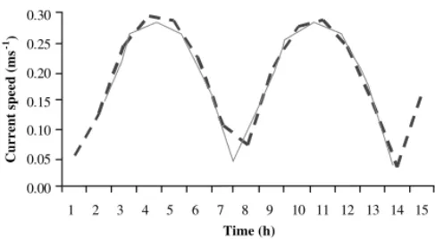
struc-tures on current flow and direction.Fig. 6 illustrates
a comparison under the 1993–1994 scenario between current speed measurements and model results at sam-pling point 14. There is a close agreement between predicted and observed data. A further comparison is illustrated under the 1999–2000 scenario for two measurements at sampling point 14, one inside the northern-most aquaculture area and the other outside
of that area in the navigation channel (Fig. 7). There
is a reasonable similarity between predicted and ob-served values. Confirming this, the slopes of the
0.00 0.05 0.10 0.15 0.20 0.25 0.30
1 2 3 4 5 6 7 8 9 10 11 12 13 14 15 Time (h)
Current speed (ms
-1)
Fig. 6. Current speeds predicted by the model (broken line) and measured (solid line) at sampling point 15 (cf.Fig. 4) (data from
Zhao et al., 1996), under scenario I (cf.Table 6).
Model II regressions between predicted and observed
values were not S.D. from 1 and the y-intercepts
were not S.D. from 0 (P < 0.05). The lack of
cur-rent velocity data at other points of the bay prevented more comparisons. The difference between the cur-rent speeds inside and outside the aquaculture area may be as high as 50%, as is with the use of different Manning coefficients.
InFig. 8, vector plots are shown for the 1993–1994 and 1999–2000 scenarios, showing the major patterns of current circulation in Sungo Bay. There is a domi-nant gyre circulation, with higher current speeds near the mouth of the bay. During high water, the gyre is counter-clockwise, whereas during low tide there is a clockwise circulation.
Simulations were also carried out assuming a con-stant Manning coefficient of 0.03, to compare with
the results obtained byGrant and Bacher (2001). The
average current speed obtained over the whole bay for
a 4-day simulation was 0.12 m s−1, with a maximum
of 0.59 m s−1. With the two different Manning
coef-ficients, an average of 0.06 m s−1 was obtained, with
a maximum of 0.46 m s−1. This represents a 50%
de-crease in average current speed, caused by inde-creased drag due to aquaculture structures, and shows the importance of having experimental estimates of the Manning coefficient. It is worth noting that the
max-imum values obtained by Grant and Bacher (2001)
both with constant (0.03) and variable Manning co-efficients (0.03 or 0.15) were a bit lower (0.5 and
0.3 m s−1) than those obtained in the present work.
However, the results are not fully comparable, due to the different distribution of aquaculture during our re-spective studies. In addition, the Aquadyn (Hydrosoft
Energy; seehttp://www.hydrosoftenergie.com) model
used byGrant and Bacher (2001)is based on a finite
element integration scheme, whereas the model used in the present study is based on a finite difference scheme. In spite of these differences, the predicted circulation patterns are quite similar. Another com-parison was made with the three-dimensional
hydro-dynamic model ofWan (2001), showing very similar
current patterns and current speeds.
3.1.2. Water temperature
Observed and predicted temperatures are shown in
Inside aquaculture area
0.00 0.02 0.04 0.06 0.08 0.10 0.12 0.14 0.16
1 3 5 7 9 11 13 15 17 19 21 23 25 27 29 31 33 35 37 39 41 43 45 47 49 51 53 55 57
Time (hours)
Current speed (ms
-1)
Model Observed
Circulation channel
0.00 0.05 0.10 0.15 0.20 0.25
1 3 5 7 9 11 13 15 17 19 21 23 25 27 29 31 33 35 37 39 41 43 45 47 49 51 53 55 57
Time (hours)
Current speed (ms
-1 )
Model Observed
Navigation channel
Fig. 8. Vector plots obtained with the model for the scenarios I and IIa (cf.Table 6) during low (LW) and high tides (HW) (referSection 2). Maximum current speeds indicated close to each scenario.
with minimum values around 2◦C during winter and
maximum values around 25◦C during August and
September. The slope of the Model II regression be-tween predicted and measured values was not
signif-icantly different from 1 and the y-intercept was not
S.D. from 0 (P <0.05).
3.1.3. DIN
DIN observed over several years (1983–1984, 1989–1990 and 1993–1994) is compared with model
predictions under the 1993–1994 scenario inFig. 10.
Due to several data gaps during the 1993–1994 pe-riod, the boundary condition for DIN had to be av-eraged using measures obtained over several years. This limited the effectiveness of our model
calibra-tion. Nevertheless, model results are in general well within the range of observed values. It is difficult to identify clear temporal patterns, since during different years, maximum and minimum DIN values occurred in different seasons. However, in general, higher val-ues occurred later in the year as are predicted by the model. With respect to the 1999–2000 period, too many nitrate values were missing to allow any rea-sonable comparison between observations and model predictions.
3.1.4. Phytoplankton
Chlorophyll concentrations observed are compared with model predictions under the 1993–1994 and the
93-94 99-00
St 2
0.0 5.0 10.0 15.0 20.0 25.0 30.0
Time (days)
Temperature (
ºC)
0.0 5.0 10.0 15.0 20.0 25.0 30.0
Temperature (
ºC)
0.0 5.0 10.0 15.0 20.0 25.0 30.0
Temperature (
ºC)
0.0 5.0 10.0 15.0 20.0 25.0 30.0
Temperature (
ºC)
0.0 5.0 10.0 15.0 20.0 25.0 30.0
Temperature (
ºC)
0.0 5.0 10.0 15.0 20.0 25.0 30.0
Temperature (
ºC)
83/84 89/90 Predicted 93/94
St 7
83/84 89/90 Predicted 93/94
Time (days)
9 9/ 00 P r e d i c t e d
St 16
St 10
83/84 89/90 Predicted 93/94
St 19 S t 20 St 16
St 20
St 19
1 31 61 91 121 151 181 211 241 271 301 331 361
Time (days)
1 31 61 91 121 151 181 211 241 271 301 331 361
Time (days)
1 31 61 91 121 151 181 211 241 271 301 331 361
Time (days)
1 31 61 91 121 151 181 211 241 271 301 331 361
Time (days)
1 31 61 91 121 151 181 211 241 271 301 331 361
1 31 61 91 121 151 181 211 241 271 301 331 361
9 9/ 00 P r e d i c t e d
9 9/ 00 P r e d i c t e d
Fig. 9. Observed and predicted temperatures at some of the stations depicted inFig. 4, for the scenarios I and IIa (cf.Table 6). Left charts correspond to scenario I and right charts to scenario IIa. From top to bottom, results correspond to stations at decreasing distances from the sea.
model predictions are well within the range of ob-served values. Again, as in the case of DIN, model cal-ibration was complicated by several data gaps during the 1993–1994 period, such that the boundary
St 2 0.0 10.0 20.0 30.0 40.0 50.0 60.0
1 31 61 91 121 151 181 211 241 271 301 331 361
Time (days) DI N ( mo l N l -1) 83/84 89/90 93/94 Predicted St 4 0.0 5.0 10.0 15.0 20.0 25.0 30.0
1 31 61 91 121 151 181 211 241 271 301 331 361
Time (days) DI N ( m o lNl -1) 83/84 89/90 93/94 Predicted St 7 0.0 5.0 10.0 15.0 20.0 25.0 30.0 35.0
1 31 61 91 121 151 181 211 241 271 301 331 361
Time (days) DI N ( mo l N l -1) 83/84 89/90 93/94 Predicted St 10 0.0 2.0 4.0 6.0 8.0 10.0 12.0 14.0
1 31 61 91 121 151 181 211 241 271 301 331 361
Time (days) DI N ( mo l N l -1) 83/84 89/90 93/94 Predicted St 13 0.0 1.0 2.0 3.0 4.0 5.0 6.0 7.0 8.0 9.0 10.0
1 31 61 91 121 151 181 211 241 271 301 331 361
Time (days) DI N ( m o lNl -1) 83/84 89/90 Predicted
Fig. 10. Scenario I (cf.Table 6): observed and predicted DIN concentrations at some of the stations depicted inFig. 4. From top to bottom, results correspond to stations at decreasing distances from the sea.
occurred in different seasons. Nevertheless, the model predicts two main maxima, one at the end of winter and the other during summer. The latter reflects a
sim-ilar peak in the boundary condition (Fig. 5). The
for-mer appears associated with a seasonal reprieve from light and/or temperature limitations. Comparison of model outputs indicates that throughout this period, phytoplankton was not limited by nutrients.
Model predictions for the scenario IIa are generally
within the range of observed values (Fig. 11). Two
93-94 99-00 St 2 0.0 2.0 4.0 6.0 8.0 10.0 12.0 14.0 16.0 18.0 20.0
1 31 61 91 121 151 181 211 241 271 301 331 361 1 31 61 91 121 151 181 211 241 271 301 331 361
Time (days) Chl ( m g l -1) 83/84 89/90 93/94 Predicted St 7 0.0 0.5 1.0 1.5 2.0 2.5 3.0 3.5 4.0 Chl ( m g l -1) 83/84 89/90 93/94 Predicted St 10 0.0 0.5 1.0 1.5 2.0 2.5 3.0 3.5 4.0 4.5 Chl ( m g l -1) 83/84 89/90 93/94 Predicted 0.0 1.0 2.0 3.0 4.0 5.0 6.0 Time (days)
1 31 61 91 121 151 181 211 241 271 301 331 361 1 31 61 91 121 151 181 211 241 271 301 331 361
Time (days) Time (days)
1 31 61 91 121 151 181 211 241 271 301 331 361 1 31 61 91 121 151 181 211 241 271 301 331 361
Time (days) Time (days)
Chl ( m g l -1) 99/00 Modelo St 16 0.0 0.5 1.0 1.5 2.0 2.5 3.0 3.5 4.0 Ch l ( mg l -1) 99/00 Modelo St 20 0.0 0.5 1.0 1.5 2.0 2.5 Chl (mg l -1) 99/00 Modelo St 19
Fig. 11. Observed and predicted chlorophyll concentrations at some of the stations depicted in Fig. 4, for the scenarios I and IIa (cf.
Table 6). Left charts correspond to scenario I and right charts to scenario IIa. From top to bottom, results correspond to stations at
decreasing distances from the sea.
values was S.D. from 0, whereas they-intercept was
not S.D. from 0 (P <0.05). The variance explained
by the model was significant (P <0.01). However, the
slope was significantly lower than 1 (P >0.05). These
results imply that the model explains a significant pro-portion of the observed variance, but the differences between model and observations are proportional to
0.0 100.0 200.0 300.0 400.0 500.0 600.0 700.0
1 31 61 91 121 151 181 211 241 271 301 331 361 Time (days) Zo o p la n k to n (m g F W m -3) St 2 0.0 50.0 100.0 150.0 200.0 250.0 300.0 350.0 400.0
1 31 61 91 121 151 181 211 241 271 301 331 361 Time (days) Zo o p la n k to n (m g F W m -3) St 4 0.0 20.0 40.0 60.0 80.0 100.0 120.0 140.0 160.0
1 31 61 91 121 151 181 211 241 271 301 331 361 Time (days) Zo o p la n k to n (m g F W m -3)
St 7 St 10
0.0 50.0 100.0 150.0 200.0 250.0
1 31 61 91 121 151 181 211 241 271 301 331 361
Time (days) Z oop la n k ton (m g F W m -3) St 13 0.0 20.0 40.0 60.0 80.0 100.0 120.0 140.0 160.0 180.0 200.0
1 31 61 91 121 151 181 211 241 271 301 331 361 Time (days) Zo op la n k to n (m g F W m -3)
Fig. 12. Scenario I (cf.Table 6): observed (diamonds) and predicted (line) zooplankton concentrations at some of the stations depicted in
Fig. 4. From top to bottom, results correspond to stations at decreasing distances from the sea.
3.1.5. Zooplankton
Measured zooplankton concentrations are com-pared with model predictions during the 1993–1994
period in Fig. 12. With the exception of the most
inner station considered, the model results follow the expected patterns and are well within the range of ob-servations. Model predictions could not be compared with measurements during the 1999–2000 period, because zooplankton had been collected by sieving through different-sized nets.
3.1.6. TPM and POM
Measured concentrations of TPM and POM are compared with model predictions from scenarios I
and IIa inFig. 13. During the 1993–1994 period,
sam-ples were collected with intervals of more than one month, thus posing difficulties both in defining the boundary conditions and for calibrating the model.
WhilstFig. 13illustrates the high temporal
93-94
99-00
Observed TPM Observed POM St 1 0.0 5.0 10.0 15.0 20.0 25.0 30.0 35.0 40.01 31 61 91 121 151 181 211 241 271 301 331 361
Time (days) 0.0 1.0 2.0 3.0 4.0 5.0 6.0 7.0 8.0 9.0 St 9 0.0 5.0 10.0 15.0 20.0 25.0 30.0
1 31 61 91 121 151 181 211 241 271 301 331 361
0.0 1.0 2.0 3.0 4.0 5.0 6.0 7.0 8.0 9.0 10.0 Observed TPM Observed POM Observed TPM Observed POM St 6 0.0 10.0 20.0 30.0 40.0 50.0 60.0 70.0 80.0
1 31 61 91 121 151 181 211 241 271 301 331 361
0.0 1.0 2.0 3.0 4.0 5.0 6.0 7.0 8.0 0.0 5.0 10.0 15.0 20.0 25.0 30.0 35.0
1 31 61 91 121 151 181 211 241 271 301 331 361
Time (days)
Time (days) Time (days)
0.0 1.0 2.0 3.0 4.0 5.0 6.0 7.0 8.0 9.0
St 16 Observed TPM
Observed POM 0.0 5.0 10.0 15.0 20.0 25.0 30.0 35.0 40.0
1 31 61 91 121 151 181 211 241 271 301 331 361
1 31 61 91 121 151 181 211 241 271 301 331 361 0.0 2.0 4.0 6.0 8.0 10.0 12.0 14.0 16.0 18.0 20.0 Observed TPM Observed POM Observed TPM Observed POM 0. 0 20.0 40.0 60.0 80.0 100. 0 120. 0 0. 0 2. 0 4. 0 6. 0 8. 0 10.0 12.0 Predicted TPM Predicted TPM Predicted TPM Predicted TPM Predicted TPM Predicted TPM Predicted POM Predicted POM Predicted POM Predicted POM Predicted POM Predicted POM Predicted POM St 19 St 16 St 20
Fig. 13. Observed and predicted TPM and POM concentrations at some of the stations depicted in Fig. 4, for the scenarios I and IIa
(cf.Table 6). Left charts correspond to scenario I and right charts to scenario IIa. From top to bottom, results correspond to stations at
decreasing distances from the sea.
Comparing observations and predictions for sce-nario IIa, the model underestimated TPM at station 16 (Fig. 13). Station 16 was that closest to the inner shore of the bay. There is reasonable agreement be-tween predicted and measured concentrations of TPM
at the other sampling stations. Model predictions and observations were also in reasonable agreement for
POM, except for the innermost station (Fig. 13). The
Table 7
Harvest (103tons DW for the kelps and FW for the bivalves) predicted under the 1993–1994 and the 1999–2000 aquaculture scenarios
Aquaculture scenarios Kelps Scallops Oysters
Expected value Predicted Expected range Predicted Expected range Predicted
I 93-94 40 40 43–60 55 13–24 21
IIa 99-00 28 25 10–19 9 34–46 42
IIb 99-00 (1/2)× – 25 – 8 – 26
IIc 99-00 2× – 25 – 0.6 – 58
IId 99-00 3× – 25 – 0.9 – 25
IIe 99-00 1×scallops, 2×oysters – 25 – 1.8 – 76
III 99-00 mixed scallop–kelp culture – 25 – 33 – 42
For the latter, results are given for decreased (1/2), normal and increased (two- and three-fold) bivalve densities, including for a new scenario with mixed scallop–kelp culture. Expected ranges are given when available (cf.Sections 2 and 2.3,Table 1andFig. 3).
they-intercept was not S.D. from 0 (P <0.05). The
variance explained by the model was significant (P <
0.0001). However, the slope was significantly higher
than 1 (P >0.05). These results imply that the model
explains a significant proportion of the observed vari-ance, but the differences between model and obser-vations are proportional to the TPM concentration (Mesplé et al., 1996). Regarding POM, similar results were obtained but only after excluding station 16 re-sults from the calculations.
0 10 20 30 40 50 60 70
1/2 X Standard 2 X 3 X
Seeding density
Harvest yield for the oysters (MTFW)
0 1 2 3 4 5 6 7 8 9 10
Harvest yield for the scallops (MTFW)
Oysters Scallops
Fig. 14. 1999–2000 scenario: harvest yields as a function of seed density (referSection 2).
3.1.7. Bivalves and kelps
Data describing scallop growth were used to cali-brate an ecophysiological model with time series of measured chlorophyll, TPM, POM and temperature (Hawkins et al., 2002). A lack of data prevented similar calibration for oysters cultured in Sango Bay. Instead,
parameters reported byBarillé et al. (1997)were used.
Simulated harvest yields of kelp, scallop and
oys-ter are summarised for scenario I inTable 7.
The lower limits of these ranges are based on official estimates, whereas upper limits are based on known densities, including the size of each harvested species and available mortality data. Both of these limits may be subject to large errors.
Simulated harvest yields during scenario IIa are
summarised in Table 7and inFig. 14. Model
predic-tions are broadly within the expected ranges, albeit for scallops marginally below the lower limit of
esti-mated harvest (Table 7). In possible explanation, the
1999–2000 prediction for scallops was obtained as-suming 4.5 cm as the minimum harvest size, as they did not quite reach the official 5 cm during the normal harvest season.
Compared with scenario I, the decrease in kelp production under scenario IIa resulted from the lower initial standing stock, whereas the increase in oyster production may be explained partly by the higher
initial standing stock (cf. Section 2.3). The decrease
in scallop production under scenario IIa, in spite of the higher initial standing stock in scenario I (cf.
Section 2.3), resulted from the shorter rearing period and harvest size.
Fig. 15. Water residence times (days) at different parts of the bay, estimated from the time it takes for the sea water to replace the water inside the bay under the current culture Scenario IIa (refer text).
3.2. Sungo Bay carrying capacity for bivalve culture
One of the simplest ways to assess potential effects of bivalve culture at the ecosystem scale is by compar-ing the time scales of water renewal, phytoplankton doubling and particle clearance by bivalves, thereby estimating the time it takes for a particular standing stock of bivalves to filter all water within the system (Dame and Prins, 1998).
Water residence time in Sungo Bay was estimated by initialising the model domain with zero salinities,
assuming 35‰salinity at the sea boundaries and
run-ning the model until salinity reached 35‰ over the
whole grid. It took up to approximately 20 days be-fore the bay was completely replaced with seawater (Fig. 15), which was well within the range estimated
for other systems (Table 8). The model also predicted
an average concentration of 1.5 mg m−3 chlorophyll
throughout Sungo Bay over a year (combined average of scenarios I and IIa), and which was lower than re-ported for other main cultivation sites, although sim-ilar to that observed in the Ria Formosa, Portugal
P
.
Duarte
et
al.
/Ecolo
gical
Modelling
168
(2003)
109–143
Table 8
Physical characteristics, phytoplankton production and bivalve grazer parameters of some coastal ecosystems (adapted fromDame and Prins, 1998andFalcão et al., 2000) (see text)
System Area
(km2) Depth(m) Volume(
×106m3)
Residence time (day)
Average annual concentration (mg m−3)
Primary production
(×106g C per day) Cell doublingtime (day) Totalbiomass
(×106g)
Bivalve clearance time (day)
Sylt 5.6 1.3 7 0.5 3.0 0.9 0.8 84 4.0
North Inlet 8.8 2.5 22 1.0 7.0 6.2 0.8 338 0.7
Carlingford Lough 39.5 5.0 196 65.8 3.2 1.3 16.9 14 490.2
Marennes-Ol´eron 135.7 5.0 675 7.1 13.0 22.2 10.0 2850 2.7
South San Francisco Bay 490.0 5.1 2500 11.1 2.6 196.0 1.1 6255 0.7
Narragansett Bay 328.0 8.3 2724 26.0 3.0 243.0 1.7 1267 25.0
Osterschelde 351.0 7.8 2740 40.0 7.5 200.0 3.1 8509 3.7
Western Wadden Sea 1386.0 2.9 4020 10.0 8.0 994.0 1.0 14700 5.8
Ria de Arosa 228.0 19.0 4335 23.0 16.0 172.7 0.6 6900 12.4
Delaware Bay 1942.0 10.0 19420 97.0 9.9 777.0 7.4 178 1278.0
Cheasapeake Bay 11500.0 7.0 27300 22.0 6.9 6006.0 0.9 1900 325.0
Ria Formosa 105.0 1.5 155 1.0 1.4 3.1 1.6 7000 4.0
(Table 8). Despite low chlorophyll concentrations,
av-erage total primary production of 26.5×10⁶g C per
day and the average cell doubling time of 5 days were higher and faster, respectively, than for some of the
other ecosystems (Table 8). This was in part due to the
relative transparency of water, with an average light
extinction coefficient of 0.5 m−1(Gazeau and Bacher,
unpublished).
The total biomass of bivalve shellfish in Sungo Bay was estimated from known yields. Bivalve clearance time was calculated assuming that the average clear-ance rate for a commercial sized scallop of between
5 and 6 cm shell length was 2.5 l h−1(Hawkins et al.,
2002), and that the average clearance rate of a
com-mercial sized oyster of 7 cm shell length was 4 l h−1
(Barillé et al., 1997). Average clearance rates were multiplied by the number of individuals at marketable
size, that were 1.2×10⁹scallops and 107 million
oys-ters, calculated from total biomass figures. The result-ing time estimated for suspension-feedresult-ing bivalves to filter all water within the system averaged 10.1 days, which is about half the estimated average residence
time for water renewal (Table 8). Cultured bivalves
therefore depend on food made available within Sungo Bay, from sources that may include benthic resuspen-sion and/or primary production. Indeed, the estimated average cell doubling time of only 5 days confirms
this (Table 8).
It might be hypothesised, given that phytoplankton doubles its biomass in approximately half the time it takes bivalves to clear all water in the bay, that Sungo Bay is being exploited below its environmental carry-ing capacity, and that bivalve standcarry-ing stock could be increased substantially. However, as will be discussed below, this assumes that local food depletion is not important, and that carrying capacity will not be af-fected by the way bivalves are distributed within the bay. The problem becomes even more complex when species interactions are considered.
Simulated harvest yields during scenario II, for different bivalve seeding densities that included a range from half to three times those currently
em-ployed, are summarised and illustrated inTable 7and
in Fig. 14, respectively. The model predicts a sharp decrease in scallop production when stock density is increased above the current value, and in oyster production when stock density is more than twice the current value. Average annual chlorophyll
concen-Table 9
Annual mean concentrations of chlorophyll, total particulate matter (TPM) and particulate organic matter (POM) predicted by the model under the 1993–1994 (I) and the 1999–2000 aquaculture simulations IIa, IIb, IIc and IId (cf.Sections 2 and 2.3,Table 6
andFig. 3)
1993–1994 1999–2000
I IIa IIb IIc IId
Chlorophyll (g l−1) 1.4 1.5 2.0 1.0 0.8
TPM (mg l−1) 19.6 14.9 15.1 14.6 14.5
POM (mg l−1) 3.5 2.4 2.6 2.1 2.0
trations predicted throughout Sungo Bay declined by almost 50% as stock increased by three times from the current culture practice under scenario IIa to hy-pothetical scenario IId, although with proportionally
smaller reductions for TPM and POM (Table 9).
These results suggest that Sungo Bay is already being exploited close to the environmental carrying capacity for scallop production at the present aqua-culture scenario, whereas there may be some potential for increased oyster production. Any significant in-crease in yield must to a great extent depend upon the relative spatial distribution of cultivated species.
The effects illustrated inFig. 14follow the expected
parabolic response (Bacher et al., 1998). For both
scal-lops and oysters, initial increases in harvest yields are proportionately less than expected with the doubling in stock densities, indicating growth limitation at even half the current densities. Above a certain threshold, both food limitation and reduced growth rates result in a reduction in harvest yield, when cultured species may not reach their commercial size in time for nor-mal harvest. Under such conditions, it is conceivable that total yield may be higher at larger temporal scales
than were analysed here (cf.Ferreira et al., 1998). This
could happen if a large number of cultured bivalves reach harvestable size in more than 1 year. However, such considerations may be compromised by uncer-tainties concerning age-dependent mortality. In any case, because mass mortalities of scallops occur dur-ing summer in Sungo Bay, cultivation strategy needs to be directed towards a rearing period of less than 1 year, as at present.