1
DETERMINANTS OF EXPORT DIVERSIFICATION AND
SOPHISTICATION IN SUB-SAHARAN AFRICA
1Manuel Herédia Caldeira Cabral (University of Minho, NIPE) Paula Veiga (University of Minho, NIMA)
July, 2010.
Abstract
This paper studies the political and economic factors that determine successful export diversification (ED) and export sophistication (ES) strategies in the Sub-Saharan African (SSA) countries and also the way in which successful ED and sophistication strategies contribute to explain the improving in some of the millennium development goals (MDG). We run separate regressions for the determinants of ES and ED, using disaggregated data of the 48 SSA countries, from 1960 to 2005. The results suggest that better governance is an important determinant for the success of diversification and sophistication strategies in SSA. In particular the level of corruption, transparency and accountability are important factors in limiting or promoting the scope of diversification and the level of sophistication of the exports. The results also suggest that increases in human capital in SSA countries promote both ED and ES, showing that the level of education of the workforce is positively related with ES and ED, with higher levels of education (tertiary) playing a more important role in explaining ES, while lower levels of education (primary) being more important as determinants of ED. In the second part we explore the links between ED and ES and growth presenting evidence that ED and ES are linked to growth stability in SSA. This study also suggests that the Sub-Saharan countries that were more successful in achieving ED and ES tend to be more successful in improving the living conditions of their population. Using different variables of Infant Mortality (one of the MDG) and life expectancy as dependent variables, we present evidence that suggests that in SSA higher ED and ES are associated with lower infant mortality and higher life expectancy. We show that this result is robust, presenting positive and significant results even when a large number of different control variables are introduced, or when fixed effects and instrumental variables are considered. The evidence suggests that ED and ES are part of the solution for a successful development of SSA.
1
2 1 - INTRODUCTION
This paper aims to answer two questions: First, what are the main political and economic determinants of successful export diversification (ED) and export sophistication (ES) strategies for Sub-Saharan African (SSA) countries? Second, are ED and ES linked to economic growth, growth stability and to the ability to pursue the millennium development goals?
These are important issues , since overall SSA economies exhibit very low levels of ED and ES. .Most of SSA economies have been unable to follow a sustainable path towards increasing exports diversification and sophistication. Their experiences differ from those of Asian developing countries. Over the past decades, Asian developing countries have been increasing their competiveness and, at same time, have been more successful both at diversifying and improving the sophistication of their exports.
Increasing the ED level is critical for SSA economies, since a high degree of concentration of resources in a few sectors increases the risks associated with external shocks (see Kalemli-Ozcan et al. 2003). The consequences can be particularly serious in cases where the core sectors of the economy are based in commodities with volatile prices, which is the case of the majority of SSA countries. ED strategies can take place in different forms and dimensions but are likely to involve moving into products of higher quality (Schott, 2004) or expanding into new markets (Brenton and Newfarmer, 2009).
In the present study we explore the role that institutional and political variables can play in promoting ED and ES in SSA countries. We believe that this is one of the important contributions of this study, since the role of institutional variables was has not been widely studied in the empirical literature. Few studies, namely by Klinger and Lederman (2004, 2006) and more recently by Parteka and Tamberi (2008) have addressed these issues2. In fact, most previous ED studies focus mainly on the empirical link between the level of diversification and the level of development (the ‘specialisation curve’)3.
2
Moreover none of these studies use data from African countries, in which we expect that institutional factor play an important role in constraining the scope for diversification.
3 Imbs and Wacziarg (2003), Cadot et al. (2007), Koren and Tenreyro (2007) found a reversal in the
3 Another important contribution of the present study is to provide evidence that ED and ES can contribute to economic growth and stability as well as to improve well-being in SSA countries. Although several previous studies have discussed how per capita income may contribute to ED, there is still only limited evidence on the impact that ED and ES can have on growth and development, particularly in SSA countries. An exception is the recent study by Matthee and Naudé (2008). The authors analyze export diversification across South Africa’s regions. Using export data from sub-national districts, the authors found that regions with lower level of export specialisation and more diversified exports tended to experience higher economic growth rates, and contributed more to South Africa overall exports.
There is also limited evidence linking ED and ES to income stability. Although one can find several references in the development literature blaming export concentration for growth instability, few studies have directly addressed this issue. Here we study how ED and ES contribute to growth and stability in the SSA and also how these contribute to improve the levels of development. The paper uses infant mortality and life expectancy as development indicators.
Our approach differs from the trade and development literature. Instead of focus on understanding how trade openness contributes to foster economic growth, this study is concerned with how different forms of involvement in international trade can contribute to increase growth and social conditions in SSA countries. The goal is to assess how different patterns of involvement in world trade (namely more or less diversified export structure or greater sophistication of exports) might contribute to growth and stability but also to a more balanced development, and in this way contribute to increase life expectancy or reduce infant mortality.
A basic raw data analysis (section 2) suggests that more diversified or/and sophisticated exports may have an independent contribution for development and improvements in the quality of life and health status of the populations. Data suggests that ED and ES may contribute to spread development across regions and social groups of countries which can contribute for social development. For this reason, we will focus
4 directly in development variables instead of studying only the effects of ED and ES in increasing the exports or in the GDP growth.
The paper is organized as following: In Section 2 we present the raw data and discuss the hypothesis that data analysis suggest. Section 3 presents the data sources, the variables and econometric methods used in the regressions of sections 4 and 5. The regressions presented in section 4 consider ED and ES as dependent variables and try to access the determinants that explain the variation of ED and ES across the 48 SSA countries from 1960 to 2005 (45 years). This allows us to determine the factors that promote and inhibited ED and ES in SSA. We use two major variables to measure trade diversification (the Herfindhal index and the Theil index) and one variable to measure ES (the EXPY index)4.In section 5 we discuss why ED and ES are important for SSA. There we ask if ED and sophistication promote growth and stability in SSA, and contribute to improve life expectancy and to reduce infant mortality. Section 6 concludes.
2 - MOTIVATION
Graph 1 shows the evolution of the average number equivalent in the 48 SSA and in the Other Middle Income and Developing (MID) countries. A high concentration of exports in a limited number of products is a well known problem in virtually all developing countries but it is even more accentuated in the SSA countries. As the data clear shows, on average, SSA countries exhibit a lower level of export diversification than the other developing countries. Moreover, ED has been increased, on average, at a much slower pace in SSA countries than in other developing countries. Since the 1960´s, ED increased in a marked way in the developing countries, particularly in those countries that have improved their level of development, which contrast with the stagnation experienced in SSA.
4
5 Graph 1 here
Graph 2 here
Graph 2 presents the evolution of the GDP per capita in the SSA countries as well as in the other middle income and developing countries in the sample. The evidence, presented for the GDP per capita, is similar to that obtained for ED. The parallel between lower ED and lower increase in GDP per capita in SSA countries, when compared with the other developing countries, serves as motivation for the econometric work developed in the next section. The evidence suggests that a low level of ED is a part of the marginalization of Africa in international trade, and has been induced by this marginalization phenomenon.
Graph 3 presents the evolution of ES in SSA and MID countries over the last decades. It is evident from the graph that ES is lower in SSA countries than in the other MID countries. Nevertheless, the evidence suggests that there has been some improvement in the average level of sophistication in the recent years, although this progress is still unstable. The important evolution of ES in Asian countries during the recent years shows that developing countries can upgrade their level of sophistication.
Graph 3 here Graph 4 here
Graph 4 plots the average number of NE of each country against its average GDP per capita. The evidence suggests that the positive relationship between the GDP per capita and ED found in previous studies can also be confirmed in a SSA sample. The graph for ES (not shown) presents similar evidence and also suggests a positive relationship between ES and GDP per capita exists in the SSA countries.
6 are similar to those obtained with ES (Graph 7). The evidence presented concerns only SSA countries, but a similar distribution was found when all the 143 developing countries in our sample were included.
Graph 5 here Graph 6 here Graph 7 here
This evidence should be taken with care. The positive relationship may reflect the effects of other variables. To draw stronger conclusions a more solid econometric work has been done ( see section 5).
3 – REGRESSIONS, DATA AND VARIABLES
3.1 – Econometric Methods
In the present study we estimate two general types of equations. The first uses the ED and ES indexes as dependent variables. The aim is to investigate which factors (determinants) inhibit or promote ED and ES. The results of these equations are presented and discussed in section 4. The second type of equations tries to explore the contribution of ED and ES variables for selected development goals. The equations presented in section 5 uses ED and ES as independent variables in GDP Growth, Growth variance, Infant Mortality, and Life expectancy regressions.
7 The general formulation of the first type of equations is:
lnEDit = A+ B2lnPOPit+B3lnYPCit+B4(OTHERit)+B5(INSTit) lnESit = A+ B2lnPOPit+B3lnYPCit+B4(OTHERit) + B5(INSTit)
Where the dependent variables EDit and ESit are respectively the ED and the ES indexes of country “i” in the year “t”.
The explanatory variables reflect an eclectic approach, where the economic variables (such as level of development, endowments, size of the economy, and education of the work force) are used simultaneously with geographic variables (such as distance or those reflecting a landlocked country) and institutional variables for each country (such as governance, control of corruption, education spending, etc).
Previous studies present evidence that ED is correlated with income, and that higher levels of ED are associated with higher long-run growth. The literature about ES also suggests that ES promotes faster growth. We replicate these results for SSA, but using a different approach. Our study focus mainly how different forms of international trade involvement contribute to improve the level of development of the SSA countries.
8 development and in this way give a stronger contribute to improve some of the development goals, than the mere effects of increase in exports or in the GDP growth.
Once more it is particularly interesting to link the trade variables to the institutional ones to study the empirical links between more diversified and more sophisticated export structures and development indicators. This allows us to assess the role of ED and ES in promoting a successful and sustainable development in SSA.
So the second type of models will be given by the general form:
lnGROWTHit = A + B1(lnEDit) + B2(lnESit) + B3(lnOTHERit) lnVARGROWTHit = A + B1 (lnEDit) + B2(lnESit) + B3(lnOTHERit)
lnINFANTMit = A + B1(lnYPCit) + B2(lnEDit) + B3(lnESit) + B4(lnOTHERit) lnLIFEit = A + B1(lnYPCit) + B2(lnEDit) + B3(lnESit) + B3(lnOTHERit)
Where the dependent variables are different measures of the different development goals (life expectancy, infant mortality5), and the explanatory variables will include the level of development (YPC), export diversification (ED) and export sophistication (ES), and other control variables, which include trade policy, institutional, and other economic and geographic variables. The variables are described in Table B in annex.
The results presented are for log-log model which has a better fit than the linear regression or other specifications tried. We also estimate robust standard errors to correct for heteroskedasticiy. The robustness of the results were tested by considering a Fixed Effects instrumental variable approaches to deal with potential omitted variable and the endogeneity of the ES and ED variables 6.
5 We also considered mortality rate of children under five years old 6
9 3.2 – DATA AND VARIABLES
The data used came mainly from the OCDE SITC trade data and from the World Bank tables. Table B in appendix presents a short description of the variables and its sources. Here we describe in more detail the most important variables, in particular those of ED and ES.
3.2.1 - Trade Variables
a) Herfindahl Index and Number Equivalent
The Herfindahl Index is given by:
In which si is the share of each product in total exports of each country (si = Xi/∑ Xi), with Xi being the exports of each good “i” of each country “j” in year “t”. The Herfindhal index is a concentration index. Instead of using this directly we use the Number Equivalent proposed by the same author, which is a diversification index:
Number Equivalent = ED = 1/H b) Theil Index
10 In which the xi are the exports of each product, and the average value of the exports of each product is given by:
In which N is the total number of products. If the exports are divided in a even way by all the product categories this index will be zero, if on the contrary these are all concentrated in one single category then the maximum value will be obtained, a value of ln (N)
c) EXPY and PRODY indexes.
11 4 – DETERMINANTS OF EXPORT DIVERSIFICATION AND SOPHISTICATION IN SUB-SAHARAN AFRICA
4.1 – THE EFFECTS OF GEOGRAPHY, LEVEL OF DEVELOPMENT AND ENDOWMENT VARIABLES
The first step in the study is to estimate a model based on previous ED studies. This “standard” model, that will be use as a benchmark, includes as independent variables the level of development (YPC – GDP per capita), the size of the country (POP7), endowments (OIL and LANDPC) as well as geographic characteristics, such as being a landlocked country (LANDLOCK). Then, we will add several variables to the model. This exercise will allow us to evaluate the role of different political and institutional variables in explaining ED and ES.
The per capita income (YPC) variable has been used in a large number of studies focusing on the specialization curve question (Imbs and Wacziarg, 2003; De Benedictis et al., 2009; Parteka, 2007; Cadot et al., 2007 and Koren and Tenreyro, 2007)8. The evidence suggests that, in developing countries, there is a monotonic increasing relationship between the level of development and the export diversification. This is consistent with theoretical contributions that stress the limited diversification opportunities at lower levels of development, namely because of the scarcity of capital and the indivisibility of investment projects (e.g. Acemoglu and Zilibotti, 1997).
The size of the economy appears also to be an important determinant of ED level. The monopolistic competition models (Dixit and Norman, 1980; Krugman, 1981; Helpman and Krugman, 1985) argue that market size directly affects the degree of product differentiation, with bigger countries being able to produce wider range of goods, since there are scale economies. The size of economy was also considered in several
7
Alternatively, the GDP was also considered as a measure of economic size. The results were similar. We chosed the POP variable because the GDP variable raised multicolinearity problems in the regression when used simultaneously with YPC, affecting in some cases the significance of this variable (that was still validated at the 1% level in most cases, but when a large set of control variables was considered would became only significant at the 5% level).
8
12 previous empirical studies. (e.g. Hummels and Klenow, 2005; Parteka and Tamberi, 2008). Their results confirm a positive relation with ED.
The New Economic Geography models (Krugman and Venables, 1990, 1995; Amiti and Venables 2002; Venables and Limão 2002) suggest that transport costs and distance have an effect in the level of specialization of a country. According to the models, a lower distance to the main world markets, access to the sea and overall lower transport costs, determine the ease with which a country can increase the variety of products exported to the world markets.
Using a sample of developed and developing countries Parteka and Tamberi (2008) find that transport costs discourage ED. Matthee and Naudé (2008), using data from the regions of South Africa, found that domestic transport costs are inversely related to the degree of ED concluding that “most districts with high export diversity values are located within 100 km of the nearest port”. This evidence suggests that landlocked countries or areas distant from the sea face extra difficulties to diversify export. This is consistent with the evidence found in previous studies revealing that landlocked countries face higher transport costs and have lower trade volumes than coastal countries (Radelet and Sachs, 1998; Limão and Venables, 2001).
Trade liberalisation, in a context where economies of scale and transport costs play an important role, is also likely to affect product diversification (Krugman and Venables 1990, Haaland et al. 2002), with important gains from trade that can cause increases in product diversification (Costas et al. 2008). Nevertheless, the New Economic Geography models also stress that the decline in transaction costs brought by trade liberalization may decrease the diversity of production (and therefore, the export diversification) particularly in peripheral countries.
The abundance of natural endowments also is likely to limit the scope of diversification, and sophistication of the export structures, since countries abundant in one resource tend to have highly concentrated export structures (Harrigan and Zakrajsek, 2000). This problem is particularly important for the SSA countries since several of them are oil exporting countries or are largely dependent on few agriculture cash crops.
13 different levels of aggregation9, and alternative export concentration measures, namely the Theil index. Table 1 reports the results for ED regressions, using NE as a measure of ED.
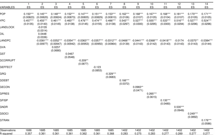
The signs of estimated coefficients in the “standard” model are consistent with those obtained in previous studies10. Together they explain almost 37% of the variation of the Number Equivalent (see Table 1). The results suggest that higher level of development (YPC) is associated with more diversified exports. According to the model estimates, everything else constant, a 10% increase in the level of development would result in a 2% increase in the number equivalent. This result confirms previous evidence that suggested a negative relation between export concentration and level of development for the case of developing countries. Our results also confirm that the size of the country (POP) is positively related to ED. The estimated coefficient suggests that a SSA country with double of the average population would have exports that are, on average, 15% to 25% more diversified than an average size country in the region.. The variables of the “standard” model were used also to explain the indexes of export sophistication (EXPY). Table 2 reports the results. The positive relation between ES and the level of development comes as no surprise. The results for the SSA sample confirm a positive and significant relationship between the YPC and the ES index, which suggests that the indexes developed by Haussman et al. (2005) can be applied to study the African case.
Perhaps, more interesting is the estimated relationship between the level of ES and the size of the economy (see table 2). The results suggest that the size of the economy is an important determinant of the level of ES, such that bigger economies tend to have more sophisticated exports. This result is valid when the model controls for the YPC and it is robust to the disaggregation of the data used to calculate the indexes of ES. The size
9 We calculated the ED and ES indexes (Herfindhal, Theil and EXPY) using data disaggregated in five
different levels, according to the categories of the SITC trade data (Rev2). In the rest of the work we only report the results using indexes calculated with the most disaggregated data, since they give a more accurate and detailed picture of country’s exports. In the case of the ES the more disaggregated indexes are also more rigorous since they reflect the level of sophistication of the exports in a more accurate way. In general, the results are similar independent of the level of disaggregation used. Nevertheless, the results tend to be less strong and more inaccurate when indexes when very aggregated data are used, namely when the 1 and 2 digit categories are chosen.
10
14 seems to have an even more pronounced effect in the sophistication of exports in the case of the SSA countries than other developing countries. This result suggests that the lack of dimension, the failure to sustain industries with more important internal and external economies of scale, and the inability to achieve the positive externalities of agglomeration of economic activity, might help to explain the limited progress in some African countries towards a more diversified and sophisticated structure of their exports. This is an interesting result that suggests that the efforts towards a regional integration, by increasing the economic size in which SSA firms can operate, might play an important role to successful ED and ES strategies
Although there are important similarities, the results clearly show that ES and ED are two different phenomena11. The variables LANDLOCK and OIL are not significant when used to explain ES, while are important determinants of ED. Only the availability of land-per-capita appears to affect both ED and ES. An interpretation of the capability of this variable in explaining ES is that it reflects a comparative advantage in exporting agricultural goods which is associated to lower levels of sophistication12.
4.2 – INSTITUTIONAL AND POLITICAL VARIABLES
An important hypothesis of our work is that institutional, political and governance variables play an important role to explain the ability of the SSA countries to successfully promote diversification and sophistication of their export structures. Therefore, we included in the regressions the governance variables, namely indicators of corruption, rule of law and political stability, and test how these explain ED and ES levels.
The evidence presented in Table 2 suggests that there are some differences in the determinants of ES and those of ED. The fact that a country is landlocked and/or exports oil does not seem to affect ES in a significant way (see Table 2- equation 2). In the case of ED, on other hand, these two variables appear to give an important contribution. On the other hand there are also similarities in the determinants of ED and ES. The size and
11
The ES indexes are very recent and there is no agreed set of determinants established in the literature.
12 In the sense that most of the countries specialized in exporting primary products are developing
15 level of income contributes to increase both ED and ES, while land abundance is associated with lower ED and ES.
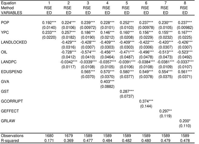
We considered 26 different governance and institutional variables. Given that these variables are likely to be strongly correlated, separate regressions will be run . The estimated coefficients for ED regressions are presented in Table A.1. Results suggest that in case of the ED, when the regressions include only a small set of control variables (only POP and YPC) 1913 out of the 26 coefficients were positive and statistically significant..This can be interpreted as evidence that better governance is associated with more ED. Nonetheless, when more control variables are included in the regressions14, several of the governance and institutional coefficients lose their statistical significance at conventional levels. Only six variables, appear to be robust15..Their estimated coefficients are positive and statistically significant even in a full model The results are very interesting. According to them improvements in government accountability (GVA), rule of law (GRLAW), political stability (GST), effectiveness (GEFFECT), and control of corruption (GCORRUPT), may contribute to expand the scope of products that a country is able to export.
The estimated coefficients suggest that the effects of better governance are of similar magnitude than those of increasing education spending and being in a landlocked country (with opposite sign). Moreover, the effects of better governance appear to be bigger that the marginal effect of economy size and level of development. Another interesting result is that the environment sustainability rating presents a significant positive sign in all regressions explaining ED.
In what concerns the role of institutional and political determinants of export sophistication there are marked differences with the results obtained in the ED
13
Amongst the remaining 7, 3 obtained non-significant results, and other four present evidence contradictory with what was expected, with significant coefficients.
14
The extended equation included POP and YPC, along with four other variables: LANDLOCK, OIL, LANDPC and EDUSPEND.
15
16 regressions. Most of the six robust governance and institutional variables explaining ED are not statistical significant in ES regressions.
The evidence suggesting that governance and institutional factors affect the sophistication of the exports of the SSA countries is weaker. The majority of the institutional variables (15 out of 26) are not statistical significant at conventional levels of significance, even when the models control only for a small number of other variables16.. The results are difficult to interpret. They may be due to the limitations of the available governance indicators or due to the small variance of these variables within SSA countries sample17. The results reveal that the estimated coefficient in 7 governance and institutional variables are positive and significant, and in other two are negative and significant as well.
The variables that appear to impact positively the level of ES in SSA are “transparency, accountability and control of corruption in the public sector” (GTRAN), the “debt policy rating” (GDEBT), “economic management cluster average” (GECON), the “debt policy and the fiscal policy rating” (GFISP), “Policies for social inclusion” (GSOCI) and “gender equality” (GNDR). On other side the estimated coefficients for GCORRUPT, and (GRQ) are negative, suggesting a negative association between the level of control of the corruption and of regulatory quality and ES, which are difficult to interpret.
4.3 –EDUCATION AND QUALIFICATIONS
The level of qualifications of the workforce and the efforts made in education are expected to have an important impact on the capability of each country to diversify and upgrade the quality and sophistication of their exports. Recent intra-industry trade (IIT) models based on the vertical IIT tradition emphasize the role of the level of qualifications in promoting product differentiation (e.g. Gullstrand, 2000).
The role played by education and human capital quality in promoting ED or ES has not been fully explored in the literature. The recent study by Parketa and Tamberi (2008) is one of the few exceptions. The authors emphasise that higher quality of human
16 When only POP and YPC variables are considered as control variables. 17
17 capital facilitates the production diversification and increases the rate of new activities in the economy. The authors also claim that human capital affects export diversification, namely through product innovation.
In this paper we are concern with both aspects, that is the level of qualifications and the effort make in education. To capture the level of qualifications we use as variables the percentage of the labor force with at least primary education, secondary or a tertiary level of education. To capture the education efforts we use a variable on the share of GDP spent in education (EDUSPEND). Table 3 reports the estimated coefficients for education variables,
The results suggest that export diversification tends to increase with the share of GDP spent in education. The estimated coefficient on EDUSPEND is positive and statistically significant at conventional levels (see table 3). The governance variable reflecting building human resources index (GHRES) also obtains a significant and positive result, on ED regressions, although is less robust18.
This evidence suggests that improving the education standards of the labor force is determinant for a successful export diversification strategy in SSA countries19. Our results indicate, everything else constant, investments in lower levels of education have higher return in terms of ED. Indeed the results indicate that improving the lower levels of education has a stronger effect in promoting the diversification of the economy. On other hand the efforts in increasing the higher level of qualifications does not have a very clear effect on ED20.:the estimated coefficients are positive and statistically significant in the “standard” model but are not robust when more control variables are added. These conclusions have obvious and important policy implications
The results obtained for ES are different of those for ED. The estimated coefficients of EDUSPEND and building of human resources (GHRES) are not statistically significant at conventional levels, while those for variables on the percentage of population within each level of qualifications, suggest that higher levels of education are more important in explaining ES (see equations 9, 10 and 11 of table 3).
18
See table A1 in appendix. The coefficient of this variable became non significant when larger number of control variables were included.
19 See the results for the variables EDUPRIM, EDUSEC,EDUTER and EDUSPEND. 20
18 5 – EXPORT DIVERSIFICATION AND SOPHISTICATION AND GROWTH
AND DEVELOPMENT IN SUB-SAHARIAN AFRICA.
5.1 - DIVERSIFICATION, SOPHISTICATION, GROWTH AND INSTABILITY
The theory of endogenous growth suggests that export diversification may be favorable to development (Feenstra et al. 1999) and to the rate of economic growth. China and several other Asian economies are good examples of diversified economies with fast growing rates. Their results contrast with other areas such as SSA that combine slow growth and strong export concentration for long time. This evidence is consistent with several results in the literature that suggest that those developing countries that diversify their exports experienced faster growth (De Piñeres and Ferrantino, 1997; Herzer and Nowak-Lehnmann, 2006). Moreover, cross-country comparisons found that ED is positively associated with long-term rates of growth (e.g. Al-Marhubi, 2000; Funke and Ruhwedel, 2005). There is also evidence pointing out that an increase in export variety raises the productivity level of industries (Feenstra and Kee, 2008). In a recent study of Matthee and Naudé (2008) show that “Regions with less specialisation and more diversified exports generally experienced higher economic growth rates, and contributed more to overall exports from South Africa” - Matthee and Naudé (2008: 2).
19 et al., 1991). An increase in manufactured exports may also, in the context of SSA, contribute to increase the level of sophistication of their exports. Hausmann et al. (2007) argue that the composition of a country’s exports matters, since exporting more sophisticated and higher productivity goods may lead greater export performance and higher growth. An overall increase in the level of sophistication of the production may also presents externalities and spillovers. These externalities benefit other economic activities and improve the ability of more industries to compete internationally (Herzer and Nowak-Lehnmann, 2006).
Here we use the PRODY and EXPY indexes proposed by Hausmann, et al. (2007) to investigate how increasing sophistication can contribute to a higher growth and stability in SSA countries. Table 4 and 5 present the results of the estimations for the role of both ES and ED.
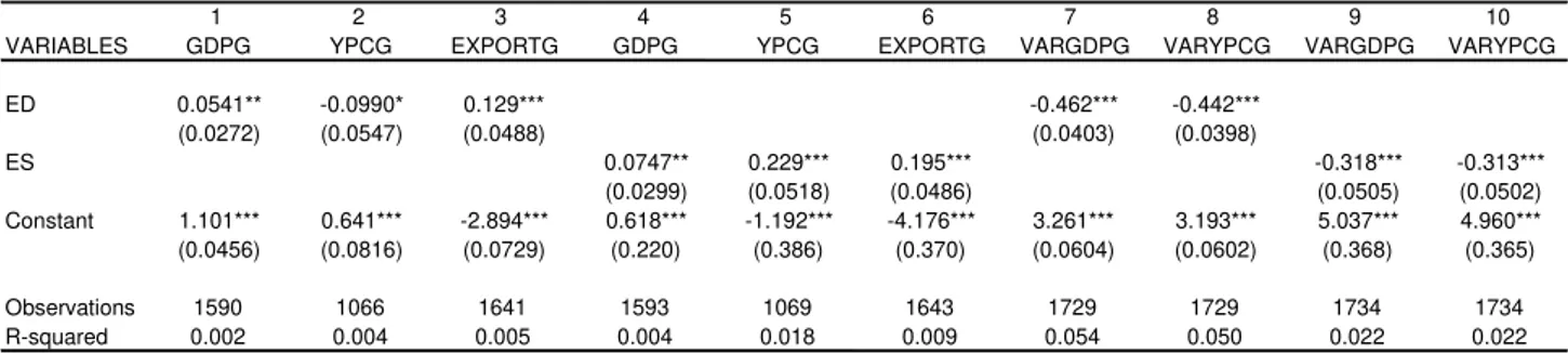
The results suggest that ED contributes to GDP and export growth in the SSA countries. Nevertheless, the coefficients of the export growth estimates are not robust. The estimated coefficient becomes not statistically significant when country fixed effects are introduced. Only in the GDP growth regressions, we find positive and significant coefficients for the ED variable both with and without fixed effects.
The OLS pooled regressions suggest a positive relation between ES and the rate of growth of GDP, YPC and Exports (Table 4). Nevertheless, in the country fixed effects model (Table 5), only the estimated coefficient on the export growth variable remains significant although only at the 10% level. One can also notice that the R2 of the first six equations are very low, so ED and ES seem to explain very little of the variance of the growth variables. In the end, these two variables are not very robust and are able to explain only a very low proportion of the total variance of the growth variables. These results lead us to conclude that the evidence fails to confirm a positive and robust relation between both ED and ES and growth in SSA countries.
20 in the rate of growth of both GDP and per capita income. These results remain robust when country fixed effects are considered.21
The estimated coefficients suggest that a 10% per cent increase in the index of export diversification leads to a 4,6% decrease in the GDP growth variation and to a 4,4% reduction of income per capita growth variability. On other side, the estimated coefficients suggest that increasing the level of sophistication by 10% reduces GDP and YPC variance in 3,1%. The country fixed effects model suggests that the increasing sophistication may have a stronger marginal effect in decreasing economic instability than diversification, in the SSA countries.
The R2 in GDP and YPC regressions are still low, but nevertheless are much higher than those obtained for the growth models. Still the model only explains a maximum of 5,4% of the variation of GDP and YPC instability.
5.2 – INFANT MORTALITY AND LIFE EXPECTANCY
In the previous section we have discussed the relationship between ED and ES and economic growth, change in income per capita and export expansion. The results obtained, although suggesting a positive relationship between ED and ES and growth in SSA countries, were not (very) robust. Nonetheless, the results for the variance of economic growth and income per capita growth, suggest that the contribution of increasing ED as well as ES in countries development may go further than the effects on GDP growth.
The expansion of the GDP and income per capita are important in the development process, and should be seen as instruments of development. Moreover, in the context of SSA, is it also interesting to explore how ED and ES may affect other development variables that are linked to development and to quality of life improvement. In this section we investigate the contribution of ED and ES to socioeconomic development, namely their contribution to health indicators such as infant mortality and life expectancy.
21
21 We believe that this is an important contribution of this paper. There is little work on how trade affects development variables directly relating changes in trade patterns to health status and quality of life of the populations of the developing countries. In these countries, and particularly in SSA, that fact that trade openness contributes to growth (Frankel and Romer, 1999), cannot be taken as a warranty that it will contribute to improve life conditions of the majority of the population.
An exception is the recent paper by Levine and Rothman (2006) that studies how trade openness may affect child heath. The authors investigate the argument that trade openness may “lead to a race to the bottom that increases pollution and reduces government resources for investments in health and education” (Levine and Rothman 2006: 538). They conclude that “openness to trade predicts slightly reduced rates of infant mortality, child mortality (Levine and Rothman, 2006 : 552). A similar line of research was done Owen and Wu (2007). The authors concluded that “increased openness is associated with lower rates of infant mortality and higher life expectancies, especially in developing countries” (Owen and Wu 2007: 660).
Here we go further than previous research by considering how different forms of trade expansion affects directly not only child health (infant mortality), but also the overall life conditions of the population (reflected in Life Expectancy). Our study also differs from the previous by focusing on SSA countries.
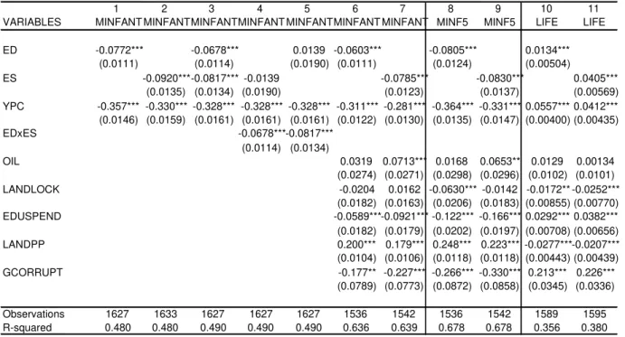
Different specifications were estimated to investigate the robustness of the evidence. Since both Infant mortality (INFANTM) and Life expectancy (LIFE) indicators tend to improve with the increase of income per capita of a country (YPC), we use YPC as a control variable in every specification and, following Owen and Wu (2007) warning that “some of the positive correlation between trade and health can be attributed to knowledge spillovers and to the fact that trade openness is associated with sound economic policies which themselves are related to better health outcomes” (Owen and Wu, 2007: 660), we also insisted in including wide range of control variables reflecting governance22 Table 6 presents the results of the estimated OLS models with robust standard errors.
22
22 Overall, our results suggest that higher levels of ED and ES are associated with lower infant mortality and higher life expectancy. Both ED and ES are linked in a significant and robust way with improving infant mortality and life expectancy. Moreover, the results were robust showing that the impact is independent of the impact of ED and ES on income per capita. These results have not been established in previous empirical literature.
Looking first to infant mortality regressions (MINFANT), the results indicate that, on average, a10% increase in the level of ED declines infant mortality by 0.77%23. Moreover, the results indicate that ED has a marginal impact of approximately one fifth of the marginal impact of per-capita income (YPC). Having a diversified export structure seems to add something extra to the economic and social setting that allows the countries to reduce more strongly the infant mortality. According to our estimates, ES has on average a stronger contributing to reduce infant mortality than ED.
Equations 4 and 5 (of Table 5) include an interaction of ED and ES variable. The result, when this variable is used simultaneously with ED or ES, suggests a process where ED is pushed by ES and reinforces the effects of ES. The combined effect of ES and ED, suggests that the contribution of sophistication reinforces that of diversification in explaining both infant mortality and life expectancy, and that the effect of each of the two variables cannot be separated24.
institutional and governance variables. For this reason the different governance variables were estimated separately. All estimated coefficients presented similar signs- The presence of these alternative governance variables did not affected significantly the signs or the significance of the coefficients of the variables ED and ES.
23This means that that if the level of export diversification of SSA increased to the average of the other
developing countries that would contribute for a reduction of 24% in the level of Infant mortality.
24
23 Testing Robustness: Including more control variables
In this section, we address the potential omitted variables bias and demonstrate that our results are robust to the inclusion of several different additional control variables. In first attempt to control for potentially omitted variables, we included additional variables in the model (See equations 6 and 7).
The estimated coefficients have the expected signal and apart from the variable LANDLOCK, they are significant at conventional levels. As shown in table, ED and ES are quite robust; the introduction of these variables seems to affect very little the size and the significance of the coefficients associated with the ED and ES variables in infant mortality regressions. Other control variables were also included, namely those reflecting the size of the economy (POP or GDP), level of education of the work force and governance (GVA, GST, GRLAW, GEFFECT, GRQ)25. The coefficients of the variables ED and ES remained significant at the 1% level. .
A similar impact of ED and ES is also found when we consider alternative dependent variables, namely the mortality rate of children under 5 years old and Life Expectancy. The results are coherent with those found for MINFANT, which appears to indicate that ED and ES have indeed an independent and robust impact on social and economic development.
Testing Robustness: Fixed Effects and Instrumental variables
In a second attempt o address potential omitted variable bias we used fixed effects technique adding dummies controls for country. The results are presented in table 7. After controlling for countries unobservable characteristics the impact of ED and ES became slight lower, but still negative and more important the coefficients are statistical significant at conventional levels. Moreover, when fixed effects are considered, the coefficients confirm that increases in ES might contribute in a more pronounced way to reduce infant mortality than proportional increases in YPC.
25 The evidence suggests that the better is the governance of each country, measured by any of the variables
24 There is another possible source of bias when Pooled OLS is used to estimate these relationships. ED and ES variables may be endogenous in the health outcome variables because social and economic development may also, at least in part, affect the decisions and process regarding ED and ES.
A common solution for the simultaneously bias is to use the Instrumental Variables (IV) estimator. Good instruments are difficult to find, since they should be simultaneously relevant and valid. That is, instrument(s) should be correlated with the endogenous regressor(s) and at the same time orthogonal to the error term.26
Another potential problem is the presence heteroskedasticity. Pagan-Hall test rejected the null hypothesis of homoskedasticity of all models tested and therefore we use the GMM method to estimate the models. Country intra-group correlation was also taken in account. We use the Stata package IVREG227 proposed by Baum et al. (2007).
The first step we undertake was to test whether the ED variable is actually endogenous in the infant mortality regression. Exogenity of both ED and ES could not be rejected in any specification28 and therefore OLS provide consistent estimates. The reliability of the C-test is nonetheless based on the quality of the (excluded) instruments; that is the relevance and validity of the instruments.. To test the relevance of the instruments we first analyze the partial R2 of the first stage regressions with the included instruments “partialled out”, which is equivalent to perform a F-test on the jointly significance of the excluded variables (instruments). F-test rejects the null hypothesis that
26
We test several alternative set of variables as potential instrumentals for ED/ES. The pre-selection of the instruments was guided by the literature. A natural choice was the lagged values of ED/ES (5 years and 10 years) We also use as instruments the Population size (and population size squared) variable. Previous work also find that population is associated with ED (e.g. Parketa and Tamberi 2008). The previous analysis suggested that “landlocked”could also be treated as an excluded instrument. There are theoretical grounds to believe that the size of the country and the fact that it is landlocked are related to ED (as previous shown) but do not directly relate with infant mortality (as well as other alternative dependent variables: INFANTM5 and LIFE). Therefore the estimated model does not include landlocked as a variable in second step. Furthermore, “landlocked” also pass the orthogonality and redundancy tests. Relevance suggested that “population squared” and 10 years lagged value were irrelevant instruments and then were not considered in the reported regressions.
27
IVREGRESS in STATA 10 would of course produce same results. The main advantage of using IVREG2 in context of only one endogeneous variable is that allows to easily test the orthogonality and relevance of the instruments
28
25 the coefficients of the instruments from the first stage regression are zero. Moreover the partial R2 are also high in every specification. Therefore the instruments pass the significance test. To validate the exclusion restrictions we employ the Hansen J statistic test. Hansen-Sargan test is an overidentification test for IV-GMM estimation routinely calculated by ivreg2. The null hypothesis is that the instruments are valid, i.e, uncorrelated with the error term. A strong rejection of the null hypothesis of the Sargan– Hansen strongly casts doubt on the validity of the estimates. Since the test fails to reject the null hypothesis it increases the confidence in our identification
Tables 8 and 9 summarize the results of the instrument variable tests.
6 – CON CLU SI ON S
In this study we investigate the political and economic factors that may contribute to successful ED and upgrading of ES strategies in the Sub-Saharan African countries. We also study the effects of ED and ES on growth and growth stability as well as in other development variables, namely infant mortality and life expectancy.
In the last decades, SSA countries exhibit very low levels of diversification, a factor that may have contributed to explain some of their income instability.
Using regression analysis in a panel of 48 SSA countries and 45 years, we confirmed that most of the findings of previous studies also apply to SSA countries, namely that the level of development and the size of the economy are positively correlated with ED. We also found that Economies with bigger populations (or GDP) also tend to have higher levels of ES.
The results about size of the economy having an important effect on both ED and ES, along with the indirect evidence, that transport costs inhibit diversification in SSA, lead us to think that economic geography factors play an important role in explaining the low levels of diversification and sophistication of the SSA exports. This suggests that increase in integration and efforts to reduce transport costs may have a positive effect in promoting ED and ES in the sub continent.
26 explain ED, 19 out of the 26 governance variables presented significant positive signs. The results were particularly robust for the World Bank variables reflecting government accountability, respect for the rule of law, political stability, effectiveness, and control of corruption.
On other way , the evidence is weak for ES. The estimated coefficients for majority of the institutional variables (15 out of 26) included in ES regressions are not statistical significant at conventional levels of significance. The evidence is not very clear about the relation of the governance and institutional factors with the sophistication of the exports in SSA. Nevertheless, the variables reflecting “transparency accountability”, and control of corruption in the public sector”, the “debt policy and fiscal policy rating”, “economic management cluster average” and the level of the “policies for social inclusion” seem to contribute in a positive way to explain the levels of ES in the SSA countries.
The results suggest that improving the education standards of the labor force is important for a successful ED strategy in SSA countries. It also suggests that increasing the lowest levels of education is likely to have a stronger effect on the ED level, while higher levels of education are more important in explaining the level of sophistication of the exports.
In the present study we also investigated the contribution of ED and ES to growth, stability and development in the SSA countries. The results, for equations in which ED and ES were used to explain GDP growth, suggest a positive relation between both ED and ES and growth. Nevertheless, this relationship was not robust.
27 In the last section we explore how ED and ES are related to socioeconomic and human development. We investigate their contribution to explain infant mortality and life expectancy, controlling for the effects of income and also for a large set of other variables.
Our results suggest that the higher the level of ED and ES the lower the infant mortality and the higher the life expectancy in SSA. The estimated coefficients are robust, although overall contribution of these variables is small. Still the estimates suggest that the impact of increasing either ED or ES in improving infant mortality is about one fifth of that of a proportional increase in GDP per capita. Moreover, the results show that the impact is independent of the impact of ED and ES on income per capita. This is an interesting and original finding that is very relevant for the SSA countries, in which GDP, exports or average income growth does not always reflect in real improvements in the life of the majority of the population.
28 GRAPHS
Graph 1. – Evolut ion of Num ber Equivalent in SSA and in t he MI D count ries
0 2 4 6 8 10 12 14 16 18
1961 1965 1969 1973 1977 1981 1985 1989 1993 1997 2001 2005
Developing excluding SSA
SSA
Graph 2 . – Evolut ion of GDP per capit a in SSA and in MI D count ries
0 500 1000 1500 2000 2500
1960 1965 1970 1975 1980 1985 1990 1995 2000 2005
Developing excluding SSA
29
Graph 3. - Evolut ion of ES ( EXPY) in SSA and in MI D count ries
0 500 1000 1500 2000 2500 3000 3500 4000 4500
1961 1966 1970 1974 1978 1982 1986 1992 1996 2000 2004
Developing excluding SSA
SSA
Graph 4. – Num ber Equivalent ( NE) and GDP per capit a in SSA
4 4.5 5 5.5 6
500 600 700 800 900 1000
GDP per-capita
30
Graph 5. – I nfant m ort alit y and num ber equivalent in SSA count ries
Graph 6. – Num ber Equivalent and life expect ancy in SSA
4 4.5 5 5.5 6
55 60 65 70
Life expectancy
Number equivalent Fitted values
60 80 100
5 10 15 20
Number equivalent
31
Graph 7. – Export sophist icat ion and life expect at ion in SSA
2000 3000 4000 5000 6000
55 60 65 70
Life expectancy
32 TABLES
TABLE 1 – Export Diversificat ion and Governance
Equation 1 2 3 4 5 6 7 8
Method RSE RSE RSE RSE RSE RSE RSE RSE
VARIABLES ED ED ED ED ED ED ED ED
POP 0.192*** 0.224*** 0.239*** 0.228*** 0.252*** 0.237*** 0.230*** 0.237*** (0.0140) (0.0106) (0.00972) (0.0101) (0.0103) (0.00978) (0.0105) (0.00982) YPC 0.233*** 0.257*** 0.186*** 0.146*** 0.160*** 0.156*** 0.155*** 0.167***
(0.0220) (0.0182) (0.0190) (0.0212) (0.0208) (0.0229) (0.0232) (0.0225) LANDLOCKED -0.429*** -0.428*** -0.409*** -0.409*** -0.422*** -0.420*** -0.426*** (0.0316) (0.0307) (0.0303) (0.0303) (0.0306) (0.0307) (0.0307) OIL -0.728*** -0.574*** -0.456*** -0.471*** -0.496*** -0.513*** -0.523*** (0.0412) (0.0410) (0.0464) (0.0487) (0.0478) (0.0473) (0.0492) LANDPC -0.0342*** -0.0339*** -0.0357*** -0.0391*** -0.0384*** -0.0381*** -0.0337***
(0.0117) (0.0108) (0.0105) (0.0106) (0.0108) (0.0109) (0.0107) EDUSPEND 0.565*** 0.570*** 0.580*** 0.549*** 0.554*** 0.561*** (0.0370) (0.0370) (0.0377) (0.0378) (0.0375) (0.0371)
GVA 0.403***
(0.0882)
GST 0.287***
(0.0737)
GCORRUPT 0.374***
(0.144)
GEFFECT 0.297**
(0.119)
GRLAW 0.200*
(0.110)
33
TABLE 2 – Det erm inant s of Export Sophist icat ion
1 2 3 4 5 6 7 8 9 10 11 12 13 14
VARIABLES ES ES ES ES ES ES ES ES ES ES ES ES ES ES
POP 0.150*** 0.145*** 0.148*** 0.152*** 0.147*** 0.151*** 0.153*** 0.162*** 0.168*** 0.167*** 0.168*** 0.181*** 0.170*** 0.171*** (0.00823) (0.00820) (0.00824) (0.00873) (0.00805) (0.00829) (0.00810) (0.0106) (0.0107) (0.0105) (0.0104) (0.0107) (0.0105) (0.0105) YPC 0.457*** 0.455*** 0.461*** 0.460*** 0.476*** 0.474*** 0.486*** 0.543*** 0.527*** 0.555*** 0.533*** 0.516*** 0.527*** 0.524*** (0.0135) (0.0140) (0.0145) (0.0138) (0.0145) (0.0155) (0.0138) (0.0297) (0.0300) (0.0295) (0.0300) (0.0294) (0.0296) (0.0296) LANDLOCK -0.0135
(0.0314)
OIL 0.0448
(0.0336)
LANDPC -0.0381*** -0.0352*** -0.0354*** -0.0363*** -0.0357*** -0.0312*** -0.0466*** -0.0441*** -0.0368*** -0.0418*** -0.0174 -0.0370** -0.0384*** (0.00977) (0.00947) (0.00942) (0.00953) (0.00950) (0.00964) (0.0139) (0.0143) (0.0142) (0.0143) (0.0143) (0.0143) (0.0144)
GVA 0.0257 (0.0680) GST 0.0467 (0.0548) GCORRUPT -0.209** (0.0877) GEFFECT -0.123 (0.0853) GRQ -0.329*** (0.0683)
GDEBT 0.166***
(0.0372)
GECON 0.0983**
(0.0471)
GPRES 0.265***
(0.0615)
GFISP 0.135***
(0.0480)
GNDR 0.530***
(0.0949)
GSOCI 0.249***
(0.0892)
GTRAN 0.176***
(0.0586)
Observations 1686 1685 1685 1685 1685 1685 1685 1402 1402 1402 1402 1402 1402 1402 R-squared 0.357 0.361 0.361 0.361 0.362 0.361 0.368 0.283 0.275 0.283 0.277 0.289 0.277 0.277
TABLE 3 - Export Diversificat ion and Educat ion
1 2 3 4 5 6 7 8 9 10 11
VARIABLES ED ED ED ED ED ED ED ES ES ES ES
POP 0.239*** 0.185*** 0.189*** 0.261*** 0.0990*** 0.100*** 0.0722* 0.153*** 0.315*** 0.259*** 0.228***
(0.00972) (0.0245) (0.0239) (0.0291) (0.0365) (0.0349) (0.0368) (0.00813) (0.0218) (0.0199) (0.0212)
YPC 0.186*** 0.360*** 0.411*** 0.455*** 0.537*** 0.560*** 0.549*** 0.482*** 0.457*** 0.332*** 0.340***
(0.0190) (0.0308) (0.0304) (0.0281) (0.0352) (0.0365) (0.0360) (0.0139) (0.0288) (0.0274) (0.0242)
LANDLOCK -0.428*** -0.245*** -0.441*** -1.025***
(0.0307) (0.0836) (0.124) (0.190)
OIL -0.574*** -1.106*** -1.049*** -0.901***
(0.0410) (0.0810) (0.0836) (0.0836)
LANDPPC -0.0339*** 0.210*** 0.160*** 0.134*** -0.0310*** -0.0221 0.00535 -0.0123
(0.0108) (0.0226) (0.0210) (0.0183) (0.00942) (0.0185) (0.0175) (0.0179)
EDUSPEND 0.565*** 0.0147
(0.0370) (0.0323)
EDUPRIM 0.331*** 0.214*** -0.0283
(0.0653) (0.0479) (0.0614)
EDUSEC 0.0319 0.0702*** 0.128***
(0.0463) (0.0266) (0.0299)
EDUTER -0.203*** 0.0863*** 0.123***
(0.0624) (0.0257) (0.0258)
Observations 1589 458 458 458 458 458 458 1595 461 461 461
34
TABLE 4 – Export diversificat ion, Growt h and St abilit y ( OLS est im at es wit h Robust standard errrors)
1 2 3 4 5 6 7 8 9 10
VARIABLES GDPG YPCG EXPORTG GDPG YPCG EXPORTG VARGDPG VARYPCG VARGDPG VARYPCG
ED 0.0541** -0.0990* 0.129*** -0.462*** -0.442***
(0.0272) (0.0547) (0.0488) (0.0403) (0.0398)
ES 0.0747** 0.229*** 0.195*** -0.318*** -0.313***
(0.0299) (0.0518) (0.0486) (0.0505) (0.0502)
Constant 1.101*** 0.641*** -2.894*** 0.618*** -1.192*** -4.176*** 3.261*** 3.193*** 5.037*** 4.960*** (0.0456) (0.0816) (0.0729) (0.220) (0.386) (0.370) (0.0604) (0.0602) (0.368) (0.365)
Observations 1590 1066 1641 1593 1069 1643 1729 1729 1734 1734
R-squared 0.002 0.004 0.005 0.004 0.018 0.009 0.054 0.050 0.022 0.022
TABLE 5 – Export diversification, Growth and Stability ( Country Fixed effects estim ates
) 1 2 3 4 5 6 7 8 9 10
GDPG YPCG EXPORTG GDPG YPCG EXPORTG VARGDPG VARYPCG VARGDPG VARYPCG
ED 0.0896** -0.0549 -0.174 -0.156** -0.128*
(0.0440) (0.0755) (0.190) (0.0673) (0.0669)
ES -0.0493 -0.00375 0.327* -0.263*** -0.258***
(0.0387) (0.0658) (0.184) (0.0583) (0.0579)
Constant 1.056*** 0.582*** -1.674*** 1.537*** 0.538 -4.414*** 2.872*** 2.794*** 4.625*** 4.551*** (0.0595) (0.105) (0.257) (0.287) (0.491) (1.418) (0.0903) (0.0897) (0.434) (0.431)
Observations 1590 1066 395 1593 1069 395 1729 1729 1734 1734
R-squared 0.003 0.001 0.002 0.001 0.000 0.009 0.003 0.002 0.012 0.012
35
TABLE 6– I nfant m ort alit y and Life expect ancy ( OLS est im at es wit h Robust st andard errors)
TABLE 7 – I nfant m ort alit y and Life expectancy ( Count ry Fixed effect s est im at es)
1 2 3 4 5 6 7 8
Fixed Effects FE FE FE FE FE FE FE FE
VARIABLES MINFANT MINFANT MINFANT MINFANT MINF5 MINF5 LIFE LIFE
ED -0.0483*** -0.0161* -0.0648*** 0.0114**
(0.0106) (0.00953) (0.0118) (0.00514)
ES -0.176*** -0.174*** -0.196*** 0.0654***
(0.00821) (0.00834) (0.00912) (0.00417)
YPC -0.141*** -0.119*** -0.113*** -0.108*** -0.156*** -0.133*** 0.0340*** 0.0188**
(0.0174) (0.0154) (0.0155) (0.0161) (0.0193) (0.0172) (0.00843) (0.00788)
EDxES -0.104***
(0.00598)
Observations 1627 1633 1627 1627 1627 1633 1680 1686
R-squared 0.058 0.261 0.262 0.199 0.064 0.263 0.014 0.140
Nº Countries 45 45 45 45 45 45 45 45
1 2 3 4 5 6 7 8 9 10 11
VARIABLES MINFANT MINFANT MINFANTMINFANT MINFANTMINFANT MINFANT MINF5 MINF5 LIFE LIFE
ED -0.0772*** -0.0678*** 0.0139 -0.0603*** -0.0805*** 0.0134***
(0.0111) (0.0114) (0.0190) (0.0111) (0.0124) (0.00504)
ES -0.0920*** -0.0817*** -0.0139 -0.0785*** -0.0830*** 0.0405***
(0.0135) (0.0134) (0.0190) (0.0123) (0.0137) (0.00569)
YPC -0.357*** -0.330*** -0.328*** -0.328*** -0.328*** -0.311*** -0.281*** -0.364*** -0.331*** 0.0557*** 0.0412***
(0.0146) (0.0159) (0.0161) (0.0161) (0.0161) (0.0122) (0.0130) (0.0135) (0.0147) (0.00400) (0.00435) EDxES -0.0678***-0.0817***
(0.0114) (0.0134)
OIL 0.0319 0.0713*** 0.0168 0.0653** 0.0129 0.00134
(0.0274) (0.0271) (0.0298) (0.0296) (0.0102) (0.0101)
LANDLOCK -0.0204 0.0162 -0.0630*** -0.0142 -0.0172** -0.0252***
(0.0182) (0.0163) (0.0206) (0.0183) (0.00855) (0.00770)
EDUSPEND -0.0589***-0.0921*** -0.122*** -0.166*** 0.0292*** 0.0382***
(0.0182) (0.0179) (0.0202) (0.0197) (0.00708) (0.00656)
LANDPP 0.200*** 0.179*** 0.248*** 0.223*** -0.0277***-0.0207***
(0.0104) (0.0106) (0.0118) (0.0118) (0.00443) (0.00439)
GCORRUPT -0.177** -0.227*** -0.266*** -0.330*** 0.213*** 0.226***
(0.0789) (0.0773) (0.0872) (0.0858) (0.0345) (0.0336)
Observations 1627 1633 1627 1627 1627 1536 1542 1536 1542 1589 1595
36
Table 8 – Pagan and Hall het eroskedast icit y t est
I NFANTM LIFE
ED ES ED ES
Pargan Statistics 114.037 140.695 43.333 44-902
37
TABLE 9 – I V ESTI MATES AND TESTS
INFANTM LIFE
ED ES ED ES
IV estimates -0.0563 (0.0303) -0.1306 (0.0646) 0.0221 (.02108) 0.0675 (0.0327) Included
Instruments
YPC LANDPP EDUSPEND OIL GCORRUPTED
Excluded instruments
Landlocked, LAGED5 , POP Landlocked, LAGES5 , POP
ENDOGENITY TESTS GMM C Statistics
0.755 4.902 0.252 2.670
Chi square P-value
0.3848 0.0268 0.6155 0.102
OVERIIDENTIFICATION RESTRICTIONS Hansen J
statistic
0.051 0.229 3.266 1.959
Chi square P-value
0.9747 0.8919 0.1954 0.3756
RELEVANCE OF INSTRUMENTS
Partial R2 0.589 0.301 0.589 0.301
38
Table A.1 Export Diversificat ion : I nst itut ional and Polit ical Variables ( OLS est im at es wit h robust st andard errors)
1 2 3 4 5 6 7 8 9 10 11 12 13
VARIABLES ED ED ED ED ED ED ED ED ED ED ED ED ED
POP 0.235*** 0.183*** 0.226*** 0.204*** 0.174*** 0.187*** 0.157*** 0.139*** 0.163*** 0.167*** 0.136*** 0.165*** 0.137*** (0.0115) (0.0126) (0.0137) (0.0124) (0.0133) (0.0138) (0.0162) (0.0172) (0.0167) (0.0169) (0.0165) (0.0169) (0.0156) YPC 0.169*** 0.160*** 0.198*** 0.144*** 0.136*** 0.202*** 0.186*** 0.189*** 0.160*** 0.149*** 0.119*** 0.140*** 0.159*** (0.0200) (0.0209) (0.0217) (0.0211) (0.0227) (0.0230) (0.0350) (0.0320) (0.0362) (0.0363) (0.0328) (0.0389) (0.0325)
EDUSPEND 0.711***
(0.0387)
GVA 1.005***
(0.0803)
GST 0.536***
(0.0611)
GCORRUPT 1.378***
(0.125)
GEFFECT 1.056***
(0.106)
GREGQUAL a) 0.411***
(0.0943)
GHRES a) 0.297***
(0.0940)
GBREG a) 0.730***
(0.105)
GDEBT a) -0.0486
(0.0420)
GECON a) -0.152***
(0.0580)
GREVN a) 0.994***
(0.0985)
GPRES a) -0.175**
(0.0696)
GFINS a) 0.988***
(0.119)
Observations 1590 1680 1680 1680 1680 1680 1398 1398 1398 1398 1398 1398 1398
R-squared 0.341 0.239 0.203 0.236 0.218 0.181 0.119 0.148 0.113 0.116 0.169 0.116 0.157
39
Table A.1 Export Diversificat ion : I nstitut ional and Polit ical Variables ( OLS
est im at es wit h robust st andard errors) ( continuat ion)
14 15 16 17 18 19 20 21 22 123 24 25 26
VARIABLES ED ED ED ED ED ED ED ED ED ED ED ED ED
POP 0.169*** 0.166*** 0.166*** 0.156*** 0.143*** 0.163*** 0.147*** 0.153*** 0.151*** 0.159*** 0.147*** 0.163*** 0.158*** (0.0167) (0.0162) (0.0170) (0.0164) (0.0169) (0.0160) (0.0161) (0.0179) (0.0160) (0.0169) (0.0162) (0.0164) (0.0164) YPC 0.131*** 0.178*** 0.157*** 0.185*** 0.152*** 0.210*** 0.190*** 0.173*** 0.200*** 0.172*** 0.186*** 0.180*** 0.179*** (0.0369) (0.0345) (0.0354) (0.0350) (0.0341) (0.0344) (0.0335) (0.0347) (0.0340) (0.0359) (0.0324) (0.0343) (0.0352) GFISP a) -0.263***
(0.0584)
GNDR a) 0.569*** (0.0992)
GMACR a) -0.125** (0.0606)
GSOCI a) 0.286***
(0.108)
GENVR 0.702*** (0.109)
GPROP a) 0.337***
(0.0801)
GPUBS a) 0.625***
(0.100)
GFINQ a) 0.141*
(0.0763)
GPADM a) 0.574***
(0.0934)
GPROT a) 0.0445
(0.109)
GSTRC a) 0.947***
(0.133)
GTRAD a) 0.359***
(0.0974)
GTRAN a) 0.172**
(0.0781)
40 Table B - Variables and Sources
VARIABLES DESCRIPTION
SOURCE
GDP GDP (constant 2000 US$) World Bank
YPC GDP per capita (constant 2000 US$) World Bank
YPCGROWTH GDP per capita growth (annual %) World Bank
POPDENS Population density (people per sq. km) World Bank
POP Population, total World Bank
EDUPRIM Labor force with at least primary education (% of total) World Bank
EDUSEC Labor force with at leastsecondary education (% of total) World Bank
EDUTERC Labor force with tertiary education (% of total) World Bank
LIFE Life expectancy at birth, total (years) World Bank
MINFANT Mortality rate, infant (per 1,000 live births) World Bank
MINF5 Mortality rate, under-5 (per 1,000) World Bank
EDUSPEND Public spending on education, total (% of GDP) World Bank
LANDPC Arable land (hectares per person) World Bank
LANDTOT Arable land (hectares) World Bank
LANDLOCKED Landlocked (dummy) UN
HERF1 Herfindahl Index (1 digit SITC rev2 ) OECD
HERF2 Herfindahl Index (2 digit) OECD
HERF3 Herfindahl Index (3 digit) OECD
HERF4 Herfindahl Index (4 digit) OECD
HERF5 Herfindahl Index (5 digit) OECD
ED Number Equivalent, based on the Herfindahl index (at 5 digit) OECD
THEIL1 Índice de Theil (1 digit, SITC Revision 2) OECD
THEIL2 Índice de Theil (2 digit, SITC Revision 2) OECD
THEIL3 Índice de Theil (3 digit, SITC Revision 2) OECD
THEIL4 Índice de Theil (4 digit, SITC Revision 2) OECD
THEIL5 Índice de Theil (5 digit, SITC Revision 2) OECD
DIST Minimum distance to EU, USA or Japan CEPII
GVA Voice and Accountability World Bank
GST Political Stability No violence World Bank
GEFFECT Government Effectiveness World Bank
GRQ Regulatory Quality World Bank
GRLAW Rule of Law World Bank
GCORRUPT Control of Corruption World Bank
EXPORTGROWTH Total Exports (Growth Rates) World Bank
EXPY1 EXPY (1 digit, SITC Revision 2) OECD
EXPY2 EXPY (2 digit, SITC Revision 2) OECD
EXPY3 EXPY (3 digit, SITC Revision 2) OECD
EXPY4 EXPY (4 digit, SITC Revision 2) OECD
EXPY EXPY (5 digit, SITC Revision 2) OECD
OIL Dummy equal to 1 for oil net exporting countries UN
SADC Dummy for the SADC countries UN
ECOWAS Dummy for the ECOWAS countries UN
SSA Dummy for the ECOWAS countries UN
41 Table B – (continuation)
VARIABLES DESCRIPTION
SOURCE
GVA Voice and Accountability World Bank
GST Political Stability No violence World Bank
GEFFECT Government Effectiveness World Bank
GRQ Regulatory Quality World Bank
GRLAW Rule of Law World Bank
GCORRUPT Control of Corruption World Bank
GHRES Building human resources World Bank
GBREG Business regulatory environment World Bank
GDEBT Debt policy rating World Bank
GECON Economic management cluster average World Bank
GREVN Efficiency of revenue mobilization World Bank
GPRES Equity of public resource use rating World Bank
GFINS Financial sector rating World Bank
GFISP Fiscal policy rating World Bank
GNDR Gender equality rating World Bank
GMACR Macroeconomic management rating World Bank
GSOCI Policies for social inclusion/equity cluster average World Bank
GENVR Policy and institutions for environmental sustainability World Bank
GPROP Property rights and rule-based governance rating World Bank
GPUBS Public sector management and institutions cluster average World Bank
GFINQ Quality of budgetary and financial management rating World Bank
GPADM Quality of public administration rating World Bank
GPROT Social protection rating World Bank
GSTRC Structural policies cluster average World Bank
GTRAD Trade rating World Bank
GTRAN Transparency, accountability, and corruption in the public sector World Bank
42
REFERENCES
Acemoglu, D. and Zilibotti, F. (1997). “Was Prometheus unbound by chance? Risk, diversification and growth”. Journal of Political Economy, 105(4): 709-751.
Ali, R., Alwang, J. and Siegel, P. (1991). "Is export diversification the best way to achieve export growth and stability? A look at three African countries". Policy Research Working Paper Series, No 729, Washington, DC.
.
Al-marhubi, F. (2000). “Export diversification and growth: an empirical investigation”. Applied economics letters, 7(9): 559–562.
Amiti, M. and Venables, A. (2002). The geography of intra-industry trade. [in:] P. J. Lloyd and H.-H. Lee (Eds.) Frontiers of Research in intra-industry trade. Palgrave Macmillan,Basingstoke.
Baum, C., Schaffer, M. and Stillman, S. (2007). “ivreg2: Stata module for extended instrumental variables/2SLS, GMM and AC/HAC, LIML and k-class regression”. Available at http://ideas.repec.org/c/boc/bocode/s425401.html.
Brenton, P. and Newfarmer, R. (2009). Watching more than the Discovery Channel to diversify exports". [in:] Richard S. Newfarmer, William Shaw and Peter Walkenhorst (Eds), Breaking into New Markets: Emerging Lessons for Export Diversification, pp. 111–124. Washington, DC: The World Bank.
Cadot, O., Carrère, C. and Strauss-Kahn, V. (2007). “Export diversification: what’s behind the hump?”. Centre for Economic Policy Research Discussion Paper, No. 6590. Costas, A., Demidova, S., Klenow, P. and Rodriguez-Clare, A. (2008). “Endogenous variety and the gains from trade”. American Economic Review Papers and Proceedings, 98(2): 444–450.
Dawe, D. (1996). “A new look at the effects of export instability on investment and growth”. World development, 24(12): 1905–1914.
De Benedictis, L., Gallegati, M. and Tamberi, M. (2009). “Overall specialisation and development:countries diversify”. The Review of World Economics (Weltwirtschaftliches Archiv), 145(1): 37–55.
Dixit, A. and Norman,V. (1980). Theory of International Trade: a dual, general equilibrium approach. Cambridge University Press, Cambridge.