Repositório Institucional UFC: O campo de Kalb Ramond com a simetria de Lorentz espontânea

(1)

UNIVERSIDADE FEDERAL DO CEARÁ CENTRO DE CIÊNCIAS

DEPARTAMENTO DE FÍSICA

PROGRAMA DE PÓS-GRADUAÇÃO EM FÍSICA

ADAILTON AZEVÊDO ARAÚJO FILHO

THE KALB RAMOND FIELD WITH SPONTANEOUS LORENTZ SYMMETRY BREAKING

(2)

ADAILTON AZEVÊDO ARAÚJO FILHO

Dissertação de Mestrado apresentada ao Pro-grama de Pós-Graduação em Física da Univer-sidade Federal do Ceará, como requisito parcial para a obtenção do Título de Mestre em Física. Área de Concentração: Física da Matéria Con-densada.

Orientador: Prof. Dr. Roberto Vinhaes Maluf Cavalcante.

(3)

Dados Internacionais de Catalogação na Publicação Universidade Federal do Ceará

Biblioteca Universitária

Gerada automaticamente pelo módulo Catalog, mediante os dados fornecidos pelo(a) autor(a)

A687t Araújo Filho, Adailton Azevedo.

The Kalb Ramond field with spontaneous Lorentz symmetry breaking / Adailton Azevedo Araújo Filho. – 2018.

68 f. : il.

Dissertação (mestrado) – Universidade Federal do Ceará, Centro de Ciências, Programa de Pós-Graduação em Física, Fortaleza, 2018.

Orientação: Prof. Dr. Roberto Vinhaes Maluf Cavalcante..

1. Lorentz violation. 2. Anti-symmetric tensor. 3. Bumblebee. 4. Weak field approximation. 5. Propagator. I. Título.

(4)

ADAILTON AZEVEDO ARAÚJO FILHO

Dissertação de Mestrado apresentada ao programa de Pós-Graduação em Física da Universidade Federal do Ceará, como requisito parcial para a obtenção do título de Mestre em Física. Área de concentração: Física da Matéria Condensada.

Aprovada em: 20/07/2018

BANCA EXAMINADORA

________________________________________ Prof. Dr. Roberto Vinhaes Maluf Cavalcante (Orientador)

Universidade Federal do Ceará (UFC)

_________________________________________ Prof. Dr. Carlos Alberto Santos de Almeida

Universidade Federal do Ceará (UFC)

_________________________________________ Dr. Manoel Messias Ferreira Júnior

(5)

(6)

ACKNOWLEDGMENTS

For starting off, I would like to thank God for His infinite kindness and mercifulness which has been given to me. Even in the moments that I felt lost, lonely and small, He was right there relaxing my soul and make me figure a way out.

Every step that I gave through my life was under their soft wings. I grew up co-cooned in their huge love heart, comforted by the clever words and motivated by their way of being. If I had a chance to live one more time, for sure, I would choose you two as being my parents again! My parents, I love you two SO MUCH. And thank you for everything.

When I was in the 5th semester, and then an undergraduate student, I knew someone who made me learn Electromagnetism I and II. After passing through some difficulties during my academic journey, I had felt quite vulnerable and confused. It turned out to be harder when I had just got my undergraduate degree and been approved to doing the master’s level. Nevertheless, that same person took me in and picked me up when I needed someone most. I always remember what he had said: Adailton, don’t be afraid! I took it on! Let’s get started! And after that, everything for me added up. He made my academic life so soft that I couldn’t have imagined. This person is someone who I’d better call him as my scientific father, Roberto Maluf.

Whenever we stumble upon difficulties around the journey of life, at least in few moments, there exist bad feelings which entirely fulfill us. We might fall down, weak, dumb... However, if you have someone who looks after you, you are able to make the guarantee that ev-erything turns out to be easier (especially when you have been doing the same course, Physics). Despite have passed some months, nowadays, I remember that place which love was released at the first time. It was 26/08/2016. In agreement with the Greek’s thoughts, which they had es-tablished the definition of happiness, which it would become to be known as a moment in which one wishes never ends. And therefore, I may guarantee for sure which the moments which we have been passing through deserve never end. Thank you for everything, Naiara Cipriano.

I would like to thank Stephen Hawking for encouraging me to do what in the cur-rents days I like most, making science. Unfortunately he passed way on the same day of my birthday.

I would like to thank Victor Santos for our fruitful discussions.

I would like to thank C.A.S.A for the disciplines taught QFT 1, QFT 2 and QFT 3 as well as for the fruitful discussions.

I would like to thank Tom Lancaster to provide me a needed inspiration for drawing difficult subjects and make them easier for understanding.

(7)

After passing through some experiences in the life, one is able to get used to either bad or good things. One of the most remarkable things which I learned is appreciating the love and

brightness which are mean content in their smile. Whenever I realized it was happening, for sure, I wish I could stop the time for the sake of the occasion never ends. Walking through the life we stumble upon a huge kind of people who turn out to belong to our daily life. However, just a few make things happen. This is my sincere homage to the people who changed

(8)

(9)

ABSTRACT

This work provides a study of some aspects of vector and tensor fields as well as their ef-fects in the context of Lorentz spontaneous symmetry breaking. Notably, we have focused on bumblebee models in which there exist a vector fieldBµwhich acquires a nonzero vacuum ex-pectation value. The study of the antisymmetric tensor, the Kalb-Ramond field, is provided as well showing a similar nonzero vacuum expectation value for the tensor fieldBµν. The

modi-fied propagator of the Kalb-Ramond field was calculated. To accomplish this, we implemented a closed algebra with six projectors which were the requirement for inverting the wave operator associated with the Lagrangian density of the theory. The massive mode, in agreement with bumblebee models, do not propagate and, therefore, do not contribute to the calculation of the interparticle potential.

(10)

LIST OF FIGURES

Figure 1 – This picture represents the closed string keep dancing on its own. It produces particles associated with its vibration. By the way, the vibrations coming from closed strings may be associated with the massless Kalb–Ramond field which has a remarkable role in my work (see Chapter 3). . . 15 Figure 2 – This Figure shows an illustration of the search for Lorentz violation as a

sig-nature of the Planck scale physics. . . 18 Figure 3 – This picture shows some interactions (dotted circles) among open and closed

strings on the worldsheet. This would lead to the so-called Lorentz sponta-neous symmetry breaking which agrees with the Bianchi identity. . . 19 Figure 4 – This picture is just an attempt of trying to visualize a preferred direction (a

vector) in spacetime after occurring the Lorentz spontaneous symmetry break-ing. . . 20 Figure 5 – The illustration of the potential V(Bµ_B

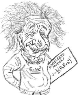
µ∓b2)(the hammer) triggering the so-called Lorentz spontaneous symmetry breaking (crashed egg) as well as the following consequences which are the appearance of Nambu-Goldstone modes (dots) and the appearance of a preferred direction (a vector) in space-time (bee with an arrow). . . 20 Figure 6 – This Figure is a comic illustration of bumblebee models. On the sheet of

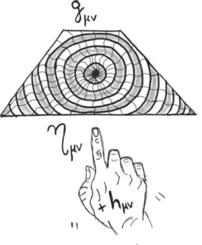
paper, is written a smooth quadratic potential which triggers Lorentz sponta-neous symmetry breaking. . . 21 Figure 7 – The metricgµν turns out to be regarded as Minkowski spacetime (ηµν) plus a

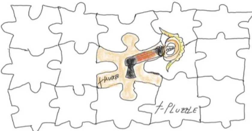
small perturbation(hµν). . . 23 Figure 8 – The t-puzzle was not undertaken up to date. Then, the phenomenological

consequences of the contribution ascribed to the fieldtµναβ _{remains an open} question. . . 38 Figure 9 – This Figure shows the bosonBµeating some Nambu Goldstone bosons which

(11)

Chapter 1 Introduction

1.1 An overview

"The standard model of particle physics describes forces and particles very well, but when you throw gravity into the equation, it all falls apart. You have to fudge the figures to make it work". - Lisa Randall [1]

Through the years, the physics has been built up by some concepts which afterwards turned out to be unified [2, 3]. In other words, it reflects some events with different phenomena which were recognized to be related to each other and some theories which were adjusted to fit in such an approach. One of the most remarkable unification happened in the early nineteenth century, the electromagnetism1_{. From 1771 through 1773, Henry Cavendish [4] tried to make}

an experiment (based on electrostatic theory) which would be known after his name, however, was Charles Augustin de Coulomb [5] who first built it up and added it up in 1785.

At the beginning of the nineteenth century, Hans Christian Oersted [6] realized that when an electric current on a wire was put nearby to the compass, its nail was deflected. Short after, André-Marie Ampère (1820–1825) [7] and Jean-Baptiste Biot Felix Savart (1820) [8] had established that the magnetic field could be produced by an alternating electric current. Following the odds of science in that epoch, a decisive step was given by Michael Faraday (1831) [9], who showed that instead of having an alternating electric current for producing a magnetic field, this field could produce an electric field as well. Equations which govern these situations were consistently added up by James Clerk Maxwell (1865) [10] which would

1_{Both physical phenomena, electricity and magnetism, were thought to be disconnected from each other.}

(13)

Introduction An overview

become to be known as Maxwell’s equations.

In the late 1960s, another fundamental unification occurred which was about one hundred years after Maxwell‘s works. This uncovered a deep relationship between the electro-magnetism and the weak interactions2_[11].

Following scientific flux, a remarkable idea was introduced by Albert Einstein [12] who made the theory of relativity3_{. In this theory, one finds out a straight conceptual unification}

of space and time [13]. In nature, the merging of space and time into a continuous media turned out to represent a new insight where all physical phenomena could take place. Newtonian mechanics [14] was rather substituted by relativistic mechanics [13], and the previous ideas of absolute time were put away. Moreover, mass and energy were shown to be correlated with each other [15]!

Another remarkable theory was brought about mainly by Erwin Schrödinger [16], Werner Heisenberg [17], and Paul Dirac [18–21]. They discovered what would be known af-terwards as Quantum Mechanics. It was verified to be a framework in which could describe correctly small bodies4_{, the microscopic world [22, 23]. In this theory, instead of having}

classi-cal variables, the new variables turn out to become operators (observables) [24–26]. Moreover, if two operators commute, their corresponding observables are able to be measured simultane-ously.

In the context of knowledge of the fundamental forces, we had better look at the gravitational one. Although was known since long ago, it was first mathematically described by Sr. Isaac Newton [14]. Afterwards, gravity was reformulated within Einstein’s theory of relativity [13]. In such an approach, the media where the events are able to take place is the so-called spacetime which borns on its own, and the gravitational force5 _{emerges due to its}

dynamical curvature [27–29]. As anyone is used to knowing, Einstein’s theory of relativity was released purely as a classical theory of gravitation rather than a quantum one. Passing through the second fundamental force, we stumble upon the electromagnetic one. In addition, it is worth remarking that Maxwell’s theory is integrally consistent with Einstein’s theory of relativity mentioned previously. Looking at the third fundamental one, which in this case, was considered as being the weak force. For instance, this is answerable for nuclear beta decay [30] in which a neutron decays into a proton6_{. Despite nuclear beta decay be known since the}

2_{For well understanding, it is highly recommended overview some key facts which happened after its}

develop-ments.

3_{It is worth mentioning that Einstein made two remarkable postulates: all inertial frame must be in agreement}

with each other and nothing could travel faster than light (causality).

4_{The fundamental particles and so forth.}

5_{In the text, this force is considered the first fundamental one.}

(14)

Introduction An overview

late nineteenth century7_{, it was not ascribed to a new force, rather it would take hold about}

the middle of the twentieth century. On the other hand, the weak interaction is much weaker than the electromagnetic one, that is why we are not able to see it working (its effects) in our daily life. For ending the discussion of these fundamental forces started above, the strong interaction [36–40] is the last one. In nowadays, it is also called the color force [41] and plays a role in holding the subatomic particles all together which are added up to forming the nuclei structure as we can see in nature. Their smallest fundamental constituents, which can not be seen in an isolated form, are called quarks [42] which are maintained coupled with each other by a tight interaction due to the color force.

It is time to come back to the subject of unification which was introduced previously. Within a consistent unified framework, in the late 1960s, the Glashow-Weinberg–Salam model of electroweak interactions [11, 43, 44] put both the electromagnetism and the weak interaction together. The theory was initially performed by regarding only massless particles whose carried the force. In nature, there exists a process called symmetry breaking [45–52] and afterwards Peter Higgs [53, 54] who gave a better interpretation which would give him the Nobel prize. Summarily, the particlesW+_, _W−_{, and the} _Z

08, which were formulated for being massless, for the sake to maintaining the gauge invariance9_{, [41, 55–58], could acquire mass due to the}

symmetry breaking process. However, in agreement with the predictions of the Standard Model, there is a remaining massless particle, the photon10_.

Due to the insufficiency of describing particles (small bodies) accurately, the clas-sical electromagnetism turned out to be substituted by the quantum electrodynamics (QED), its quantum version [35]. In this theory, the photon appears to be a quantized package [41, 55, 56, 58] (a quantum) of the electromagnetic field. In accordance with it, the theory of the weak interactions is regarded to be a quantum version as well and named quantum electroweak.

On the other hand, in the case of the strong color interaction, the quantization pro-cedure is provided as well, and the theory which governs it is considered to be quantum chro-modynamics (QCD) [59–62]. Analogously to the others forces, the carriers of the color force are eight massless particles [41, 55]. They are colored gluons [63, 64], and in accordance with quarks, they are not able to be visualized in an isolated form in nature. The quarks appear in three different colors and can be felt by gluons because they carry color.

The quantum chromodynamics together with the electroweak theory encapsulates the so-called Standard Model of particle physics [65–67]. In this model, there are interactions

7_{How strength it is given by the Fermi constant.}

8_{These three particles are the carriers of the weak interaction.}

9_{The theory which is based on the gauge symmetry reflects a "well behavior theory". In other words, the theory}

which lies in the gauge group often turns out to be renormalizable!

10_{The photon is the carrier of the electromagnetic interaction.}

(15)

Introduction String theory

between QCD and electroweak sector because some particles can feel both kinds of interactions. Until now, the Standard Model summarizes well the current knowledge of particle physics and some physicists believe that this model is only a step forward in the formulation of a complete theory [2]. As a non-perfect theory, the Standard Model has some problems such that: it does not suffice to explain the neutrino mass [68] and gravity. In addition, there is, however, a problem when one tries to incorporate the gravitational sector in the Standard Model. Due to the success of quantum theory, it is highly believed that gravity might have a quantum-like version. As a consequence of trying to make a quantum version of gravity, the resulting theory of quantum gravity has appeared to be an ill-defined [3] because it cannot be renormalized. For a better comprehension of the Big-Bang as well as certain properties of black holes, a quantum formulation of the quantum gravity seems to be reasonable. For the sake of formulating a consistent and complete theory which includes gravity, it might as well be required to build up a unified theory [3].

1.2 String theory

"String theory has the potential to show that all of the wondrous happenings in the universe - from the frantic dance of subatomic quarks to the stately waltz of orbiting binary stars; from the primordial fireball of the big bang to the majestic swirl of heavenly galaxies -are reflections of one, grand physical principle, one master equation" . - Brian Greene [69]

For a unification of all interactions present in nature, string theory is a remarkable candidate. Actually, in this theory, all kind of particles are considered to be unified since they emerge from string vibrations. In essence, string theory is a quantum theory and, since there exists gravitation within the theory, it is a quantum formulation of gravity. In this viewpoint, and bringing up the failure of Einstein’s procedure to yield a quantum version, one might make out that all others interactions are needed to get a concise description of the quantum gravitational sector.

One interesting question which we could ask ourselves would be: how the string theory can give a unified approach? The answer lies in the deep of the theory. In this theory, particles are required to be the specific vibration modes of fundamental "microscopic" strings. Analogously to the violin strings11_{, the vibrational string modes can be pointed out to}

corre-spond to the different particles which nature holds.

(16)

What about the particle decay in the context of string theory? How would be the interpretation? Whenever we stumble upon some physical decay process for instanceγ _−→ β+α(where an elementary particleγdecays intoβandα), we might as well imagine a single vibrating string which can be considered as a particleγwhich has broken into two strings which

their vibrations are associated with particlesβ andα.

The treatment of uniqueness seems to be reasonable when one considers string the-ory12_{. It would probably be demotivating to have a lot of eligible candidates for a theory of}

all forces. The indicative which string theory is unique is because it does not have adjustable dimensionless parameters13_{which are in accordance with the dimensionality of spacetime. On}

the other hand, in agreement with we have mentioned above, the Standard Model of particle physics has an average of twenty parameters which should be reorganized conveniently and then, cannot be considered unique.

As we are used to knowing, the physical spacetime is composed by one time and three-dimensional space coordinates. In the SM, this information, which is used to added up the theory, is not derived. On the other hand, within string theory, the number of dimensions emerges from the calculation and instead of four, as one is used to knowing, there exist twenty-six dimensions!

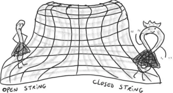
For having more details, let us start off with some subdivisions of the theory. Firstly, there exist open and closed strings. Basically, while open strings have two endpoints, closed strings have no endpoints. Secondly, there exist bosonic strings (see Figure 1) which hold in 26 dimensions, and then, bosons can be represented by their vibrations.

Figure 1: This picture represents the closed string keep dancing on its own. It produces particles associated with its vibration. By the way, the vibrations coming from closed strings may be associated with the massless Kalb–Ramond field which has a remarkable role in my work (see Chapter 3).

12_{Because all particles come from their vibrations.}

13_{String theory has one dimensionful parameter, which is called the string length}_l

s. In a roughly speaking, it

can be imagined as the "size" of string.

(17)

Another remarkable scenario, which may be most easily explained using covariant string theory, is when the Lorentz symmetry breakdown. It becomes natural when there exists an unstable perturbative string vacuum. The basic idea would be the Lorentz symmetry could be spontaneously broken by the generation of negative square masses due to the Lorentz tensor [70]. It was first investigated by Kostelecký and Samuel in 1989 [70] which had examined the covariant string field theory of open bosonic strings to figure out an attempt to explain the violation of the Poincaré group in the compactification of strings14_{. Moreover, that work}

provides the analysis whether right couplings were carried out for Lorentz symmetry breaking. Within particle field theory, spontaneous symmetry breaking can occur when the symmetry of the ground state of the theory no longer exists. This situation arises when there exists a naïve perturbed vacuum which leaves the vacuum unstable. Some fields acquire nonzero vacuum expectation values and therefore, the symmetry is spontaneously broken.

In addition, there exists another approach which borns within string theory, the Kalb-Ramond field15_{. In essence, it is a quantum field which transforms as a 2-form, an}

anti-symmetric tensor. It was firstly required when Kalb and Ramond considered the direct coupling of the area elements of the world sheets, for the sake to generalize the electromagnetic poten-tial16 _{[71]. The Kalb–Ramond field [71] could show up with the dilaton and the metric tensor}

as being massless excitations coming from closed string [3, 71, 72].

For finishing, this work is divided as follows: In Chapter 2, we make a review of the consequences due to the Lorentz violation in the gravitational scenario. It is focused on bumblebee models that the graviton couples with a vector fieldBµ. In Chapter 3, we study the

spontaneous Lorentz symmetry breaking due to an anti-symmetric 2-tensor field in Minkowski spacetime. Besides, we calculate a new complete set of spin-projection operators, which suf-ficed to evaluate the propagator of the Kalb-Ramond field in the context of Lorentz violation. In Chapter 4, we make the conclusion. In the Appendices, we explain some concepts such as: how to obtain Einstein’s equation from the variational method, the Higgs mechanism and the propagator of the Kalb-Ramond field.

14_{Because the compactification was regarded to be just an effective theory.} 15_{It was named after Michael Kalb and Pierre Ramond [71].}

16_{"The basic difference is considering in the fact that the electromagnetic potential is integrated over}

(18)

17

Chapter 2 Matter-gravity scattering

This section provides a review of the consequences due to the Lorentz violation in the gravitational scenario considering quantum gravity as an effective field theory [73]. It is focused on bumblebee models that the graviton couples with a vector field Bµ. For accom-plishing the nonrelativistic potential between two scalar particles interacting gravitationally, the calculation of the scattering matrix was performed as well.

2.1 Lorentz violation: the bumblebee models

"The other energy is the Planck scale energy, which is sixteen orders of magnitude, or ten million billion times, greater than the weak scale energy: a whopping1019 _{GeV. The} Planck scale energy determines the strength of gravitational interactions: Newton’s law says that the strength is inversely proportional to the second power of that energy. And because the strength of gravity is small, the Planck scale mass (related to the Planck scale energy by

E = mc2_{) is big. A huge Planck scale mass is equivalent to extremely feeble gravity". - Lisa} Randall [74]

(19)

Matter-gravity scattering Lorentz violation: the bumblebee models

described by the Standard Model and General Relativity. Quantum gravity effects are relevantly regarded at high energy scale in order to the Planck massmp ∼ 1.22·1019GeV, and then, up to now, as anyone could reach such scale, no evidence of any signatures of a supposed more fundamental physical phenomena have been found out. Although the Planck scale remains non-accessible experimentally, there exist some alternative ways of working on it. Some of them have been performed by exploring a different point of view which quantum gravity phenomena could be observed by highlighting its effects at attainable energies.

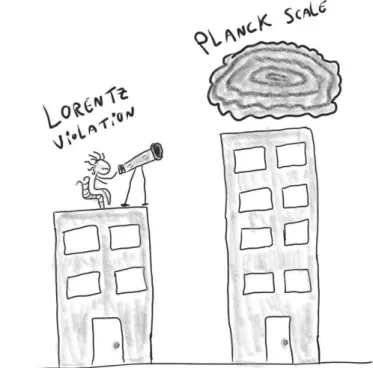
Figure 2: This Figure shows an illustration of the search for Lorentz violation as a signature of the Planck scale physics.

One of the most remarkable possibilities is Lorentz symmetry breaking [70] (see Figure 2). Lorentz violation (LV) can be seen in different contexts as, for instance, string theory [76], noncommutative field theories [77], warped brane worlds [78] and loop quantum gravity [79]. Kostelecký and Samuel proposed that due to interactions between strings could lead to spontaneous Lorentz symmetry breaking (see Figure 3).

Moreover, Kostelecký addressed the proposition of calling the Standard model plus Lorentz violation as the Standard Model Extension (SME). The SME provides a set of gauge invariant tensor operators that are in agreement with observer transformations [80] which could be used to forward Lorentz and CPT violation within the physical context.

(20)

pho-Matter-gravity scattering Lorentz violation: the bumblebee models

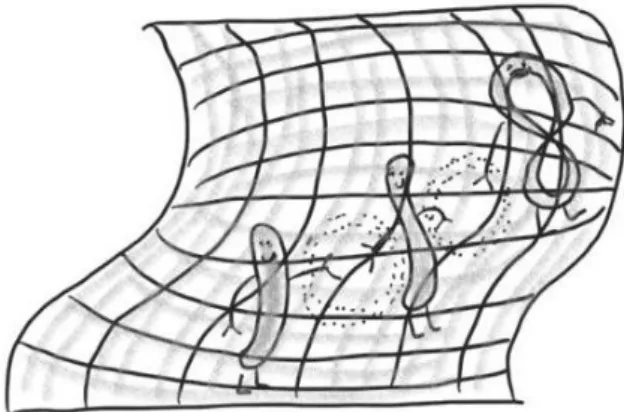
Figure 3: This picture shows some interactions (dotted circles) among open and closed strings on the worldsheet. This would lead to the so-called Lorentz spontaneous symmetry breaking which agrees with the Bianchi identity.

ton/fermion interactions [84, 85]. Some works have been pointed out Lorentz violation scenar-ios which have operators related to high dimensions giving remarkable results [86, 87]. Such high dimensional operators may also be considered within nonminimal interactions terms. On the other hand, CPT-odd nonminimal fermions coupling was first introduced in reference [88], which is trending some new developments [89, 90].

The gravitational approach has been well explored in the context of SME. It suf-fices to describe both explicit and spontaneous symmetry breaking. Nevertheless, whenever we are working on explicit symmetry breaking we stumble upon an incompatibility [91]. The continuity equation is no longer satisfied and hence, the Bianchi identity does not work. For the sake of maintaining the "previous blocks all together", we had better work on spontaneous symmetry breaking for addressing Lorentz violation in the gravitational scenario [92]. A gen-eral treatment of local Lorentz frame and diffeomorphism, within the gravitational sector of the SME, was accomplished by Bluhm and Kostelecký which says if one breaks Diffeomorphism automatically implies in breaking Lorentz symmetry and vice-versa. [93, 94]. For breaking symmetries spontaneously, is considered a vector field which acquires a nonzero vacuum ex-pectation value (VEV) [94] (see Figures 4 and 5). It represents the so-called bumblebee models (see Figure 6), which was first introduced by Kostelecký and Bluhm [94].

Moreover, there are linearized equations which may be used for studying what hap-pens to the post-Newtonian corrections [73, 95–97]. In reference [73], was investigated the low-energy effects considering Lorentz violation background in the gravitational sector of the Standard Model Extension.

(21)

Matter-gravity scattering Lorentz violation: the bumblebee models

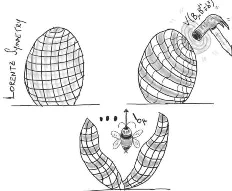
Figure 4: This picture is just an attempt of trying to visualize a preferred direction (a vector) in spacetime after occurring the Lorentz spontaneous symmetry breaking.

Figure 5: The illustration of the potentialV(Bµ_B

µ∓b2)(the hammer) triggering the so-called Lorentz spontaneous symmetry breaking (crashed egg) as well as the following consequences which are the appearance of Nambu-Goldstone modes (dots) and the appearance of a preferred direction (a vector) in spacetime (bee with an arrow).

(22)

Matter-gravity scattering The mathematical model

Figure 6: This Figure is a comic illustration of bumblebee models. On the sheet of paper, is written a smooth quadratic potential which triggers Lorentz spontaneous symmetry breaking.

term was found out in reference [73] which is proportional to_∇2 1 r ∼ δ

(3)₍_~x₎_{and may be seen} as a gravitational Darwin term [101].

2.2 The mathematical model

The simplest model regarding Lorentz-violating terms in the gravitational sector which combine fields that may break spontaneously local Lorentz frame is considered bellow as follows:

S =SEH +SLV +SM. (2.1) For starting off, let us consider the first term in equation (2.1), which is represented by the Einstein-Hilbert action1_{, given by}

SEH = Z

d4x√₋g 2

κ2(R−Λ), (2.2)

where √₋g represents the determinant of the metric gµν, R is the Ricci scalar defined as

R = gµνRµν, Λ is the so-called cosmological constant and the gravitational coupling which is represented byκ2 _{= 32}_πG_{n. It was proposed to verify the effects due to the Lorentz} viola-tion in the context of nonrelativistic potential within gravitaviola-tional sector2_.

The second term in equation (2.1) is the minimal model of the Standard Model Extension which encapsulates the coefficients (these will violate Lorentz symmetry) that are

1_{For more details how to develop Einstein’s field equation from the Einstein Hilbert action as well as the}

conservation of the Einstein’s tensor see Appendix A.

2_{We are able to neglect the consequences ascribed to}_Λ_yielding_{Λ = 0}_{from now on.}

(23)

Matter-gravity scattering Perturbation in spacetime

coupled with the RiemannRµναβ, the Ricci tensorRµν and the Ricci scalarR:

SLV = Z

d4x√₋g 2

κ2 uR+s µν

Rµν +tµναβRµναβ

, (2.3)

whereu, sµν _and_tµναβ _{are dynamical fields with zero mass dimension. It is worth mentioning} that since the sµν _and _tµναβ _{couple with the Ricci tensor}_Rµν _{and the Riemann tensor} _Rµναβ respectively, one might expect, for considering the calculations, the same symmetries of them. We consider the action (2.4) which is assumed to be a scalar (i.e. invariant under general coordinate transformations). Moreover, for the sake of obtaining the violation of the local Lorentz frame, a Higgs-like mechanism is presented3_.

Looking at the third and last term to the action (2.1) we stumble upon the matter-gravity couplings4_{. Nevertheless, it is focused on the effects due to the action (2.3), restricting}

the attention to the case whose the matter interacts exclusively with the gravitational field5_.

In agreement with the work which was made by Bailey and Kostelecký [94], let us consider a particular case wheretµναβ _{= 0}_{for simplifying the calculations. One is able to note} thatuandsµν_{have summed 10 degrees of freedom, which may be regarded as an effective field} theory with a vector fieldBµ, whose dynamics is considered when one takes down the following action:

SB = Z

d4x√₋g

−1₄BµνBµν+σBµBνRµν −V BµBµ∓b2

, (2.4)

where the field strength is given byBµν = ∂µBν −∂νBν, σ is the coupling constant (dimen-sionless), andb2_{plays the role of the vacuum expectation value due to}_B

µfield. The VEV is no longer zero and has the minimum value governed bygµνBµBν ±b2 = 0when the field gets a nonzero vacuum expectation value [70, 92, 94].

Reference [94] gives us the relation between the equation (2.3) and (2.4) which follows:

u= 1 4ξB

α_B

α, sµν =ξBµBν − 1 4ξg

µν_Bα_B

α, tµναβ = 0, (2.5) where was consideredσ = 2ξ/κ2_{for symplicity [73].}

3_{If you are interested in more details about the Higgs Mechanism see Appendix B.}

4_{They include all fields of the standard model as well as the possibility of interacting with}_u_,_sµν _and_tµναβ

which were mentioned previously.

5_{For further details involving the Lorentz-violation in the matter sector regarding the SME, one may check in}

(24)

2.3 Perturbation in spacetime

For verifying the effects due to the gravity-bumblebee coupling with the graviton propagator, one separates the dynamical fields as a vacuum solution plus fluctuations6_{. Then,}

the fieldsgµν, gµν, BµandBµcan be rewritten as follows:

gµν ₌_ηµν

−κhµν_, _g

µν =ηµν+κhµν, Bµ=bµ+ ˜Bµ, Bµ =bµ+ ˜Bµ−κbνhµν, (2.6) where_B˜_µ_and_h_µν7 _{are the previous fluctuations which we have mentioned above and}_b

µis the

Figure 7: The metricgµν turns out to be regarded as Minkowski spacetime (ηµν) plus a small perturbation(hµν).

vacuum expectation value of the bumblebee field. Before going on, let us demonstrate the last expression which appears in equation (2.6). Starting fromBµ=bµ+ ˜Bµ, one writes

gµνBν =ηµνbv+ηµνB˜ν

Bα=gµαηµνbν +ηµνB˜ν

Bα= (ηµα₋κhµα)ηµνbν+ηµνB˜ν

Bα₌_η

µνηµαbν+ηµαηµαB˜ν −κ ηµνbνhµα−κ ηµνB˜νhµα | {z } Second order

Bα=bα+ ˜Bα₋bµhµα.

(2.7)

6_{This is the standard procedure when one wants to solve an equation up to a perturbation.}

7_{Another way of seeing it is thinking of a small fluctuation around the Minkowski space (see Figure 7).}

(25)

And one might try to do the opposite. Starting withBµ _{we could get}_B

µas well. By the way, let us try to do this for the sake of verifying the veracity our previous result. It follows that

Bµ= bµ+ ˜Bµ₋bνhµν

gµσBσ =ηµσbσ +ηµσB˜σ−bνhµν

Bα =gµαηµσbσ +gµαηµσB˜σ −gµαbνhµν

= (ηµα+hµα)ηµσbσ + (ηµα+hµα)ηµσB˜σ −(ηµα+hµα)bνhµν

=ηµαηµσbσ +ηµσhµαbσ+ηµαηµσB˜σ+ηµσhµαB˜σ −ηµαhµνbν −hµαhµνbν =bα+ ˜Bα+ηµσhµαbσ−ηµαhµνbν

=bα+ ˜Bα

−→ Bµ=bµ+ ˜Bµ,

(2.8)

as we should expect.

Now, didactically let us open equation (2.4):

L ₌√₋_g_[₋1 4BµνB

µν

+σBµBνRµν−V(BµBµ∓b2)] =√₋g[₋1

4(∂µBν −∂νBµ) (∂ µ

Bν ₋∂νBµ) +σBµBνRµν−V(BµBµ∓b2)] =√₋g[₋1

4(∂µBν∂ µ

Bν ₋∂µBν∂νBµ−∂νBµ∂µBν+∂νBµ∂νBµ) +σBµBνRµν −V(BµBµ∓b2)] =√₋g[₋1

2(∂µBν∂ µ_Bν

−∂µBν∂νBµ) +σBµBνRµν −V(BµBµ∓b2)].

(2.9) Using the Euler-Lagrange for fields

δL

δBν =∂µ

δL

δ(∂µBν)

, (2.10)

and varying with respect toBµwe have attained:

δL

δBν

=√₋g[ 2σBµRµν−2V′Bν],

δL

δ(∂µBν)

=√₋g

−1₂(2∂µBν ₋2∂νBµ)

=₋√₋gBµν _{→ −}∂µ √−gBµν

,

(2.11) note that

V′ = dV dBµ

,

and plugging them all together: −√1

−g ∂

µ √ −gBµν

(26)

or,

1 √

−g ∂

µ √

−gBµν

−2V′Bν + 2σBµRµν = 0.

This equation of motion is totally in agreement with what Bailey and Kostelecký had done [94]. We choose the quadratic potential for triggering Lorentz violation:

V = λ

2 B µ_B

µ∓b2 2

. (2.13)

For calculating the modification of the graviton due to Lorentz violation, we have to previously linearize the equation of motion (2.12). For accomplishing this, we have didactically separated equation (2.12) in three parts, I,II, and III as follows:

1 √

−g ∂

µ √ −gBµν

| {z }

I

−2V′Bν | {z }

II

+ 2σBµ_R µν | {z }

III

= 0,

I : =∂µ₍_∂

µBν −∂νBµ) =∂µ∂µBν −∂µ∂νBµ=Bν −∂µ∂νBµ =

bν + ˜Bν

−∂µ∂νBµ=bν+B˜ν −∂µ∂νBµ =_b_ν ₊_B˜_ν ₋_∂_µ_∂_ν_bµ_{+ ˜}_Bµ₋_{κ b}_ν_hµν

=₋∂µ∂νB˜µ+

_b_ν ₊_B˜_ν₊_{κ ∂}_µ_∂_ν_b_ν_hµν₋_∂_µ_∂_ν_bµ

=₋∂µ∂νB˜µ+B˜ν =_η_µν_B˜µ₋_∂_µ_∂_ν_B˜µ_,

II : =₋2λhbµ_{+ ˜}_Bµ

−κbνhµν bµ+ ˜Bµ

∓b2i hbν + ˜Bν i

=₋2λhb2₊_bµ_B_˜

µ+bµB˜µ−κ bβbαhµν∓b2 i h

bν + ˜Bν i

=₋2λhb2bν +b2B˜ν+ 2bνbµB˜µ−κ bβbνbαhαβ ∓b2bν ∓b2B˜ν i

=₋4λbνbµB˜µ+ 2λκ bνbαbβhαβ,

III : = 2σbµ+ ˜Bµ₋κ bνhµν

Rµν

= 2σbµ_R

µν + ˜BµRµν −κ bνhµνRµν

= 2σbµ_R µν.

(2.14)

Adding all these terms together:

(_η_µν₋_∂_µ_∂_ν ₋₄_λb_µ_b_ν_{) ˜}_Bµ₌₋₂_{λκ b}_ν_b_α_b_β_hαβ₋₂_σbα_R_αν_, (2.15)

(27)

whereRαν =Rαν(h).

This above equation is regarded to be the linearized version of equation (2.12). After applying the Green’s function method, and putting in momentum space, one is able to check the following ansatz:

˜

Bµ= κ p µ_b

αbβhαβ 2(b_·p) +

2σbαRαµ

p2 −

2σpµ_b

αbβRαβ

p2₍_b_·_p₎ +

σpµ_R 4λ(b_·p)−

σbµ_R

p2 +

σ b2_pµ_R

p2₍_b_·_p₎ , (2.16) note that,p2 ₌_pµ_p

µ =p·p, andb·p=bµpµ.

Proof: Using the Green’s function method,

ˆ

O_µν_Gνα₍_x₋_y_{) =} _δ_µα_δ(4)₍_x₋_y₎_, (2.17)

it can be defined as a Fourier transform which follows

Gνα(x₋y) = 1 (2π)4

Z

d4p e−ip·(x−y)Gνα_(p), δ(4)(x₋y) = 1 (2π)4

Z

d4p e−ip·(x−y). (2.18) Taking into account the left terms of the linearized version of the equation of the motion repre-sented by (2.15):

(ηµν −∂µ∂ν −4λ bµbν)

| {z }

ˆ Oµν

˜

Bµ, (2.19)

follows that

(ηµν−∂µ∂ν −4λ bµbν) 1 (2π)4

Z

d4p e−ip·(x−y)Gνα_(p) =δµα 1 (2π)4

Z

d4p e−ip·(x−y), (2.20)

and,

(₋ηµνp2+pµpν−4λ bµbν) 1 (2π)4

Z

d4p e−ip·(x−y)_Gνα (p) =δµα

1 (2π)4

Z

d4p e−ip·(x−y)_. _(2.21) This entails that

Gνα(p)(−ηµνp2+pµpν−4λ bµbν) = δαµ. (2.22) Rewriting the Green’s function as a linear combination with the basis vectors,

Gνα_(p) = ã ηνα+ ˜b pνpα+ ˜c bνbα+ ˜d(pνbα+pαbν), (2.23) whereã,˜b,cãnddãre coefficients to be determined. The next step is just finding out what are

these coefficients. To accomplish this, let us work on the following expression:

(28)

Then, −˜a p2δα

µ + ˜a pµpα−4 ˜aλ bµbα

−˜b p2pµpα+ ˜b p2pµpα−4λ˜b(b·p)bµpα −˜c p2bµbα+ ˜c(b·p)pµbα−4λc b˜ 2bµbα −d p˜ 2₍_p

µbα+bµpα) + ˜d(p2pµbα+ (b·p))pµpα−d˜(4λ(b·p)bµbα+ 4λb2bµpα) =δαµ. (2.25) Considering the following basis δα

µ, pµpα, pµbα, bµpα, bµbα, we are able to solve the system of equations involving coefficients˜a,˜b,˜c,d.˜

For the basisδα

µ, we may separate the term involving only˜aas follows:

−ap˜ 2 = 1, (2.26)

and therefore,

˜

a =₋1

p2.

For the basispµpα, we may separate the terms involving˜aand˜bas follows:

˜

a₋˜b p2 + ˜b p2+ ˜d(b_·p) = 0, (2.27) and therefore,

˜

d = 1

p2₍_b_·_p₎.

For the basisbµbα, we may separate the terms involving˜a,˜candd˜as follows:

−4λ˜a₋˜c p2₋4λc b˜ 2₋4λd˜(b_·p) = 0, (2.28)

and therefore,

˜

c= 0.

For the basisbµpα, we may separate the terms involving˜bandd˜as follows:

−4λ(b_·p)₋d p˜ 2₋4λd b˜ 2 = 0, (2.29)

and therefore,

˜

b =₋(p

2_{+ 4}_{λ b}2₎ 4λ p2₍_b_·_p₎2.

(29)

Hence, the full Green’s function is given by:

Gνα (p) =−

1

p2η να

− (p

2_{+ 4}_{λ b}2₎ 4λ p2₍_b_·_p₎2 p

ν_pα₊ 1

p2₍_b_·_p₎(p

ν_bα₊_pα_bν₎_, _(2.30) or,

Gµν_(p) =₋1

p2η µν

− (p

2_{+ 4}_{λ b}2₎ 4λ p2₍_b_·_p₎2 p

µ

pν + 1

p2₍_b_·_p₎(p µ

bν+pνbµ).

Lastly, to obtain equation (2.16) is needed to couple the Green’s function with the renaming current, i.e._B˜µ ₌_Gµν

(p)(−2λκ bνbαbβh

αβ₋₂_σbα_R

αν)as follows: ˜

Bµ _{= +}2λκ ηµνbνbαbβhαβ

p2 +

2λκ bνbαbβhαβ 4λp2₍_b_·_p₎2 (4λb

2₊_p2₎_pµ_pν

− 2λκ bνbαbβh αβ

p2₍_b_·_p₎ (p

µ_bν₊_pν_bµ₎

+2ση µν_bα_R

αν

p2 +

2σbα_R αν 4λp2₍_b_·_p₎2(4λb

2₊_p2₎_pµ

pν ₋2σb

α_R αν

p2₍_b_·_p₎(p µ

bν+pνbµ)

= +_✘✘✘✘✘✘ ✘✘

2λκ bµ_b

αbβhαβ

p2 + ✘✘✘✘ ✘✘✘✘ ✘✘✘ ✘

2λκ b2_pµ₍_b

·p)bαbβhαβ

p2₍_b_·_p₎2 +

κ(b_·p)pµ_b

αbβhαβp2 2p2₍_b_·_p₎2 −_✘✘✘✘✘✘

✘✘✘

2λκ b2_pµ_b αbβhαβ

p2₍_b_·_p₎ −

✘✘✘✘

✘✘✘

✘

2λκ p2₍_b_·_p₎_bµ_b

αbβhαβ

p2₍_b_·_p₎ +2σbαR

αµ

p2 +2σb

2_bα_R ανpµpν

p2₍_b_·_p₎2 +

σbα_R

ανp2pµpν 2λp2₍_b_·_p₎2 − 2σb

α_R ανpµbν

p2₍_b_·_p₎ −

2σbα_R ανpνpµ

p2₍_b_·_p₎ ,

(2.31) where(b_·p) =bµpµ, b2 =bµbµ, p2 =pµpµ, pµbνRµν = 1₂(b·p)R. Hence we obtain,

˜

Bµ₌ κ pµbαbβhαβ 2(b_·p) +

2σbαRαµ

p2 −

2σpµ_b

αbβRαβ

p2₍_b_·_p₎ +

σpµ_R 4λ(b_·p)−

σbµ_R

p2 +

σb2_pµ_R

p2₍_b_·_p₎.

(30)

equation of motion. In this sense, (_η_µν₋_∂_µ_∂_ν ₋₄_λb_µ_b_ν_{) ˜}_Bµ_{= +}

✘✘✘✘

✘

κ ∂µ_∂µ_p

νbαbβhαβ

2(b_·p) +✘✘✘✘

✘✘✘✘

✘

2σ∂µ∂µηµνbαRαµ

p2 −_✘✘✘✘✘✘

✘✘✘

✘

2σ∂µ∂µpνbαbβRαβ

p2₍_b_·_p₎ +

✟✟

σ∂µ∂µpνR

4λ(b_·p) −✟✟

✟✟

σ∂µ∂µbνR

p2 +

✟✟

✟

σ∂µ∂µpνb2R

p2₍_b_·_p₎ −_✘✘✘✘✘✘

✘✘✘

κ ∂µ∂νpµbαbβhαβ

2(b_·p) −✘✘✘✘ ✘✘✘✘

2σ∂µ∂νbαRαµ

p2 +✘✘✘✘

✘✘✘✘

✘✘

2σ∂µ∂νpµbαbβRαβ

p2₍_b_·_p₎ −

✟✟

σ∂µ∂νpµR

4λ(b_·p) +✟✟

✟✟

σ∂µ∂νbµR

p2 −

✟✟

✟

σ∂µ∂νpµb2R

p2₍_b_·_p₎ − 4κ p

µ_b

αbβhαβλbµbν

2(b_·p) −✘✘✘✘

✘✘✘

✘

8σbαRαµλbµbν

p2 +_✘✘✘✘✘✘

✘✘✘✘

8σpµ_b

αbβRαβλbµbν

p2₍_b_·_p₎ − 4σp

µ_Rλb µbν

4λ(b_·p) +_✟✟✟

✟✟

4σbµ_Rλb µbν

p2 −✘✘✘✘

✘✘✘

✘

4σpµ_b2_Rλb µbν

p2₍_b_·_p₎ =₋2λκ bνbαbβhαβ−2σbαRνα,

(2.32) as we would like to verify.

Substituting (2.16) in (2.3), we are about to see the modification of the graviton due to the nonzero vacuum expectation value tobµ field. After noting this, let us expand the graviton-bumblebee interaction8_{. However, there are some remarks which are needed to be}

fulfilled before stepping forward. First, it is quite recommended which one has the background concerned to the linearization of the√₋g which is unusual in textbooks on general relativity.

Second, it is how to apply the previous knowledge in (2.4). As we have mentioned above, we might as well go inside to the process of linearizing√₋gwhich comes from some mathematical definitions as follows:

gµν =ηµν +hµν, log(det) = tr(log), det(η+h) = det(η)det(1 +η−1h).

8_{Remembering that we have considered only terms involving up to the second order.}

(31)

It follows, √

−g =p₋det(η+h) = elog

√

−det(η+h)

=e12log(−det(η+h)) =e[ 1

2log(−det(η)det(1+η− 1

h))]

=e[log(−detη)+12log(det(1+η− 1

h))] =p

−detηe[12log(det(1+η− 1

h))]

=p₋detηe[12tr(log((1+η− 1_h

)))] =p

−detηe h

1 2tr

η−1_h−1

2(η− 1

h)2+...i

=p₋detηe h

1 2tr(η−

1

h)₋1 4tr(η−

1

h)2+...i

=p₋detη

1 + 1

2tr η

−1_h

− 1₄tr η−1h2+ 1 2

1 2tr η

−1_h

− 1₄tr η−1h2

+O₍_h3₎

=p₋detη

1 + 1

2tr η

−1_h

− 1₄tr η−1h2+ 1 8tr

2 _η−1_h2

+O₍_h3₎

=p₋detη

1 + 1

2h µ µ− 1 4h µν

hµν+ 1 8 h

µ µ

2

+O₍_h3₎_.

(2.33) With the previous background established, we are now able to find out what would be the form of equation (2.4) after linearizing it up to the second order:

L_LV ₌_σ√₋_gBµ_Bν_R_µν ₌_σ

1 +κ1

2h α

α

BµBνRµν

=σ1 + κ 2h

α

α bµ+ ˜Bν bν + ˜Bν Rµν(h) +Rµν(h2)

=σ1 + κ 2h

α α

h

bµbνRµν(h) +bµB˜νRµν(h) +bνB˜µRµν(h) +bνbνRµν(h2) i

+O₍_h3₎

=σ1 + κ 2h

α α

h

bµbνRµν(h) + 2bµB˜νRµν(h) +bνbνRµν(h2) i

+O₍_h3₎

=σh2bµB˜νRµν(h) +bνbνRµν(h2) +

κ

2h α

αbµbνRµν(h) i

+O₍_h3₎_,

(2.34)

→ σhbνbνRµν(h2) + 2bµB˜νRµν(h) +

κ

2h α

αbµbνRµν(h) i

(32)

After passing through these calculation, let us plug (2.16) in (2.34), we obtain

L_LV ₌_ξ

p2bµbνhµνhαα+ 1 2(b·p)

2 (hα

α) 2

− 1₂(b_·p)2hµν_h

µν+p2bµbνhµαhνα

−ξ bµbνpαpβ +b(µpν)b(αpβ)hµνhαβ

+ 4ξ

κ2

−2p2bµbν −2b2pµpν + 4b·p b(µpν)−

p2_p µpν 4λ

hµνhαα

+ 4ξ 2

κ2

2bµbνpαpβ− b(µpν)b(αpβ)+

b2_p

µpνpαpβ

p2 −

2b_·p pµpν b(αpβ)

p2 +

pµpνpαpβ 4λ

hµν_hαβ

+ 4ξ 2

κ2

b2p2₋(b_·p)2+ p 4 4λ

(hα

α) 2

+ 4ξ 2

κ2

p2bµbν−2b·p b(µpν)+

(b_·p)pµpν

p2

hµνhνα+O(h3).

(2.35) It is worth mentioning that the first-order terms which appear in the gravity-bumblebee coupling constantξare quadratic order withbµ.

The Lagrangian (2.35) may be written with the expanded Einstein-Hilbert Lagrangian in the position space:

L_EH ₌_∂hµν_∂_α_hα_ν ₋_∂_µ_hµν_∂_ν_h₊1 2∂µh ∂

µ_h

− 1₂∂αhµν∂αhµν. (2.36) For the sake of convenience, we have added the convenient gauge fixing term for getting the effective Lagrangian, which is needed to obtain the modified graviton propagator as we have previously pointed out in this section:

L_GF ₌₋

∂µhµν− 1 2∂

ν_h 2

, (2.37)

whereL_GF is the Lagrangian whose accounts the gauge fixing term. In this way, the kinetic term of the graviton, as mentioned above, can be seen as

L_K ₌₋1 2h

µν_O_ˆ

µν,αβhαβ, (2.38) whereOˆ_µν,αβis an operator which may be separated in two different parts

ˆ

O_µν,αβ ₌Kˆ_µν,αβ_{+ ˆ}V_µν,αβ_, (2.39) whereVˆ_µν,αβ have terms concerned toL_LV and theKˆ_µν,αβ has a quadratic form given by:

ˆ

K_µν,αβ ₌ 1

2(ηµαηνβ +ηµβηνα−ηµνηαβ) −∂

2_. _(2.40)

Analogously with what we have been encountering in quantum field theory

(33)

books [55, 56] for the scalar field, one can write the graviton propagator as

h0_|T_{hµν(x)hαβ(y)}|0i=i Dµν,αβ(x−y), (2.41) note that theDµν,αβ(x−y)operator satisfies the so-called Green’s function equation:

ˆ

Oµν,

λσD

λσ,αβ₍_x

−y) = ˆIµν,αβ_δ(4)₍_x₋_y₎_, (2.42)

whereˆIµν,αβ_{is given by:}

ˆ

Iµν,αβ ₌ 1

2 η µα

ηνβ+ηµβηνα. (2.43)

After having seen the above considerations, for getting the graviton propagator is needed to invert the relation given by equation (2.39). The bumblebee models which we have been studying have Nambu-Goldstone (see Figure 5) and massive modes as well [96]. The following remarks involving causality and unitarity of these modes on the graviton propagator are important issues in which were well-investigated [80, 102]. Moreover, the full calculation of the graviton propagator on the presence of Lorentz violation is considered in reference [98]. Regarding the fact that the magnitude ofbµis considered small as well as the coupling constant

ξ, we have used for convenience the usual graviton propagator considered previously in equation

(2.37) and we have calculated the Lorentz-violating terms in equation (2.39) as a perturbative method presented in [103, 104]. For accomplishing the calculations, we have considered the matricial identity

1

A+B =

1

A −

1

AB

1

A+B =

1

A −

1

AB

1

A +

1

AB

1

AB

1

A+B =... (2.44)

The operatorKˆmay be inverted and then, the graviton propagator may be written regarding momentum space

Dµν,αβ₀ (q) = i 2

ηµα_ηνβ ₊_ηµβ_ηνα₋_ηµν_ηαβ

q2₊_iη . (2.45)

Now, we can show the explicit form forDµν,αβ_:

Dµν,αβ =D0µν,αβ+D µν,αβ

(34)

Matter-gravity scattering Modification of Newton’s law

Let us take a look at theDµν,αβ_LV , up to the second order:

(Dµν,αβLV )ξ =iξb2

gαβ_gµν

q2 +

qα_qβ_gµν

q4

+iξ(b·q)

2

gµν_gαβ ₋_gβµ_gαν ₋_gβν_gαµ 2q4

+iξ(b·q) b

β_bα_gµν₊_bα_bβ_gµν₊_bν_bµ_gαβ ₊_bµ_bν_gαβ 2q4

+iξ b

α_bµ_gβν ₊_bβ_bµ_gαν ₊_bα_bν_gβµ₊_bβ_bν_gαµ₋₂_bα_bβ_gµν₋₄_bµ_bν_gαβ 2q2

−4b

µ_bν_qα_qβ₊_bβ_bν_qα_qµ₊_bα_bν_qβ_qµ₊_bβ_bµ_qα_qν₊_bα_bµ_qβ_qν

2q4 ,

(2.47)

and,

(Dµν,αβLV )ξ2 = iξ2

κ2b 2

12qµ_qν₋₁₂_qα_qβ_gµν

q4 +

8qα_qβ_qµ_qν

q6

+ iξ

2_gαβ_gµν 2λκ2 −

iξ2

κ2

qα_qβ_gµν

q2λ +

iξ2

κ2

3qµ_qν_gαβ

q2_λ

+ iξ 2

κ2

2 (b_·q)2 qα_qµ_gβν ₊_qβ_qµ_gαν ₊_qα_qν_gβµ₊_qβ_qν_gαµ_{+ 2}_qµ_qν_gαβ

−2qα_qβ_gµν

q6 + iξ

2_b_·_q

κ2

10 bβ_qα_gµν₊_bα_qβ_gµν

−bν_qµ_gαβ

−bµ_qν_gαβ

q4 + iξ

2_b_·_q

κ2

8 bβ_qα_qµ_qν ₊_bα_qβ_qµ_qν

q6 − iξ

2_b_·_q

κ2

4 bµ_qα_gβν

−bµ_qβ_gαν

−bν_qα_gβµ

−bν_qβ_gαµ

q4 + iξ

2

κ2

2 bα_bµ_gβν₊_bβ_bµ_gαν ₊_bα_bν_gβµ₊_bβ_bν_gαµ

−2bα_bβ_gµν_{+ 2}_bµ_bν_gαβ

q2

+ iξ 2

κ2

28bµ_bν_qα_qβ

−bβ_bν_qα_qµ

−bα_bν_qβ_qµ

−bβ_bµ_qα_qν

−bα_bµ_qβ_qν₊ 2qα_qβ_qµ_qν

λ

q4 .

(2.48) Again it is worth mentioning that(Dµν,αβ_LV )ξ and (D_LVµν,αβ)ξ2 are contributions due

toDµν,αβ_LV which are proportional toξ and ξ2_{. Note that the product involving} _b2_, ₍_b_·_q₎2 _and (b_·q)bµ_{are first-order terms in the Lorentz violating coefficients}_u_and_sµν _{(see equation (2.3))} [73]. Therefore, one realizes that the (Dµν,αβLV )ξ enhance only first-order terms regarding u and sµν _{and, moreover, they don’t depend on the form of the bumblebee potential} _V _[73]. Considering the second order termξ, there exist expressions that are not associated with vector

bµand depending only on the coupling potential terms.

(35)

2.4 Modification of Newton’s law

In this current section we have shown the effects of Lorentz violation when one considers the modified tree-level propagator [73]. Among the variety of examples, perhaps the simplest one is the gravitational interaction of two distinguishable heavy particles which is governed by the nonrelativistic limit in the Newtonian potential. The aim is determining the scattering amplitude between two massive bosons particles mediated by the one-graviton exchange [73]. After calculating the scattering matrix amplitude, is taken the nonrelativistic limit and compared to the Born approximation for getting the modified potential taking into account the nonzero vacuum expectation value,bµ. Considering the action for a real scalar field in curved spacetime

SM = Z

d4x√₋g

1 2g

µν

∂µφ∂νφ− 1 2m

2_φ2

. (2.49)

Let us consider the following linearized relations which were expressed previously:

gµν ₌_ηµν

−κ hµν_, _(2.50)

and,

√

−g = κ 2h

µ

µ= 1 +

κ

2ηµνh µν

, (2.51)

it follows that L_M ₌_{1 +} κ

2ηµνh µν 1

2(η µν

−κhµν₎_∂

µφ∂νφ− 1 2m

2_φ2

= 1 2∂µφ∂

µ_φ − 1

2m 2_φ2

− κ 2h

µν_∂

µφ∂νφ+

κ

4h µν

ηµν∂αφ∂αφ− 1 4ηµνm

2_φ2

,

(2.52)

→ 1₂∂µφ∂µφ− 1 2m

2_φ2

− κ₂hµν∂µφ∂νφ−ηµν ∂αφ∂αφ−m2φ2

.

If one considers the scattering process governed by two scalar particles labeled after their massm1andm2, the Feynman diagram which contributes to this process is

iM_{= (}₋_iκ₎2_Vµν₍_p₁_,₋_k₁_{, m}₁₎_D_µν,αβ₍_q₎_Vαβ₍_p₂_,₋_k₂_{, m}₂₎_, (2.53)

where q = p2 − k2 = −(p1 − k1) is considered the momentum transfer and the vertex

Vµν₍_{p, k, m}₎_is

Vµν(p, k, m) = ₋1 2

pµkν +pνkµ₋ηµν p_·k+m2. (2.54)

(36)

We stumbled upon the sum of the two following terms:

iM₌_iM₀₊_iM_LV_, (2.55)

note that the first term is the usual amplitude which appears in reference [105]. It follows that

iM₀ ₌₋ iκ

2 8q2

4_{k1 ·p1 m22−k2·p2

+k1·p2k2·p1+k1 ·k2p1·p2} −2m21

− iκ 2 8q2

−2m2_1{4 m2₂₋k2·p2

+ 2k2·p2}

,

(2.56)

which it is changed due toiM_LV9. After some manipulations, one is able to see that the

non-relativistic limit is

iM_{N R} ₌iκ

2_m2 1m22 2~q2 −

iξ~b2_κ2_m2 1m22

~q2 +

iξ(~b_·~q)2_κ2_m2 1m22 2~q4 +

8iξ2_b2 0m21m22

~q2 −

iξ2_m2 1m22

2λ . (2.57)

Note that the first term gives us the tree-level result. Taking the Fourier transform, one yields the gravitational Newtonian potential [73]. Nevertheless, there are others matrix elements terms in which are concerned due to the spontaneous Lorentz violation. One is able to notice that the second and fourth terms may be absorbed by the coupling constant. The third and last terms must contribute to the matrix element and is discussed in the following text. For the sake of doing the connection with the Newtonian potential, is recommended follows the idea established in reference [106], and define the potential Fourier transformed considering the context of the nonrelativistic case

hf_|iT_|i_{i ≡}(2π)4δ(4)(p₋k)iM₍_p₁_{, p}₂ _−→_k₁_{, k}₂₎

≈ −(2π)δ(Ep−Ek)iV˜(~q),

(2.58)

and the potential may be written in the canonical position space:

V(~x) = 1 2m1

1 2m2

Z d3_q (2π)3e

i~q_·~x_V_˜₍_~q₎_. _(2.59) For solving the above equation, it considered two masses pointsm1 andm2 which lie on the coordinate vectors~x1 and~x2, where~x=~x1−~x210regarding~x, ~qand~b, one finds out the angular relations:

cosθ=~q_·~x/qr, cosθb =~b·~x/br, cos Ψ =~b·~q/bq, cos Ψ = sinθsinθbcos(φ−φb) + cosθcosθcosθb

q =_|~q_|, r =_|~x_|, b =_|~b _|.

9_{It consists of a huge expression considering the contractions of the}_b

µwith the four-momenta (of the outgoing

and incoming scalar field) and with the virtual momentum ascribed to the graviton as well.

10_{Off course, these are considered in an inertial cartesian coordinates background.}

(37)

It follows that the background vector~bis fixed in a certain direction in space of coordinates. θb andφb are also fixed angles which point out the dependence of theV(~x)[73]. Knowing all of these preliminaries, one is ready to evaluate the angular integration

Z _∞

0 dq

Z π

0

dθsinθ

Z 2π 0

dφeiqrcosθcos2Ψ = π 2_sin2_θ

b

r . (2.60)

We must calculate the momentum integral on the q-variable, ˜

V(~x) =₋GNm1m2

r

1₋3

2ξ~b 2

− 1₂ξ(~b_·xˆ)2

−GNm1m2

ξ2_b2 0 2πGN s

1

r −

ξ2 8λGN

δ3(~x)

,

(2.61) withxˆ=~x/_|~x_|. By the way, this above equation is in agreement with Refs. [94,99]. It is worth mentioning that the first-order corrections inξ, the Newtonian potential keeps showing the usual

behavior, being inversely proportional to the distance between two point masses. Moreover, this result has two remarkable features. Depending on the sign of the coupling constantξ, we can have both attractive and repulsive behavior (i.e.ξ >0is repulsive andξ <0is attractive) [73]. After some manipulations of equation (2.61) we have

V(~x) =₋GNm1m2

r

1 + 3

2s¯ 00₊1

2¯s ij

ˆ

xixˆj

+ (...). (2.62)

In accordance with reference [107], there exist a lot of discussions testing the range of gravity, which could be established experimentally the Lorentz-violating coefficients. In the following reference, is tested the accuracy of measuring how warped is the angle when a light beam deflects due to a massive body [108]. Further perspectives regarding an experimental approach are pointed out in Ref. [100] as well.

(38)

37

Chapter 3 The Kalb-Ramond field

This section provides a study of spontaneous Lorentz symmetry breaking due to an anti-symmetric 2-tensor field in Minkowski spacetime. Considering a smooth quadratic potential, the spectrum of the theory exhibits both massless and massive modes. Furthermore, we show that the massive mode is non-propagating at leading order. Besides, the massless modes in the theory can be identified with the usual Kalb-Ramond field, carrying only one on-shell degree of freedom. We provide a new complete set of spin-projection operators, which sufficed to evaluate the propagator of the Kalb-Ramond field in the context of Lorentz violation.

3.1 Lorentz violation triggered by an antisymmetric 2-tensor

Some field theories in Minkowski spacetime may be built up from p-forms, includ-ing for instance the electrodynamics (1-form), and the antisymmetric p-tensors. There exist models which have a gauge-invariant kinetic term considering the appearance of an antisym-metric 2-tensor which was first considered within string theory, the Kalb-Ramond field [71]. Another reference, which involves a straightforward approach showing remarkable properties regarding dualities to different p-form theories, was considered as well [109].