Repositório Institucional UFC: On one-loop corrections to the CPT-even Lorentz-breaking extension of QED

(1)

Vol. 33, No. 2 (2018) 1850018 (18 pages) c

World Scientific Publishing Company DOI: 10.1142/S0217751X18500185

On one-loop corrections to the

CPT-even Lorentz-breaking extension of QED

T. Mariz

Instituto de F´ısica, Universidade Federal de Alagoas, 57072-270, Macei´o, Alagoas, Brazil

tmariz@fis.ufal.br

R. V. Maluf

Departamento de F´ısica, Universidade Federal do Cear´a, Caixa Postal 6030, 60455-760, Fortaleza, CE, Brazil

r.v.maluf@fisica.ufc.br

J. R. Nascimento∗_{and A. Yu. Petrov}†

Departamento de F´ısica, Universidade Federal da Para´ıba, Caixa Postal 5008, 58051-970, Jo˜ao Pessoa, Para´ıba, Brazil

∗_{jroberto@fisica.ufpb.br} †_{petrov@fisica.ufpb.br}

Received 27 October 2017 Revised 21 December 2017 Accepted 26 December 2017

Published 19 January 2018

In this paper, we describe the quantum electrodynamics added by Lorentz-violating CPT-even terms in the context of the standard model extension. We focus our attention on the fermion sector, represented by the CPT-even symmetric Lorentz-breaking tensor

cµν. We adopt a generic form that parametrizes the components ofcµν in terms of one

four-vector, namely,cµν=uµuν−ζu 2

4 gµν. We then generate perturbatively, up to the

third order in this tensor, the aether-like term for the gauge field. Finally, we discuss the renormalization scheme for the gauge propagator, by taking into accountcµν traceless

(ζ= 1) and, trivially,cµν=uµuν(ζ= 0).

Keywords: Lorentz symmetry breaking; renormalization.

PACS numbers: 11.30.Cp, 11.15.−q

†_{Corresponding author.}

Int. J. Mod. Phys. A 2018.33. Downloaded from www.worldscientific.com

(2)

1. Introduction

The possible violation of the Lorentz symmetry is intensively discussed now. A

general framework that describes the CPT and Lorentz symmetry breaking at

low-energy level is the so-called the Standard Model Extension (SME). A typical manner

of its introduction is based on an extension of the corresponding action by new terms

involving constant vector or tensor fields which explicitly break the Lorentz

sym-metry by introducing the privileged direction of the space–time. Many examples

of such additive terms are presented in Refs. 1–4. This matter naturally calls the

interest to study of different issues related to such models, both at the classical

and at the quantum levels. Certainly, extensions of gauge field theories are of

spe-cial interest. It was shown that in the tree approximations, such theories display

highly nontrivial effects such as birefringence of waves and rotation of the plane of

polarization in the vacuum (for example, see Refs. 2, 5 and 6).

In the quantum level, these theories exhibit even more interesting properties.

The paradigmatic example is the QED with the Carroll–Field–Jackiw (CFJ) term

7

which is known to be gauge invariant, and, being generated as a quantum

correc-tion, it is finite but ambiguous (an incomplete list of references on the CFJ term

is given in Refs. 8–16). These studies certainly call the interest to consideration of

quantum properties of other Lorentz-breaking extensions of the QED. In particular,

the studies of the CPT-even Lorentz-breaking extensions of the QED are of

par-ticular importance. At the classical level, many issues related to such extensions,

especially exact solutions and dispersion relations, were studied in Refs. 17–23, and

the paper

24

_{opened an interest in these theories from the viewpoint of the extra}

dimensions concept. Further, in Refs. 25–28, the CPT-even terms were shown to

arise as quantum corrections in a CPT-odd extended QED with a nonminimal

coupling. Moreover, they turn out to be finite.

While the theory considered in Refs. 25–28 is, first, CPT-odd, second, involving

nonrenormalizable couplings (other interesting studies on quantum corrections in

nonrenormalizable Lorentz-breaking extensions of QED are presented in Refs. 29

and 30), the natural question is — whether the CPT-even contributions can be

generated from an essentially CPT-even Lorentz-breaking extension of the QED?

We note that the natural way to distinguish between CPT-even corrections arising

either from CPT-odd or from CPT-even sectors is the following. The lower possible

CPT-even correction can be already of the first order in the CPT-even

Lorentz-breaking parameter, as we will show in this paper, but it must be of the second

order in the CPT-odd Lorentz-breaking parameter, see Refs. 25 and 26, therefore, it

is natural to expect that the contribution from the CPT-even sector will dominate

since the Lorentz-breaking parameters are very small. In this paper, we use

CPT-even terms in the Maxwell and fermion sectors of SME, represented by the tensor

c

µν

, introduced in Ref. 24 and those ones in which the Lorentz-violating coefficient

is traceless, with the resulting quadratic action being essentially renormalizable in

the four-dimensional space–time.

(3)

Some preliminary results on renormalization of this model, including the

lower-order renormalization constants, were obtained already in Refs. 2 and 3. Other

important results on renormalization of Lorentz-breaking theories can be found in

Refs. 31–34, see also references therein. An alternative approach to the CPT-even

Lorentz-breaking extension of QED, involving interesting geometrical analogies, is

also presented in Ref. 35. However, it is certainly interesting to obtain the next

order aether-like counterterms. In fact, we will see that, for our two cases, the usual

renormalization constant of gauge propagator can be used to renormalize the two

contributions to the modified Maxwell actions obtained, respectively.

The structure of the paper is as follows. In Sec. 2, we introduce the

renor-malizable CPT-even extension of the QED. In Sec. 3, we calculate the one-loop

contributions to the two-point function of the gauge field, up to the third order in

c

µν

. Finally, in the summary, we discuss our results.

2. The Model

We start with the following extended QED with a CPT-even Lorentz-breaking term

(for example, see Refs. 1 and 2), given by

S

=

Z

d

4

x

¯

ψ

[

i

(

g

µν

+

c

µν

)

γ

µ

(

∂

ν

+

ieA

ν

)

−

m

]

ψ

−

1

4 F

µν

F

µν

₋

1

4 (

k

F

)

µνλρ

F

µν

_F

λρ

,

(1)

with

c

µν

=

u

µ

u

ν

−

ζ

u

2

4

g

µν

and

g

µν

= diag(1

,

−

1 ,

−

1 ,

−

1), where

c

µν

is traceless

(for

ζ

= 1) and, trivially,

c

µν

=

u

µ

u

ν

(for

ζ

= 0). We can ensure the smallness of

c

µν

requiring that

|

c

µν

| ≪

1 for any

µ, ν

. The coefficient (

k

F

)

µνλρ

, which can be

written in terms of

c

µν

, i.e. as (

k

F

)

µνλρ

=

g

µλ

c

νρ

+

g

νρ

c

µλ

−

g

µρ

c

νλ

−

g

νλ

c

µρ

, is

double traceless, (

k

F

)

µνµν

= 0, for

ζ

= 1, and (

k

F

)

µνµν

6 = 0, for

ζ

= 0. It is worth

mentioning that there are other CPT-even terms in the minimal SME, i.e. those

ones involving

d

µν

and

H

µν

(for example, see Ref. 3). These terms will not be taken

into account in this work since quantum corrections do not mix them with the

c

and

k

F

Lorentz-violating coefficients.

Our goal is to find the contributions to the purely gauge sector in the one-loop

order. So, let us write the purely spinor part of the action (1), which we will use

for quantum calculations:

S

ψ

=

Z

d

4

x

ψ i /

¯

∂

−

m

+

ic

µν

γ

µ

∂

ν

−

e /

A

−

ec

µν

γ

µ

A

ν

ψ .

(2)

The essential feature of this theory is its renormalizability in four dimensions.

Indeed, all constants in the theory are dimensionless.

Now, let us derive the Feynman rules for this theory. The kinetic term for the

spinor field is

S

kin

=

Z

d

4

x

ψ i /

¯

∂

−

m

+

ic

µν

_γ

µ

∂

ν

ψ .

(3)

(4)

=

i

p/−m

=

−

ieA/

×

=

_ic

µν

_γ

_µ

_p

_ν

_×

=

₋

_iec

µν

_γ

_µ

_A

_ν

Fig. 1. Feynman rules.

Then, the corresponding propagator is

h

ψ

(

p

) ¯

ψ

(

−

p

)

i ≡

iG

(

p

) =

i

/

p

−

m

+

c

µν

_γ

µ

p

ν

.

(4)

Within this paper, we will adopt the perturbative expansion for the free propagator:

i

/

p

−

m

+

c

µν

_γ

µ

p

ν

≃

i

/

p

−

m

+

i

/

p

−

m

(

ic

µν

_γ

µ

p

ν

)

i

/

p

−

m

.

(5)

The interaction term

S

int

=

Z

d

4

x

ψ

¯

(

−

e /

A

−

ec

µν

γ

µ

A

ν

)

ψ

(6)

gives rise to the vertices

V

1

=

−

e

ψγ

¯

µ

ψA

µ

,

(7)

V

2

=

−

e

ψγ

¯

ν

c

µν

ψA

µ

.

(8)

Graphically, these Feynman rules can be represented in Fig. 1. They will be

used to introduce one-loop Feynman diagrams.

3. Radiative Corrections and Induced Terms

The fermionic determinant in our theory can be read off from the generating

func-tional

Z

[

A

µ

] =

Z

D

ψ Dψ e

¯

iRd4

xL_ψ

=

e

iSeff

_,

₍₉₎

so that, by integrating over the fermions, we obtain the one-loop effective action

S

eff

=

−

i

Tr ln(

/

p

−

m

+

/c

· p

−

e /

A

−

e/c

· A

)

.

(10)

Here, Tr stands for the trace over the Dirac matrices, as well as the trace over

the integration in momentum and coordinate spaces, and, for brevity, we have

introduced the notation

/c

· p

=

/c

_µ

p

µ

_{, with}

_/c

µ

=

c

µν

γ

ν

.

In order to single out the quadratic terms in

A

µ

of the effective action, we

initially rewrite the expression (10) as

S

eff

=

S

eff(0)

+

∞

X

n=1

S

_eff(n)

,

(11)

(5)

where

S

_eff(0)

=

−

i

Tr ln(

/

p

−

m

+

/c

· p

) and

S

_eff(n)

=

i

n

Tr

₁

/

p

−

m

+

/c

· p

(

e /

A

+

e/c

· A

)

n

.

(12)

Then, after evaluating the trace over the coordinate space, by using the

commu-tation relation

A

µ

(

x

)

G

(

p

) =

G

(

p

−

i∂

)

A

µ

(

x

) and the completeness relation of the

momentum space, for the quadratic action

S

_eff(2)

, we get

S

_eff(2)

=

1

2 Z

d

4

x

Π

µν

_A

µ

A

ν

,

(13)

where

Π

µν

₌

_ie

2

Z

d

4

p

(2

π

)

4

tr

G

(

p

)

γ

µ

_G

₍

_p

₋

_i∂

₎

_γ

ν

_,

₍₁₄₎

with

G

(

p

) =

1 /

p

−

m

+

/c

· p

(15)

being the Feynman propagator (see Eq. (4)). Note that the derivative contained in

Π

µν

_{acts only on the first gauge field}

_A

µ

, in Eq. (13).

For the zeroth order in

c

µν

, in momentum space, we have

Π

µν0

=

ie

2

tr

Z

_d

4

_p

(2

π

)

4

S

(

p

)

γ

µ

_S

₍

_p

₋

_k

₎

_γ

ν

_,

₍₁₆₎

with

S

(

p

) = (

/

p

−

m

)

−1

_{, which yields a paradigmatic result of the usual QED}

presented in Ref. 36:

Π

µν0

=

_e

2

6 π

2

_ǫ

′

+

A

0

(

η

)

k

µ

k

ν

−

k

2

g

µν

,

(17)

where

1

ǫ′

=

1

ǫ

−

ln

m

µ′

, with

ǫ

= 4

−

D

and

µ

′2

_{= 4}

_πµ

2

_e

−γ−iπ

_{, and}

A

0

(

η

) =

e

2

36 π

2

_k

4

k

4

(6

η

tan

−1

η

+ 5)

−

12 k

2

m

2

(

η

tan

−1

η

−

1)

−

48 m

4

η

tan

−1

η

,

(18)

with

η

2

₌

k2 4m2₋

k2

. Then, for small

k

2

, we have the well-known result

Π

µν0

=

e

2

6 π

2

_ǫ

′

+

e

2

_k

2

60 π

2

_m

2

k

µ

k

ν

−

k

2

g

µν

+

· · ·

.

(19)

Then, for the effective action, we obtain the usual pole part

S

(2_eff,0)

=

−

e

2

6 π

2

_ǫ

Z

d

4

_x

1

4 F

µν

F

µν

_.

₍₂₀₎

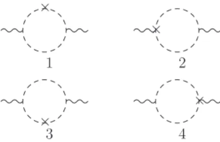
From the graphical viewpoint, the first-order Lorentz-breaking corrections are

depicted in Fig. 2.

(6)

×

1 ×

2 ×

3 ×

4

Fig. 2. First-order Lorentz-breaking contributions.

Explicitly, the contribution of the first order in

c

µν

is Π

µν1

= Π

µν

1,1

+ Π

µν

1,2

+

Π

µν1,3

+ Π

µν1,4

(see also Ref. 2), where

Π

µν1,1

=

−

ie

2

tr

Z

_d

4

_p

(2

π

)

4

S

(

p

)

/c

· pS

(

p

)

γ

µ

_S

₍

_p

₋

_k

₎

_γ

ν

_,

₍₂₁₎

Π

µν1,2

=

−

ie

2

tr

Z

_d

4

_p

(2

π

)

4

S

(

p

)

γ

µ

_S

₍

_p

₋

_k

₎

_/c

_·

₍

_p

₋

_k

₎

_S

₍

_p

₋

_k

₎

_γ

ν

_,

₍₂₂₎

Π

µν1,3

=

ie

2

tr

Z

_d

4

_p

(2

π

)

4

S

(

p

)

/c

µ

_S

₍

_p

₋

_k

₎

_γ

ν

_,

₍₂₃₎

Π

µν₁_,₄

=

ie

2

tr

Z

_d

4

_p

(2

π

)

4

S

(

p

)

γ

µ

_S

₍

_p

₋

_k

₎

_/c

ν

_.

₍₂₄₎

After the calculation of the trace and the integrals, the total result is

Π

µν₁

=

e

2

6 π

2

_ǫ

′

u

2

_k

2

₋

₂₍

_u

_·

_k

₎

2

g

µν

+ 2

u

µ

k

ν

(

u

· k

)

−

k

2

u

ν

+

k

µ

(2

u

ν

(

u

· k

)

−

u

2

k

ν

)

+

A

1

(

η

)

u

2

(

k

2

g

µν

−

k

µ

k

ν

) +

B

1

(

η

)(

u

· k

)

2

g

µν

+

C

1

(

η

)

u

µ

k

ν

(

u

· k

)

−

k

2

u

ν

+

k

µ

u

ν

(

u

· k

)

+

D

1

(

η

)(

u

· k

)

2

k

µ

k

ν

,

(25)

with

A

1

(

η

) =

e

2

_η

36 π

2

_k

4

k

4

(6 tan

−1

_η

₋

₅

_η

_{) +}

_k

2

_m

2

₍

_η

₍₉

_ζ

_{+ 8)}

₋

_{12 tan}

−1

_η

₎

−

12 m

4

(3

ζ

−

4)(

η

−

tan

−1

_η

₎

,

(26)

B

1

(

η

) =

e

2

_η

9 π

2

_k

4

k

4

(

η

−

3 tan

−1

η

)

+

k

2

m

2

(6 tan

−1

_η

₋

₇

_η

_{) + 12}

_m

4

₍

_η

₋

_tan

−1

_η

₎

,

(27)

C

1

(

η

) =

e

2

18 π

2

_k

2

_η

k

2

₍₅

_η

₋

_{6 tan}

−1

_η

_{) + 12}

_m

2

₍

_η

₋

_tan

−1

_η

₎

,

(28)

D

1

(

η

) =

e

2

_η

6 π

2

_k

6

k

2

η

(

k

2

+ 2

m

2

) + 24

m

4

(tan

−1

η

−

η

)

.

(29)

(7)

Note that the finite contributions depend on

ζ

, whereas the divergent ones do not.

We can easily observe that for small

k

2

_{, we obtain}

Π

µν₁

=

e

2

6 π

2

_ǫ

′

u

2

_k

2

₋

₂₍

_u

_·

_k

₎

2

g

µν

_{+ 2}

_u

µ

₍

_k

ν

₍

_u

_·

_k

₎

₋

_k

2

_u

ν

₎

+

k

µ

₂

_u

ν

₍

_u

_·

_k

₎

₋

_u

2

_k

ν

−

e

2

_u

2

_ζ

24 π

2

k

µ

_k

ν

₋

_k

2

_g

µν

+

e

2

120 π

2

_m

2

k

µ

4 k

2

u

ν

_u

_·

_k

₊

_k

ν

₄₍

_u

_·

_k

₎

2

₋

₍

_ζ

_{+ 2)}

_u

2

_k

2

+

k

2

(

ζ

+ 2)

u

2

k

2

−

8(

u

· k

)

2

g

µν

+ 4

u

µ

k

ν

(

u

· k

)

−

k

2

u

ν

+

· · ·

.

(30)

One can check that the pole part of this expression matches the known result.

2

It is clear that this self-energy tensor is transversal. Manifestly, the corresponding

divergent contribution to the effective action is

S

_eff(2,1)

=

e

2

6 π

2

_ǫ

Z

d

4

x

u

2

4 F

µν

F

µν

₋

_u

µ

_F

µν

u

λ

F

λν

,

(31)

which replays the structures of Maxwell term and the aether term.

24

_{It should be}

observed that if one splits the constant tensor

u

µ

u

ν

into a sum of traceless and

trace parts, i.e.

u

µ

u

ν

= ¯

c

µν

+

1₄

u

2

g

µν

(with

ζ

= 1), respectively, this divergent

contribution will be rewritten as

S

_eff(2,1)

=

−

e

2

6 π

2

_ǫ

Z

d

4

x

¯

c

µ_λ

F

µν

F

λν

,

(32)

i.e. it is completely expressed in terms of the traceless

c

µν

, namely, ¯

c

µν

.

Now, let us perform the next step which naturally consists in calculating of the

second-order aether-like quantum corrections which never considered earlier. For

the second order in

c

µν

, we have Π

µν2

= Π

µν

2,1

+ Π

µν

2,2

+ Π

µν

2,3

+ Π

µν

2,4

+ Π

µν

2,5

+ Π

µν

2,6

+

Π

µν2,7

+ Π

µν

2,8

, with

Π

µν2,1

=

ie

2

tr

Z

_d

4

_p

(2

π

)

4

S

(

p

)

/c

· pS

(

p

)

/c

· pS

(

p

)

γ

µ

_S

₍

_p

₋

_k

₎

_γ

ν

_,

₍₃₃₎

Π

µν2,2

=

ie

2

tr

Z

_d

4

_p

(2

π

)

4

S

(

p

)

/c

· pS

(

p

)

γ

µ

_S

₍

_p

₋

_k

₎

_/c

_·

₍

_p

₋

_k

₎

_S

₍

_p

₋

_k

₎

_γ

ν

_,

₍₃₄₎

Π

µν₂_,₃

=

ie

2

_tr

Z

d

4

p

(2

π

)

4

S

(

p

)

γ

µ

_S

₍

_p

₋

_k

₎

_/c

×

(

p

−

k

)

S

(

p

−

k

)

/c

· (

p

−

k

)

S

(

p

−

k

)

γ

ν

_,

₍₃₅₎

Π

µν2,4

=

−

ie

2

tr

Z

_d

4

_p

(2

π

)

4

S

(

p

)

/c

· pS

(

p

)

/c

µ

_S

₍

_p

₋

_k

₎

_γ

ν

_,

₍₃₆₎

(8)

Π

µν2,5

=

−

ie

2

tr

Z

_d

4

_p

(2

π

)

4

S

(

p

)

/c

µ

S

(

p

−

k

)

/c

· (

p

−

k

)

S

(

p

−

k

)

γ

ν

,

(37)

Π

µν₂_,₆

=

−

ie

2

tr

Z

_d

4

_p

(2

π

)

4

S

(

p

)

/c

· pS

(

p

)

γ

µ

_S

₍

_p

₋

_k

₎

_/c

ν

_,

₍₃₈₎

Π

µν2,7

=

−

ie

2

tr

Z

_d

4

_p

(2

π

)

4

S

(

p

)

γ

µ

_S

₍

_p

₋

_k

₎

_/c

_·

₍

_p

₋

_k

₎

_S

₍

_p

₋

_k

₎

_/c

ν

_,

₍₃₉₎

Π

µν2,8

=

ie

2

tr

Z

_d

4

_p

(2

π

)

4

S

(

p

)

/c

µ

S

(

p

−

k

)

/c

ν

.

(40)

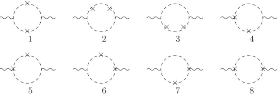
From the graphical viewpoint, the second-order Lorentz-breaking corrections are

depicted in Fig. 3. Then, the result is

Π

µν2

=

e

2

_u

2

6 π

2

_ǫ

′

(

u

· k

)

2

−

u

2

k

2

g

µν

+

u

µ

k

2

u

ν

−

k

ν

(

u

· k

)

+

k

µ

u

2

k

ν

−

u

ν

(

u

· k

)

+

A

2

(

η

)

u

2

u

µ

u

ν

+

B

2

(

η

)

u

4

k

2

g

µν

+

C

2

(

η

)

u

4

k

µ

k

ν

+

D

2

(

η

)

u

2

(

k

µ

u

ν

+

u

µ

k

ν

)(

u

· k

) +

E

2

(

η

)

u

2

(

u

· k

)

2

g

µν

+

F

2

(

η

)

u

2

(

u

· k

)

2

k

µ

k

ν

+

G

2

(

η

)(

u

· k

)

2

u

µ

u

ν

+

H

2

(

η

)(

k

µ

u

ν

+

u

µ

k

ν

)(

u

· k

)

3

+

I

2

(

η

)(

u

· k

)

4

g

µν

+

J

2

(

η

)(

u

· k

)

4

k

µ

k

ν

.

(41)

In the appendix, we present the explicit expressions for the factors

A

2

(

η

)

· · ·

J

2

(

η

),

for brevity. However, for small

k

2

_{, we can write}

Π

µν2

=

e

2

u

2

24 π

2

_ǫ

′

g

µν

u

2

k

2

(

ζ

−

4)

−

2(

ζ

−

2)(

u

· k

)

2

+ 2(

ζ

−

2)

u

µ

_k

ν

₍

_u

_·

_k

₎

₋

_k

2

_u

ν

+

k

µ

₂₍

_ζ

₋

₂₎

_u

ν

₍

_u

_·

_k

₎

₋

_u

2

₍

_ζ

₋

₄₎

_k

ν

+

e

2

_u

2

_ζ

192 π

2

g

µν

_u

2

_k

2

₍

_ζ

₋

_{6) + 12(}

_u

_·

_k

₎

2

+ 12

u

µ

k

2

u

ν

−

k

ν

(

u

· k

)

−

k

µ

12 u

ν

(

u

· k

) +

u

2

(

ζ

−

6)

k

ν

−

e

2

960 π

2

_m

2

g

µν

u

4

k

4

((

ζ

+ 4)

ζ

+ 16)

−

16 u

2

k

2

(

ζ

+ 2)(

u

· k

)

2

+ 64(

u

· k

)

4

−

8 u

µ

_k

ν

₍

_u

_·

_k

₎

₋

_k

2

_u

ν

8(

u

· k

)

2

₋

_u

2

_k

2

₍

_ζ

_{+ 2)}

+

k

µ

u

2

k

ν

8(

ζ

+ 2)(

u

· k

)

2

−

u

2

k

2

((

ζ

+ 4)

ζ

+ 16)

+ 8

u

ν

₍

_u

_·

_k

₎

_u

2

_k

2

₍

_ζ

_{+ 2)}

₋

₈₍

_u

_·

_k

₎

2

₊

_{· · ·}

_.

₍₄₂₎

It is interesting to note that, although this self-energy tensor is also transversal,

it differs from (30), since the Maxwell term and the aether term enter this

contri-bution with weights different from (30). The purely divergent contricontri-bution to the

(9)

×

1 ×

×

2 ×

×

3 ×

×

4 ×

×

5 ×

×

6 ×

×

7 ×

×

8

Fig. 3. Second-order Lorentz-breaking corrections.

effective action from this sector is

S

_eff(2,2)

=

e

2

6 π

2

_ǫ

Z

d

4

x

_u

4

16 (

ζ

−

4)

F

µν

F

µν

₋

u

2

4 (

ζ

−

2)

u

µ

_F

µν

u

λ

F

λν

.

(43)

So, we succeeded to find aether-like one-loop divergences. We note that unlike the

first-order contributions, the second-order ones essentially involve both

u

2

_{and the}

traceless ¯

c

µν

. The expression for the effective action then becomes

S

_eff(2,2)

=

e

2

6 π

2

_ǫ

Z

d

4

x

−

u

4

8 F

µν

F

µν

₊

u

2

4 ¯

c

µ

λ

F

µν

F

λν

,

(44)

where we have used again

u

µ

u

ν

= ¯

c

µν

+

1₄

u

2

g

µν

, with

ζ

= 1, in Eq. (43).

Let us finally consider the third-order Lorentz-breaking quantum correction, in

order to try to obtain a general expression for these divergent contributions. Thus,

for the third order in

c

µν

, we must calculate Π

µν3

= Π

µν

3,1

+ Π

µν

3,2

+ Π

µν

3,3

+ Π

µν

3,4

+

Π

µν3,5

+ Π

µν

3,6

+ Π

µν

3,7

+ Π

µν

3,8

+ Π

µν

3,9

+ Π

µν

3,10

+ Π

µν

3,11

+ Π

µν

3,12

, where

Π

µν3,1

=

−

ie

2

tr

Z

_d

4

_p

(2

π

)

4

S

(

p

)

/c

· pS

(

p

)

/c

· pS

(

p

)

/c

· pS

(

p

)

γ

µ

_S

₍

_p

₋

_k

₎

_γ

ν

_,

₍₄₅₎

Π

µν3,2

=

−

ie

2

tr

Z

_d

4

_p

(2

π

)

4

S

(

p

)

/c

· pS

(

p

)

/c

· pS

(

p

)

γ

µ

_S

₍

_p

₋

_k

₎

_/c

×

(

p

−

k

)

S

(

p

−

k

)

γ

ν

_,

₍₄₆₎

Π

µν3,3

=

−

ie

2

tr

Z

_d

4

_p

(2

π

)

4

S

(

p

)

/c

· pS

(

p

)

γ

µ

_S

₍

_p

₋

_k

₎

_/c

×

(

p

−

k

)

S

(

p

−

k

)

/c

· (

p

−

k

)

S

(

p

−

k

)

γ

ν

_,

₍₄₇₎

Π

µν₃_,₄

=

−

ie

2

_tr

Z

d

4

p

(2

π

)

4

S

(

p

)

γ

µ

_S

₍

_p

₋

_k

₎

_/c

_·

₍

_p

₋

_k

₎

_S

₍

_p

₋

_k

₎

_/c

×

(

p

−

k

)

S

(

p

−

k

)

/c

· (

p

−

k

)

S

(

p

−

k

)

γ

ν

_,

₍₄₈₎

Π

µν3,5

=

ie

2

tr

Z

_d

4

_p

(2

π

)

4

S

(

p

)

/c

· pS

(

p

)

/c

· pS

(

p

)

/c

µ

_S

₍

_p

₋

_k

₎

_γ

ν

_,

₍₄₉₎

(10)

Π

µν3,6

=

ie

2

tr

Z

_d

4

_p

(2

π

)

4

S

(

p

)

/c

· pS

(

p

)

/c

µ

S

(

p

−

k

)

/c

· (

p

−

k

)

S

(

p

−

k

)

γ

ν

,

(50)

Π

µν₃_,₇

=

ie

2

tr

Z

_d

4

_p

(2

π

)

4

S

(

p

)

/c

µ

_S

₍

_p

₋

_k

₎

/c

×

(

p

−

k

)

S

(

p

−

k

)

/c

· (

p

−

k

)

S

(

p

−

k

)

γ

ν

_,

₍₅₁₎

Π

µν3,8

=

ie

2

tr

Z

_d

4

_p

(2

π

)

4

S

(

p

)

/c

· pS

(

p

)

/c

· pS

(

p

)

γ

µ

_S

₍

_p

₋

_k

₎

_/c

ν

_,

₍₅₂₎

Π

µν3,9

=

ie

2

tr

Z

_d

4

_p

(2

π

)

4

S

(

p

)

/c

· pS

(

p

)

γ

µ

_S

₍

_p

₋

_k

₎

_/c

_·

₍

_p

₋

_k

₎

_S

₍

_p

₋

_k

₎

_/c

ν

,

(53)

Π

µν₃_,₁₀

=

ie

2

_tr

Z

d

4

p

(2

π

)

4

S

(

p

)

γ

µ

_S

₍

_p

₋

_k

₎

_/c

×

(

p

−

k

)

S

(

p

−

k

)

/c

· (

p

−

k

)

S

(

p

−

k

)

/c

ν

,

(54)

Π

µν₃_,₁₁

=

−

ie

2

tr

Z

_d

4

_p

(2

π

)

4

S

(

p

)

/c

· pS

(

p

)

/c

µ

_S

₍

_p

₋

_k

₎

/c

ν

,

(55)

Π

µν3,12

=

−

ie

2

tr

Z

_d

4

_p

(2

π

)

4

S

(

p

)

/c

µ

_S

₍

_p

₋

_k

₎

_/c

_·

₍

_p

₋

_k

₎

_S

₍

_p

₋

_k

₎

_/c

ν

_.

₍₅₆₎

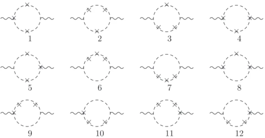
These third-order corrections are depicted in Fig. 4. Then, the total result can

be written as

Π

µν3

=

e

2

_u

4

96 π

2

_ǫ

′

g

µν

_u

2

_k

2

₍

_ζ

₋

₄₎

2

₋

₂₍₍

_ζ

₋

₄₎

_ζ

_{+ 8)(}

_u

_·

_k

₎

2

+ 2((

ζ

−

4)

ζ

+ 8)

u

µ

_k

ν

₍

_u

_·

_k

₎

₋

_k

2

_u

ν

+

k

µ

2((

ζ

−

4)

ζ

+ 8)

u

ν

(

u

· k

)

−

u

2

(

ζ

−

4)

2

k

ν

+ finite terms

,

(57)

where we have calculated only the divergent terms. We have omitted the finite

terms because up to now we are interested in interring a general expression for the

renormalization constant of the gauge propagator. Thus, by taking into account

(13), the effective action becomes

S

_eff(2,3)

=

e

2

6 π

2

_ǫ

Z

d

4

x

u

6

64 (

ζ

−

4)

2

_F

µν

F

µν

−

u

4

16 ((

ζ

−

4)

ζ

+ 8)

u

µ

_F

µν

u

λ

F

λν

.

(58)

Rewriting the above expression in terms of traceless ¯

c

µν

, we obtain

S

(2_eff,3)

=

e

2

6 π

2

_ǫ

Z

d

4

x

u

6

16 F

µν

F

µν

₋

5

16 u

4

_c

_¯

µ

λ

F

µν

F

λν

.

(59)

(11)

×

1 ×

×

2 ×

×

3 ×

×

4 ×

×

5 ×

×

6 ×

_×

×

7 ×

×

8 ×

×

9 ×

×

10 ×

×

11 ×

×

12

Fig. 4. Third-order Lorentz-breaking corrections.

Finally, the complete one-loop divergent contribution to the two-point function,

for

ζ

= 0, is given by the sum of (20), (31), (43), (58). Thus, we have

S

_eff(2)

=

−

e

2

6 π

2

_ǫ

Z

d

4

x

₁

4 (1

−

u

2

₊

_u

4

₋

_u

6

₎

_F

µν

F

µν

+

1 −

u

2

2 +

u

4

2 u

µ

_F

µν

u

λ

F

λν

+

· · ·

.

(60)

By analyzing the above expression, we can easily write the general pole part result as

S

_eff(2)

=

−

e

2

6 π

2

_ǫ

Z

d

4

x

1

4 (1 +

u

2

₎

−1

_F

_˜

µν

F

˜

µν

,

(61)

where

˜

F

µν

= (

g

µα

+

u

µ

u

α

)(

g

νβ

+

u

ν

u

β

)

F

αβ

,

(62)

which is, in fact, the expression we should have when considering the

nonperturba-tive propagator (4). Formally, here we have an effecnonperturba-tive metric ˜

g

µα

=

g

µα

+

u

µ

u

α

,

and

S

_eff(2)

is proportional to ˜

g

µν

˜

g

αβ

F

µα

F

νβ

, which replays the form of the Lagrangian

of the electromagnetic field in a curved space. Thus, we must modify the

Lorentz-violating Maxwell action in (1), as follows:

S

A

=

−

1

4 Z

d

4

_x

_{(1 +}

_u

2

₎

−1

_F

_˜

µν

F

˜

µν

,

(63)

so that the renormalization constant is given by the usual one

Z

3

= 1

−

e

2

6 π

2

_ǫ

,

(64)

in which the coefficient (1 +

u

2

₎

−1

_{can be absorbed in the renormalization}

con-stant of the generating functional. Note that we can rewrite the modified Maxwell

(12)

Lagrangian as

LA

=

−

1

4 F

˜

µν

F

˜

µν

₌

₋

1

4 F

µν

F

µν

₋

1

4 (

k

F

)

µνλρ

F

µν

_F

λρ

_,

₍₆₅₎

where

(

k

F

)

µνλρ

=

1 +

u

2

2 (

g

µλ

u

ν

u

ρ

+

g

νρ

u

µ

u

λ

−

g

µρ

u

ν

u

λ

−

g

νλ

u

µ

u

ρ

)

.

(66)

This expression for (

k

F

)

µνλρ

was used in Ref. 37, in order to keep the Lagrangian

formally covariant, as we are observing, however, here, it is the first time that it

has been obtained through radiative corrections.

Now, let us discuss the more interesting case, when

c

µν

is traceless, by

con-sidering the sum of (20), (32), (44), (59). The effective action of the pole part is

given by

S

_eff(2)

=

−

e

2

6 π

2

_ǫ

Z

d

4

x

1

4 1 +

u

4

2 −

u

6

4 F

µν

F

µν

+

1 −

u

2

4 +

5 u

4

16 ¯

c

µ_λ

F

µν

F

λν

+

· · ·

.

(67)

Then, by analyzing the above equation, the general result is trivially written as

S

_eff(2)

=

−

e

2

6 π

2

_ǫ

Z

d

4

x

1

4 1 +

3 u

2

4

−1

1 −

u

2

4

−3

¯

F

µν

F

¯

µν

,

(68)

with now

¯

F

µν

= (

g

µα

+ ¯

c

µα

)(

g

νβ

+ ¯

c

νβ

)

F

αβ

,

(69)

so, one has the effective metric ¯

g

µα

=

g

µα

+ ¯

c

µα

which again allows to write the

S

eff(2)

as a result proportional to ¯

g

µν

¯

g

αβ

F

µα

F

νβ

. Therefore, for this case, the modified

Maxwell action must assume the form

S

A

=

−

1

4 Z

d

4

_x

1 +

3 u

2

4

−1

1 −

u

2

4

−3

¯

F

µν

F

¯

µν

,

(70)

where again the renormalization constant is the usual one (64). By rewriting the

above action in terms of traceless ¯

c

µν

, we also obtain the Lagrangian

LA

=

−

1

4 F

¯

µν

F

¯

µν

₌

₋

1

4 F

µν

F

µν

₋

1

4 (

k

F

)

µνλρ

F

µν

_F

λρ

_,

₍₇₁₎

with

(

k

F

)

µνλρ

= 4

g

µλ

¯

c

νρ

+ 4¯

c

µλ

c

¯

νρ

+ 2

g

µλ

c

¯

να

¯

c

αρ

+ 4¯

c

µλ

¯

c

να

¯

c

αρ

+ ¯

c

µα

c

¯

αλ

¯

c

νβ

¯

c

βρ

,

(72)

which is more involved than (66), but can be reduced to it by replacing, formally,

¯

c

µν

by

u

µ

u

ν

, i.e. we get (

k

F

)

µνλρ

= (4 + 2

u

2

)

g

µλ

u

ν

u

ρ

.

(13)

Let us now discuss the general structure of quantum corrections of different

orders in insertions. The examples presented above showed that the generic result

with

n

insertions will look like

S

_eff(2)_{, n}

=

−

e

2

π

2

_ǫ

Z

d

4

x a

n

u

2n

F

µν

F

µν

+

b

n

u

2n −2

_¯

_c

µ

λ

F

µν

F

λν

,

(73)

where the coefficients

a

n

,

b

n

are some numbers. It is the only possible form for

such corrections. However, one cannot determinate a precise form of the

a

n

,

b

n

without explicit calculations, and there is no any

a priori

reason for existence of

any relations between these coefficients.

4. Summary

In this paper, for the CPT-even Lorentz-breaking extension of QED, we showed

that the aether term naturally arises as a quantum correction, and succeeded to

calculate the unique renormalized modified Maxwell action to the third order in a

constant symmetric second-rank tensor

c

µν

, for which, in its part, we considered all

possible structures, from the traceless one up to the direct product of two constant

vectors. In the four-dimensional case, it diverges which requires an introduction

of corresponding counterterms, both in Maxwell and in aether sectors. Actually,

it involves only one renormalization constant (64), so that, in principle, one needs

to modify the Maxwell action already at the tree level (see Eqs. (63) and (70)).

By rewriting these actions in terms of (

k

F

)

µνλρ

, we obtained the expressions (66)

and (72), respectively, which are the all-insertion contributions for the CPT-even

Lorentz-breaking extension of Maxwell theory. It is interesting to note that for the

light-like

u

µ

, only the lower order in

u

µ

yields nontrivial contributions both to the

Maxwell and to the aether terms. We note that, unlike,

35

_{in the four-dimensional}

space–time we succeeded to calculate not only the divergent part but also the finite

one of the CPT-even term. Also, the results which should be mentioned here are,

first, the fact that within our calculations, we for the first time obtained explicitly

through radiative corrections the covariantized Lagrangian (66) which earlier

37

_was

shown to arise within a completely distinct context, that is, the calculation of the

free energy; second, we generalized this coefficient for the essentially traceless

c

µν

;

third, we demonstrated that the result, involving both Maxwell and aether terms,

is characterized by only one renormalization constant.

The importance of our results consists in the fact that in the four-dimensional

space–time our theory is renormalizable in all orders in all

c

µν

insertions, just

as the electrodynamics with the CFJ term.

7

_{Another important feature of our}

theory consists in arising of an effective metric looking like ˜

g

µν

=

g

µν

+

u

µ

u

ν

or ¯

g

µν

=

g

µν

+ ¯

c

µν

. In principle, the calculations in resulting theory obtained

through summation of the tree-level Maxwell term and the quantum correction

can be carried out with the use of this effective metric implying in appropriate

modification of vertices and propagators formulated in the new space with the

metric ˜

g

µν

or ¯

g

µν

. We note that in Ref. 34, where the effective metric arises due to

(14)

the Lorentz-breaking modification of the Dirac matrices, the results were obtained,

first, only in the spinor sector, second, only up to the first order in Lorentz-breaking

parameters, and in Ref. 35 the effective metric has been introduced already on the

step of consideration of the classical action, while we show how it arises as a result

of summation of quantum corrections of different orders in ¯

c

µν

or

u

µ

u

ν

. Therefore,

the space–time turns out to be the affine one (see also discussions in Refs. 34 and

35), as it occurs for the CPT-even supersymmetric Lorentz-breaking theories.

38,39

It is natural to expect that it can open the way to implement the Lorentz symmetry

breaking within the supergravity. The possible way to do it is as follows: we consider

the Lorentz-breaking supersymmetry algebra discussed in Ref. 38, and suggest the

Lorentz-breaking tensor

c

µν

(which in Ref. 38, it has been chosen in the simplest

form

c

µν

=

u

µ

u

ν

) to be a fixed function of space–time coordinates rather than

constant. This clearly would imply in a more sophisticated algebra of supercovariant

derivatives, and in this case the effective metric clearly will not be more an affine

one, implying in a nonzero curvature, hence we face a problem of studying the

supersymmetric theory on a curved background, that is, coupled to a supergravity.

We expect to study this problem in one of our next papers.

Acknowledgments

This work was partially supported by Conselho Nacional de Desenvolvimento

Cient´ıfico e Tecnol´ogico (CNPq). The work by A. Yu. Petrov has been supported