Stock returns, inflation, and real activity in developing countries: A Markov-switching approach

PANOECONOMICUS, 2015, Vol. 62, Issue 1, pp. 55-76

Received: 24 December 2012; Accepted: 22 May 2014.

UDC 336.763.2:330.43 DOI: 10.2298/PAN1501055C Original scientific paper

Atilla Cifter

School of Economics and Administrative Sciences, Istanbul Kemerburgaz University, Turkey

atilla.cifter@kemerburgaz.edu.tr

Stock Returns, Inflation, and Real

Activity in Developing Countries:

A Markov-Switching Approach

Summary: This paper empirically investigates the relationship between real stock returns, inflation, and real activity using the Markov-switching dynamic regression (MS-DR) approach. The MS-DR allows multiple structural breaks in the estimation, and we can check regression coefficients separately in the recession and expansion periods. We selected two major developing countries (Mexico and South Africa) in order to reduce location bias. We use real stock returns, expected inflation, unexpected inflation, and real GDP growth in the estimations, and the ARFIMA model is used for unexpected inflation. The em-pirical results show that the relationship between real stock returns and inflation is negative only in the recession period. This regime-dependency is also tested with Eugene F. Fama’s (1981) proxy effect hypothesis, and it is found that the stock returns respond differently to inflation in a regime according to the re-gime-dependent proxy effect hypothesis. These findings suggest that the nega-tive relationship puzzle in the empirical finance literature can be explained with the regime-dependency effect.

Key words: Fisher hypothesis, Regime-dependent proxy effect hypothesis, Real stock returns, Inflation, MS-DR approach.

JEL: E31, G10, C32.

The Fisher hypothesis (Irving Fisher 1930) states that nominal interest should fully reflect changes in inflation. This relationship can also be generalised to the asset market. If the Fisher hypothesis holds, common stocks can be a hedge for inflation, and this hypothesis is called as “generalized Fisher effect”. In recent studies, Mo-hammad S. Hasan (2008), Paul Alagidede and Theodore Panagiotidis (2012), Hsiao-Fen Chang (2013) find evidence that stock returns hedge against inflation. In contrast to the Fisher hypothesis, many empirical studies have shown either a negative or no significant correlation between stock returns and inflation (see, e.g. Fama and G. William Schwert 1977; Keun Yeong Lee 2008; Kryzanowski Lawrence and Abdul H. Rahman 2009; Stella Karagianni and Catherine Kyrtsou 2011; Yu Hsing and Wen-jen Hsieh 2012; Jeffrey Oxman 2012).

nega-56 Atilla Cifter

tive only in the recession period. This regime-dependent negative relationship is also tested with Fama’s (1981) proxy effect hypothesis, and it is found that the stock re-turns respond differently to inflation in a regime, according to the regime-dependent proxy effect. These findings suggest that the negative relationship puzzle in the em-pirical literature can be explained with the regime-dependency between real stock returns, inflation, and real activity.

The remainder of this paper is organised as follows. The next section reviews previous literature on the Fisher and the proxy effect hypotheses. The methodology of the MS-DR approach is presented in the second section. In the third section, the data is presented and empirical results are discussed. The summary is presented in the final section.

1. Literature Review

After the inflationary period in the 1970s, Fama and Schwert (1977) examine the Fisher hypothesis for stock returns. They find that common stocks are a poor hedge against expected and unexpected inflation in the U.S. According to the authors, there might also be a negative correlation between stock returns and inflation. Same as this study, Zisimos Koustas and Apostolos Serletis (1999) reject the Fisher hypothesis in the long-run for OECD countries. Jakob B. Madsen, Ratbek Dzhumashev, and Hui Yao (2013) test the Fisher hypothesis for 20 OECD countries over the period 1870-2006, and they find that the relationship between stock returns and growth is only positive when output volatility is persistent. Using autoregressive distributive lag bounds approach, Mustabshira Rushdi, Jae H. Kim, and Param Silvapulle (2012) find that there is a significant negative relationship between observed inflation and real stock returns for Australia.

The relationship between stock returns and inflation for developing countries is as puzzling as the findings in developed countries. N. Bulent Gultekin (1983) firstly tests the Fisher hypothesis for both of the developed and developing countries. He finds that the stock return-inflation relation is not stable over time and that there are significant differences among countries. On the other hand, he finds Israel and the UK have statistically positive coefficient. Claude B. Erb, Campbell R. Harvey, and Tadas E. Viskanta (1995) test the interaction between inflation and expected stock returns in 21 developed and 20 developing countries. Their results confirm the negative relationship between realised inflation and realised asset returns for all of the countries in the sample. Jaeuk Khil and Bong-Soo Lee (2000) examine the rela-tionship between real stock returns and inflation in the U.S. and ten Pacific-rim coun-tries. They find that nine developing countries reflect a negative relationship between real stock returns and inflation; however, Malaysia is the only country that exhibits a positive relation. Alagidede (2009) examines the Fisher hypothesis for six African countries using ordinary least squares (OLS) and IV estimates. His finding confirms the validity of a generalised Fisher hypothesis in three African countries over a long horizon.

long-57

Stock Returns, Inflation, and Real Activity in Developing Countries: A Markov-Switching Approach

run scale in the Indian stock exchange market. Sharmishtra Mitra, Basab Nandi, and Amit Mitra (2007) also use a wavelet filtering based technique for stock prices, infla-tion, and output relationship for India. They find that Fisherian hypothesis holds, but the Fama’s proxy effect hypothesis does not hold true for the short- and the long-run scale. They explained that India is a developing economy and it has not a stronger stability; therefore, the Fama’s proxy effect hypothesis may not hold in this country.

There are various theories that explain the negative relationship between real stock returns and inflation. Fama (1981) clarifies this relationship with the counter-cyclical monetary policy and proposes two hypotheses: (i) there is a negative rela-tionship between inflation and real economic activity; (ii) there is a positive relation-ship between real economic activity and stock returns. Fama (1981) calls this nega-tive relationship as “proxy effect hypothesis”. If both of these hypotheses are hold true, it is expected that inflation negatively affects real stock prices.

Robert Mundell (1963) explains the negative relationship with the portfolio selection approach. This hypothesis states that an increase in the expected rate of inflation causes portfolio substitution from money to stock returns, reducing the real rate of stocks as well as interest rates. According to Mundell’s hypothesis, one would expect a positive relationship between inflation and economic activity, and a negative relationship between real stock returns and economic activity. Franco Modigliani and Richard A. Cohn (1979) explain the negative relationship with the inflation illusion hypothesis. This hypothesis states that when inflation rises, investors tend to discount expected future earnings. As a result, stock prices are undervalued when inflation rises, and this leads to a negative relationship between stock returns and inflation. When inflation falls, stock prices are overvalued, which also results in a negative stock return-inflation interaction. John Y. Campbell and Tuomo Vuolteenaho (2004), Daniella Acker and Nigel W. Duck (2013b) test the inflation illusion hypothesis for the U.S., and their results are consistent with the hypothesis. Randolph B. Cohen, Christopher Polk, and Vuolteenaho (2005) find cross-sectional evidence supporting Modigliani and Cohn’s hypothesis that the market does in fact suffer from money illusion. Acker and Duck (2013a) test the inflation illusion hypothesis for NYSE, AMEX, and NASDAQ between 1955 and 2007. Their results also provide strong support for the inflation illusion hypothesis.

58 Atilla Cifter

that the evidence does not unequivocally validate the proxy effect in the short-run, but they find some evidence consistent with the proxy effect hypothesis in the long-run. Tom Engsted and Carsten Tanggaard (2002) use the vector autoregression (VAR) approach to analyse the relationship between expected stock returns and ex-pected inflation at short- and long-run horizons for the U.S. and Denmark. They find that there is a positive relationship between expected stock returns and inflation, but the relationship weakens as the horizon increases from one year to ten years. On the other hand, Kul B. Luintel and Krishna Paudyal (2006) test the Fisher hypothesis for industry-level UK common stocks with cointegration technique. They find that there is a long-run relationship between inflation and stock returns. Shu-Chin Lin (2009) uses the pooled mean group estimation to explore the short- and the long-run rela-tionship between real stock returns and inflation. Using a panel of 16 industrialised OECD countries, he finds that anticipated inflation and inflation uncertainty tend to have insignificant short-run effects, whereas they appear to have negative long-run impacts on real stock returns. David E. Rapach (2002) also tests long-run relationship in 16 industrialized OECD countries, and his estimation results provide considerable support for long-run inflation neutrality with respect to real stock prices. The impact of inflation on stock returns is also investigated in the context of different inflatio-nary regimes. Lifang Li, Paresh K. Narayan, and Xinwei Zheng (2010) investigate the relationship between inflation and stock returns in the short- and medium-run under different inflationary regimes using the UK data. They find that the stock re-turn-inflation relationship is negative in the short-run. In the medium-run, they find mixed results on the relationship between inflation and stock returns: expected infla-tion is significantly positive and unexpected inflainfla-tion is significantly negative.

Unlike previous studies, Johan Knif, James Kolari, and Seppo Pynnönen (2008), Chao Wei (2009), and Gwangheon Hong, Khil, and Lee (2013) investigate the business cycle effect in the Fisher hypothesis for the U.S., the UK and Korea. Knif, Kolari, and Pynnönen (2008) classify the economy as rising and declining states, and they find that the effect of inflation shocks on stock returns is conditional to the states. Wei (2009) uses NBER business cycle dates and he finds that nominal equity returns respond to unexpected inflation more negatively during the recession than in the expansion period. Similarly, Hong, Khil, and Lee (2013) find that the negative relation between stock returns and inflation is particularly strong in the re-cession period. The drawback of these studies is that the business cycle dates are pre-determined and the shifts in the dates are estimated with dummy variables. In this paper, the Fisher hypothesis is tested with the MS-DR approach, which is a more powerful model than the dummy regression approach. George Hondroyiannis and Evangelia Papapetrou (2006) use the Markov regime-switching vector autoregression model (MS-VAR) to analyse the relationship between real stock returns, expected and unexpected inflation. In their model, only the constant term is taken as being regime-dependent. In this paper, the constant and the slope parameters are taken as being regime-dependent and this approach is more efficient since all parameters can be regime-dependent in the Fisher and the proxy effect hypotheses.

59

Stock Returns, Inflation, and Real Activity in Developing Countries: A Markov-Switching Approach

developed countries are structurally different for these variables including volatility measures for the period of 2001-2011. As Table 1 highlights, real stock returns, infla-tion, and real GDP growth are higher in developing countries than developed coun-tries. For all of the variables, volatility is also higher in developing councoun-tries. Volatil-ity of real stock returns is nearly two times higher in developing countries, and infla-tion volatility is much higher in developing countries (3.17%) then developed coun-tries (0.81%). The main result of this study is that expected inflation is regime-dependent and has a negative impact on stock return in bear markets. Since inflation and inflation volatility is much higher in developing countries, recessions may be associated to inflation. Therefore, we may find that real stock returns in developing countries respond differently to inflation in a regime.

Table 1 Real Stock Returns, Inflation, and Real GDP Growth

Developing countries Developed countries

Real stock returns 12.10% -1.57%

Volatility of real stock returns 38.01% 21.99%

Inflation 5.66% 1.74%

Inflation volatility 3.17% 0.81%

Real GDP growth 4.36% 1.25%

Volatility of real GDP growth 3.13% 2.17%

Notes: This table shows average yearly changes in selected variables (time period: 2001-2011). Developing countries represent 15 countries listed in the Emerging Market Global Players (EMGP) project at Columbia University except Taiwan due to data availability. These countries are Argentina, Brazil, Chile, China, Hungary, India, Israel, Mexico, Poland, Russia, Slovenia, South Africa, South Korea, Thailand, and Turkey. See: http://ccsi.columbia.edu/publications/emgp/ for detailed discussion for the selection process of these countries. Developed countries represent G-7 countries as Canada, France, Germany, Italy, Japan, UK, and U.S. Volatility is measured as standard deviation of average yearly changes. Inflation, real GDP growth, and stock returns are taken from the International Financial Statistics of the International Monetary Fund1_.

Stock returns are deflated with the GDP deflators in each country.

Source: IMF (2011), author’s calculation.

2. Methodology

2.1 Stock Returns and Inflation Dynamics

The Fisher hypothesis states that real stock returns should fully reflect changes in expected inflation. This hypothesis can be shown as:

t t t

t E I

R 01( ( )1) , (1)

in which Rt is real stock returns (the difference between nominal stock returns and

inflation rate: StIt); E(It) is expected inflation rate; t1 is the information set available at the time period t-1. This model is an ex-post analysis because it tests the effect of expected inflation of real stock returns based on the current time period. If α1 = 1, real stock returns should fully reflect changes in expected inflation. Fama and

Schwert (1977) use nominal stock returns, but after 1980s real stock returns are used

1_{International Monetary Fund (IMF). 2011. Data and Statistics - International Financial Statistics.}

60 Atilla Cifter

to test both of the Fisher effect and Fama’s (1981) proxy effect hypotheses (see, e.g. Fama 1981; Bruno Solnik 1983; Mitra, Nandi, and Mitra 2007). Fama and Schwert (1977) extend the Fisher hypothesis by introducing unexpected inflation:

t t t t

t

t E I UE I

R 









where UE(I_t) is unexpected inflation rate. According to Schwert (1981), two groups of models can be used for unexpected inflation: (a) extrapolative time series models (e.g. Schwert 1981); (b) short-term interest rates (e.g. Fama and Schwert 1977). The survey can also be an additional method to estimate the expected inflation (e.g. Paolo Giordani and Paul Söderlind 2003; Andrew Ang, Geert Bekaert, and Min Wei 2007; Thomas Philippon 2009; Bekaert and Eric Engstrom 2010; Maik Schmeling and An-dreas Schrimpf 2011). Solnik (1983) estimates the expected inflation rate with the difference between current and previous inflation rates; Henry A. Mitchell-Innes, Meshach J. Aziakpono, and Alexander P. Faure (2007) use a five-year moving aver-age of actual inflation rate, and Zeynel A. Ozdemir and Mahir Fisunoglu (2008) uti-lises the ARFIMA (r,d,s) model to obtain expected inflation. In this paper, the first method is used, and the unexpected inflation rate is estimated with the autoregressive fractionally integrated moving average (ARFIMA) model. This model is chosen be-cause it is found to be the most appropriate one according to out-of-sample forecast-ing and stationarity tests. Fama and Schwert (1977) suggest that if α1 = α2 = 1, the

asset is a complete hedge against inflation. In Equation (1) and Equation (2), the Fisher hypothesis is tested with ex-post expected and unexpected inflation. Solnik (1983) suggests using ex-ante inflation expectations (t-1) in order to find out the ef-fect of announced inflation on real stock returns. In ex-ante analysis, lag of the de-pendent variables explain the dede-pendent variable. This analysis is better than ex-post

analysis because we can see the forecasting performance of inflation on real stock returns. Thus, the ex-ante Fisher hypothesis can be estimated as:

t t t

t E I

R ₀₁( ( _1)_1) , (3)

t t t t

t

t E I UE I

R 









Although the Fisher hypothesis can be tested with OLS, this model’s forecast-ing performance is inadequate in the presence of structural breaks. The Markov-switching (MS) approach can be an alternative to the linear models since multiple structural breaks is considered. The MS approach was introduced by James D. Ham-ilton (1989) for formalising the statistical identification of the “turning points” of a time series. The typical historical behaviour of the Markov process can be described with a first-order autoregression approach, and changes in regimes can be estimated as:

ij k

k

k k

k

p i s j s P

k s i s j s P

  

  





 

} {

,...} ,

{

1

2

1 _,

61

Stock Returns, Inflation, and Real Activity in Developing Countries: A Markov-Switching Approach

in which

s

ii

ij p

p 1 (when i j). If sk follows a two-state Markov chain with transition

probabilities, this can be defined as:

















q s s p s s p s s k k k k k k k k                   1 1 0 Pr 1 1 Pr 1 0 1 Pr 0 0 Pr 1 1 1 1

, (6)

where sk = 0 represents the recession regime, and sk = 1 represents the expansion re-gime. Hamilton (1989) applies the Markov regime-switching approach to real GNP growth rates for univariate case. This univariate model doesn’t allow for the lags of the dependent variable. Sylvia Frühwirth-Schnatter (2006) extends univariate MS regression to a dynamic approach by allowing exogenous variables in the regression. The general form of the MS-DR model is defined as:

t p f t k p p r t k p k

t s s x s x

y  





1 1

0( ) ( ) ( ) , (7)

in which



t s

t N 

  .

In this paper, the MS-DR is estimated with two regimes, which represent re-cession and expansion periods. The constant and the exogenous variables are added to the MS-DR model with no lags, as the Fisher hypothesis does not contain the lags of variables for stock returns and inflation dynamics. The ex-post and the ex-ante

estimation of the Fisher effect with the MS-DR model can be expressed as:

t t k t k k

t s s E I s UE I

R 0( )1( ) ( ) 2( ) ( )  , (8)

t t k t k k

t s s E I s UE I

R ₀( )₁( ) ( )_1₂( ) ( )_1 , (9)

where sk represents states (s0: recession, and s1: expansion).

2.2 Stock Returns, Inflation, and Real Activity Dynamics

Once the regime-dependency between real stock returns and inflation is estimated with the MS-DR model, the functional form of the effects of inflation on real stock returns becomes as follows:

     

 f s E I sNoErelationsI s UE I sNoUErelationsI R , , 1 0 , , 1

0) ( ), ( ) ( ) ,( ) ( ), ( ) ( )

62 Atilla Cifter

In the recession period (s0), it is expected that both expected and unexpected

inflation negatively affect real stock returns; despite, we expect a negative relationship between inflation and real economic activity





and a positive relationship between real economic activity and stock return





(1981) proxy effect hypothesis. On the other hand, in the expansion period (s1), the

effect of both expected and unexpected inflation is not clear, and it can be positive, negative, or there could be no relationship between the change in inflation and real stock retuns (+, , No relations). The main reason for this unclear effect is that the relationship between inflation and real economic activity fails in the expansion period, since inflation may not be a decreasing trend for the expansion period of real stock returns. This theory is also consistent with Knif, Kolari, and Pynnönen (2008), Wei (2009), and Hong, Khil, and Lee (2013)’s findings, that stock returns respond to inflation more negatively during a recession period. Therefore, it is expected that the proxy hypothesis would not hold true in the expansion period.

Regime-dependency between stock returns and inflation can be estimated with the regime-dependent proxy effect hypothesis with two propositions, A and B. In the first stage, proposition A tests the inflationary trends and real activity through regressing inflation rate (I) on the leads and lags of the real activity. Thus, the regime-dependent proposition A can be defined as:

t k

k i

i t k i k

t s s GDP

I  





 

) ( )

(

0 , (11)

in which, It is the current inflation rate measured with the growth rate of consumer price indexes; GDPt+i is the leads and lags of the output measured with GDP growth rate; sk represents states (s0: recession, and s1: expansion). Adrangi, Chatrath, and

Shank (1999) adds dummy variable to capture the structural changes to test proposition A. In this paper, the dummy variable is not included in the proxy effect since the MS-DR model captures the structural changes. In our study, the monthly interpolated version of the quarterly GDP is taken to denote the monthly output in the proxy effect. In Equation (11), negative



proposition A supports the proxy effect hypothesis. In the second stage, the regime-dependent proposition B tests stock returns and real activity by regressing real stock returns (R) on the leads and lags of real activity (GDP) as:

t k

k i

i t k i k

t s s GDP

R  





 

) ( )

(

0 , (12)

in which, Rt is real stock returns (the difference between nominal stock returns, St and inflation rate, It ); GDPt+i is again the leads and lags of the output measured with the GDP growth rate; skrepresents states. In Equation (12), positive



63

Stock Returns, Inflation, and Real Activity in Developing Countries: A Markov-Switching Approach

propositions (A and B), up to six leads and lags, and it was found that four leads and lags were the most appropriate ones according to diagnostic tests.

3. Data and Empirical Findings

3.1 Data

We selected two countries as Mexico and South Africa. These are ideal developing countries to study generalized Fisher and proxy effect hypotheses for two reasons. Firstly, these countries has the most attractive market capitalization ratio for both the local and the foreign investors among other developing countries. Secondly, each of the countries represents different regions of the World, and this reduces the location bias for the analysis. When investigating the structure of earnings, Olivier Bargain and Prudence Kwenda (2011) also select Mexico and South Africa to reduce the location bias. The data set consists of the monthly growth rate of real stock returns (R), inflation rate (I), expected inflation rate E(I), and unexpected inflation rate UE(I)

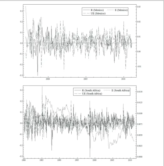
which are derived from the growth rate of consumer price indexes (CPI), as well as the GDP growth rate which is the monthly interpolated version of the quarterly GDP. We use monthly industrial production index to disaggregate this quarterly observations (see, e.g. Massimiliano Marcellino, James H. Stock, and Mark W. Watson 2003). All of the series, except the stock returns, are taken from the International Financial Statistics of the International Monetary Fund (IMF 2011). The stock returns are taken from Bolsa Mexicana De Valores (BMV 2012, Mexico2) and Johannesburg Securities Exchange (JSE 2012, South Africa3). At the end of December 2010, the market capitalisation of these stock exchanges were as follows: $749 billion, and $925 billion, respectively. The expected inflation rate is estimated with the ARFIMA (r,d,s). According to the Akaike information criteria (AIC), the ARFIMA (2,d,2) is found to be the best forecasting model for South Africa, and the ARFIMA (1,d,0) is found to be the best forecasting model for Mexico. The expected inflation is also estimated with the ARMA (r,s) models but the ARFIMA (r,d,s) was found to be the best-performing forecasting model according to AIC. The results of the ARFIMA (r,d,s) are not reported to conserve space, but are available from the author upon request. The unexpected inflation rate is estimated with the residuals obtained from the ARFIMA models. The dataset covers 170 observations from January 1997 to February 2011 for Mexico, and 374 observations from January 1980 to February 2011 for South Africa. These sample periods were chosen according to data availability. Figure 1 shows real stock returns, as well as expected and unexpected inflation.

2_{Bolsa Mexicana De Valores (BMV).}

2012. http://www.bmv.com.mx/ (accessed June 8, 2012).

3_{Johannesburg Securities Exchange (JSE). 2012.}

64 Atilla Cifter

Source: IMF (2011), BMV (2012), and JSE (2012), author’s calculation.

Figure 1 Monthly Stock Returns, Expected and Unexpected Inflation

65

Stock Returns, Inflation, and Real Activity in Developing Countries: A Markov-Switching Approach

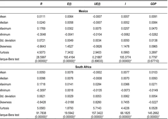
Table 2 Descriptive Statistics

R E(I) UE(I) I GDP

Mexico

Mean 0.0111 0.0064 -0.0007 0.0057 0.0091

Median 0.0240 0.0058 -0.0007 0.0052 0.0084

Maximum 0.1769 0.0302 0.0075 0.0257 0.0470

Minimum -0.3048 -0.0041 -0.0104 -0.0062 -0.0262

Std. deviation 0.0721 0.0049 0.0034 0.0050 0.0138

Skewness -0.6643 1.4527 -0.0826 1.1478 0.0965

Kurtosis 4.5073 7.3432 2.9403 6.0993 3.2697

Jarque-Bera test 28.5997 (0.00000)*

193.4164 (0.00000)*

0.21887 (0.89633)

105.3774 (0.00000)*

0.7797 (0.67710)

South Africa

Mean 0.0050 0.0078 -0.0002 0.0077 0.0103

Median 0.0098 0.0076 -0.0008 0.0070 0.0093

Maximum 0.1718 0.0141 0.0284 0.0366 0.0271

Minimum -0.3097 0.0018 -0.0135 -0.0073 -0.0149

Std. deviation 0.0621 0.0029 0.0053 0.0062 0.0054

Skewness -0.6428 -0.0188 0.8260 0.7455 -0.0227

Kurtosis 5.0583 1.8793 5.7143 4.4226 6.0528

Jarque-Bera test 91.7838 (0.00000)*

19.5942 (0.00000)*

157.3422 (0.00000)*

66.1825 (0.00000)*

145.2662 (0.00000)*

Notes: The figures in the parenthesis are p-values and denote significance at a 1% level.

Source: Author’s estimation.

66 Atilla Cifter

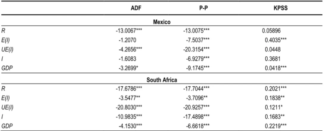
Table 3 Unit Root Test Statistics of the Time Series

ADF P-P KPSS

Mexico

R -13.0067*** -13.0075*** 0.05896

E(I) -1.2070 -7.5037*** 0.4035***

UE(I) -4.2656*** -20.3154*** 0.0448

I -1.6083 -6.9279*** 0.3681

GDP -3.2699* -9.1745*** 0.0418***

South Africa

R -17.6786*** -17.7044*** 0.2021***

E(I) -3.5477** -3.7096** 0.1838**

UE(I) -20.8030*** -20.9257*** 0.1211*

I -10.9835*** -17.4898*** 0.1683**

GDP -4.1530*** -6.6618*** 0.2219***

Notes: The number of lags (nl) in the tests has been selected using the Schwarz information criterion with a maximum of twelve lags. Test critical values are taken from MacKinnon’s one-sided p-values. *, **, *** indicate significance at the 10%, 5%, and 1%, respectively.

Source: Author’s estimation.

3.2 Empirical Findings

3.2.1 Real Stock Returns and Inflation Dynamics

67

Stock Returns, Inflation, and Real Activity in Developing Countries: A Markov-Switching Approach

Table 4 Tests for Regime-Switchinga

Ex-post analysis Ex-ante analysis

LR test LR test

Mexico 15.796

[0.0075] a

16.204 [0.0063] a

South Africa 21.695

[0.0006] a

31.696 [0.0000] a

Notes: This table shows the non-linearity tests ( 2 ) 5 (

 ). The figures in the squared brackets are upper bound p-values which are derived by Davies (1987), and a _{denote significance at a 1% level.}

Source: Author’s estimation.

Source: Author’s estimation.

68 Atilla Cifter

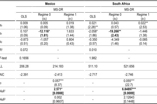
Table 5 reports the maximum likelihood estimation of the OLS and the feasi-ble sequential quadratic programming (SQPF) estimation (Craig T. Lawrence and André L. Tits 2001) of the MS-DR models for ex-post analysis. The SQPF numerical optimisation algorithm is chosen since this algorithm is more effective for non-linear time series. According to the OLS models, only the coefficient of expected inflation is statistically significant and negative for South Africa. The major drawback of all OLS models is that the f values are statistically insignificant. Consequently, the Fish-er hypothesis does not hold true for all of the countries for the OLS models because of the insignificance of f values.

Table 5 Stock Returns and Inflation (Ex-Post Analysis)

Mexico South Africa

MS-DR MS-DR

OLS Regime 0

(s0)

Regime 1

(s1) OLS

Regime 0 (s0)

Regime 1 (s1)

α0 0.009

(1.06)

0.005 (0.09)

0.019 (1.38)

0.021 (2.28)**

0.043 (0.57)

0.022** (2.53)

α1 0.107

(0.09)

-12.116* (1.81)

1.633 (1.44)

-2.058* (1.86)

-19.266** (2.43)

-1.446 (1.38)

α2 -0.873

(0.51)

-1.057 (0.20)

0.804 (0.43)

-0.350 (0.57)

-4.349 (1.46)

-0.085 (0.14)

R2 _{0.072 - 0.010 -}

F-test 0.1656 - 1.982 -

LL 206.28 214.183 511.10 521.656

AIC -2.391 -2.413 -2.717 -2.746

 - 0.057***

(8.37) -

0.055*** (22.7)

Null1 _- 2.571*

[0.0988] -

6.84897*** [0.0089]

Null2 _- 0.002

[0.9607] -

2.12643 [0.1448]

Notes:Ex-post estimates for the MS-DR models. The numbers in parentheses are the t-statistics, and the numbers in square brackets are the p-values. *, **, *** indicate significance at the 10%, 5%, and 1% level, respectively. Null1 _{refers to}

the null hypothesis of α1(s0) = α1(s1); null2 refers to the null hypothesis of α2(s0) = α2(s1).

Source: Author’s estimation.

In order to find out the regime-dependent effects of expected and unexpected inflation on real stock returns, the MS-DR model is estimated for ex-post analysis. The AIC values show that the predictive performances of the MS-DR models are higher than the OLS models. Accordingly, the MS-DR models should be chosen to find out the effect of inflation on real stock returns. Prior to analysing the coefficients in the MS-DR models, they should be tested to see whether there is a difference be-tween the expansion (s1) and the recession (s0) periods for expected and unexpected

inflation. In order to find out regime differences, two hypotheses are developed. Null1 refers to the null hypothesis of 1(s0)1(s1), and this hypothesis tests the

69

Stock Returns, Inflation, and Real Activity in Developing Countries: A Markov-Switching Approach

) ( )

( 0 2 1

2 s  s

  , and this hypothesis tests the single regime for unexpected infla-tion. The empirical results show that null1 is rejected for both Mexico and South Africa, and the rejection of 1(s0) 1(s1) indicates that there is significant regime

difference in expected inflation. Null2 hypothesis is not rejected for all of the coun-tries, and this indicates that regime difference does not exist for unexpected inflation. According to these results, it can be inferred that there is significant regime differ-ence for expected inflation. Therefore, only expected inflation coefficients can be interpreted for the ex-post analysis. Expected inflation coefficient (₁) is statistically significant only in the recession period for both Mexico and South Africa. This can be interpreted as an increase in expected inflation decreases real stock returns only in the recession period. These results show that the negative relationship between ex-pected inflation and real stock returns is regime-dependent for these two countries for

ex-post analysis. These findings should be checked for ex-ante analysis in order to find out the effect of announced inflation on real stock returns.

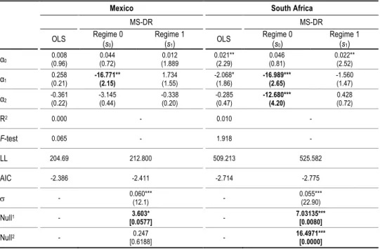
Table 6 reports the OLS and the MS-DR estimates for the ex-ante analysis. Same as ex-post analysis, only the coefficient of expected inflation is statistically significant and negative for South Africa in the OLS model. However, the f values show that all of the OLS models are statistically insignificant. Therefore, the coeffi-cients of the OLS models should not be interpreted and there is not any causality from inflation rate to real stock returns. In order to find out the regime-dependent effects of previous period expected and unexpected inflation on real stock returns, the MS-DR model is estimated for ex-ante analysis. Null of ₁(s₀)₁(s₁), and null

of ₂(s₀)₂(s₁) are also tested to find out the regime differences for ex-ante

analy-sis. Null1 is rejected for all of the countries, and the rejection of ₁(s₀)₁(s₁)

70 Atilla Cifter

Table 6 Stock Returns and Inflation (Ex-Ante Analysis)

Mexico South Africa

MS-DR MS-DR

OLS Regime 0

(s0)

Regime 1

(s1) OLS

Regime 0 (s0)

Regime 1 (s1)

α0 0.008 (0.96)

0.044 (0.72)

0.012 (1.889

0.021** (2.29)

0.046 (0.81)

0.022** (2.52)

α1 0.258 _(0.21) -16.771** _(2.15) 1.734 _(1.55) -2.068* _(1.86) -16.989*** _(2.65) -1.560 _(1.47)

α2 -0.361 (0.22)

-3.145 (0.44)

-0.338 (0.20)

-0.285 (0.47)

-12.680*** (4.20)

0.428 (0.72)

R2 _{0.000 - 0.010 -}

F-test 0.065 - 1.918 -

LL 204.69 212.800 509.213 525.582

AIC -2.386 -2.411 -2.714 -2.775

 - 0.060***

(12.1) -

0.055*** (22.90)

Null1 _- 3.603*

[0.0577] -

7.03135*** [0.0080]

Null2 _- 0.247

[0.6188] -

16.4971*** [0.0000]

Notes:Ex-ante estimates for the MS-DR models. The numbers in brackets are the t-statistics, and the numbers in squared brackets are the p-values. *, **, *** indicates significance at the 10%, 5%, and 1% level, respectively. Null1 _{refers to the null}

hypothesis of α1(s0) = α1(s1); null2 refers to the null hypothesis of α2(s0) = α2(s1).

Source: Author’s estimation.

3.2.2 Stock Returns, Inflation, and Real Activity Dynamics

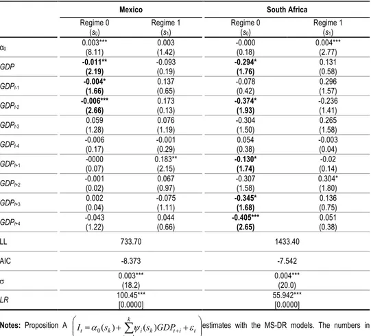
Real stock returns and inflation dynamics with the MS-DR model show that the rela-tionship between real stock returns and inflation is negative only in the recession pe-riod. Real stock returns might respond differently to inflation in a regime of the ex-pansion and the recession due to regime-dependent proxy effect hypothesis. There-fore, we test real stock returns, inflation, and real activity dynamics with Fama’s (1981) proxy effect hypothesis. In order to estimate regime differences for stock re-turns, inflation, and real activity dynamics, the regime-dependent proxy effect hypo-thesis has been developed. Same as the standard proxy effect hypohypo-thesis, the regime-dependent proxy effect hypothesis is tested with two stages: test of inflationary trends and real activity (proposition A), and test of real stock returns and real activity (proposition B).

71

Stock Returns, Inflation, and Real Activity in Developing Countries: A Markov-Switching Approach

Table 7 Inflationary Trends and Real Activity (Proposition A)

Mexico South Africa

Regime 0 (s0)

Regime 1 (s1)

Regime 0 (s0)

Regime 1 (s1)

α0 0.003***

(8.11) 0.003 (1.42) -0.000 (0.18) 0.004*** (2.77)

GDP -0.011**

(2.19) -0.093 (0.19) -0.294* (1.76) 0.131 (0.58)

GDPt-1 -0.004*

(1.66) 0.137 (0.65) -0.078 (0.42) 0.296 (1.57)

GDPt-2 -0.006***

(2.66) 0.173 (0.13) -0.374* (1.93) -0.236 (1.41)

GDPt-3 0.059

(1.28) 0.076 (1.19) -0.304 (1.50) 0.265 (1.58)

GDPt-4 -0.006

(0.17) -0.001 (0.29) 0.054 (0.38) -0.003 (0.04)

GDPt+1 -0000

(0.07) 0.183** (2.15) -0.130* (1.74) -0.02 (0.14)

GDPt+2 -0.001

(0.02) 0.067 (0.97) -0.307 (1.58) 0.304* (1.80)

GDPt+3 _(0.04) 0.002 -0.075_(1.11) -0.345*_(1.68) 0.136 _(0.75)

GDPt+4 -0.043

(1.22) 0.044 (0.66) -0.405*** (2.65) 0.051 (0.38)

LL 733.70 1433.40

AIC -8.373 -7.542

 0.003***_(18.2) 0.004***_(20.0)

LR 100.45***

[0.0000]

55.942*** [0.0000]

Notes: Proposition A

        



  t

k k i i t k i k

t s s GDP

I ₀( )  ( )  estimates with the MS-DR models. The numbers in

brackets are the t-statistics, and the numbers in squared brackets are the p-values. *, **, *** indicates significance at the 10%, 5%, and 1% level, respectively.

Source: Author’s estimation.

two lags as well as one, three, and four leads is negative and statistically significant for South Africa in the recession period. In the expansion period, neither the GDP with no leads and lags nor the GDP with up to four leads and lags are negative and statistically significant. This indicates that the regime-dependent inflationary trends and real activity (proposition A) are valid only in the recession period. Therefore, the regime-dependent proxy effect hypothesis explains the negative relationship between inflation and stock returns in the recession period for both of the countries.

72 Atilla Cifter

both of the countries only in the recession period. The GDP with one and three lags and up to two leads is positive and statistically significant for Mexico, and the GDP with one, three and four lags, and up to two leads is positive and statistically signifi-cant for South Africa in the recession period. In the expansion period, only the GDP with four leads is positive and statistically significant for Mexico. This indicates that the regime-dependent inflationary trends and real activity (proposition A) are valid only in the recession period. Nikolaos Giannellis, Angelos Kanas, and Athanasios P. Papadopoulos (2010) find that unexpected instability shocks in real activity negative-ly affects stock returns and our findings support this statement.

Table 8 Stock Returns and Real Activity (Proposition B)

Mexico South Africa

Regime 0 (s0)

Regime 1 (s1)

Regime 0 (s0)

Regime 1 (s1)

α0 -0.113***

(4.02) 0.016* (1.73) 0.002 (0.03) 0.006 (0.76)

GDP 3.061*

(1.79) 0.168 (0.18) 3.246* (1.69) 0.809 (0.39)

GDPt-1 3.719**

(2.01) -0.564 (0.68) 2.777*** (7.65) -0.004*** (0.02)

GDPt-2 -0.422

(0.15) -0.229 (0.35) 1.082 (0.16) 0.513 (0.34)

GDPt-3 4.102*

(1.67) 1.183 (1.28) 19.576*** (2.73) -0.722 (0.50)

GDPt-4 -0.940

(0.62) -0.689 (0.92) 21.893** (2.08) 1.384 (1.33)

GDPt+1 2.766***

(3.03) 2.466 (1.07) 1.059** (2.20) -1.908 (0.93)

GDPt+2 6.045***

(3.87) -1.114 (1.44) 2.681*** (5.78) -0.056 (0.02)

GDPt+3 0.296

(0.17) -0.745 (0.93) 5.608 (0.77) 2.244 (1.52)

GDPt+4 1.024

(0.84) 1.356** (2.40) 0.705 (0.10) -1.512 (1.45)

LL 222.52 527.00

AIC -2.347 -2.695

 0.048***_(12.2) 0.052***_(20.1)

LR 23.376**

[0.0247]

33.681 [0.0000]***

Notes: Proposition B

        



  t

k k i i t k i k

t s s GDP

R 0( )  ( )  estimates with the MS-DR models. The numbers in

brackets are the t-statistics, and the numbers in squared brackets are the p-values. *, **, *** indicates significance at the 10%, 5%, and 1% level, respectively.

73

Stock Returns, Inflation, and Real Activity in Developing Countries: A Markov-Switching Approach

4. Conclusion

This paper investigates the regime-dependent relationship between real stock returns, inflation, and real activity with the MS-DR approach for Mexico and South Africa. These are ideal developing countries to study this issue because they have the most attractive market capitalisation ratio for both the local and the foreign investors among other developing countries. Moreover, each of the countries represents differ-ent regions of the World, and this reduces the location bias for the analysis.

74 Atilla Cifter

References

Acker, Daniella, and Nigel W. Duck. 2013a.“Do Investors Suffer from Money Illusion? A

Direct Test of the Modigliani-Cohn Hypothesis.” Review of Finance, 17(2): 565-596.

Acker, Daniella, and Nigel W. Duck. 2013b.“Inflation Illusion and the US Dividend Yield:

Some Further Evidence.” Journal of International Money and Finance, 33(C):

235-254.

Adrangi, Bahram, Arjun Chatrath, and Todd M. Shank. 1999. “Inflation, Output, and

Stock Prices: Evidence from Latin America.” Managerial and Decision Economies,

20(2): 63-74.

Alagidede, Paul. 2009. “Relationship between Stock Returns and Inflation.” Applied

Economics Letters, 16(14): 1403-1408.

Alagidede, Paul, and Theodore Panagiotidis. 2012. “Stock Returns and Inflation: Evidence

from Quantile Regressions.” Economics Letters, 117(1): 283-286.

Ang, Andrew, Geert Bekaert, and Min Wei. 2007. “Do Macro Variables, Asset Markets, or

Surveys Forecast Inflation Better?” Journal of Monetary Economics, 54(4):

1163-1212.

Bargain, Olivier, and Prudence Kwenda. 2011. “Earnings Structures, Informal

Employment, and Self-Employment: New Evidence from Brazil, Mexico, and South

Africa.” Review of Income and Wealth, 57(Special Issue): 100-122.

Bekaert, Geert, and Eric Engstrom. 2010. “In_flation and the Stock Market: Understanding

the ‘Fed Model’.” Journal of Monetary Economics, 57(3): 278-294.

Boudoukh, Jacob, and Matthew Richardson. 1993. “Stock Returns and Inflation: A

Long-Horizon Perspective.” American Economic Review, 83(5): 1346-1355.

Campbell, John Y., and Tuomo Vuolteenaho. 2004. “Inflation Illusion and Stock Prices.”

American Economic Review, 94(2): 19-23.

Chang, Hsiao-Fen. 2013. “Are ‘Stock Returns’ a Hedge against Inflation in Japan?

Determination Using ADL Bounds Testing.” Applied Economics Letters, 20(14):

1305-1309.

Cohen, Randolph B., Christopher Polk, and Tuomo Vuolteenaho. 2005. “Money Illusion

in the Stock Market: The Modigliani-Cohn Hypothesis.” Quarterly Journal of

Economics, 120(2): 639-668.

Davies, Robert B. 1987. “Hypothesis Testing when a Nuisance Parameter Is Present only

under the Alternative.” Biometrika, 74(1): 33-43.

Dickey, David A., and Wayne A. Fuller. 1981. “Likelihood Ratio Statistics for

Autoregressive Time Series with a Unit Root.” Econometrica, 49(4): 1057-1072.

Durai, S. Raja Sethu, and Saumitra N. Bhaduri. 2009. “Stock Prices, Inflation and Output:

Evidence from Wavelet Analysis.” Economic Modelling, 26(5): 1089-1092.

Engsted, Tom, and Carsten Tanggaard. 2002. “The Relation between Asset Returns and

Inflation at Short and Long Horizons.” Journal of International Financial Markets,

Institutions and Money, 12(2): 101-118.

Erb, Claude B., Campbell R. Harvey, and Tadas E. Viskanta. 1995. “Inflation and World

Equity Selection.” Financial Analysts Journal, 51(6): 28-42.

Fama, Eugene F., and G. William Schwert. 1977. “Asset Returns and Inflation.” Journal of

Financial Economics, 5(2): 115-146.

Fama, Eugene F. 1981. “Stock Returns, Real Activity, Inflation, and Money.” American

75

Stock Returns, Inflation, and Real Activity in Developing Countries: A Markov-Switching Approach

Fisher, Irving. 1930. The Theory of Interest, as Determined by Impatience to Spend Income

and Opportunity to Invest It. New York: Macmillan Publishers.

Frühwirth-Schnatter, Sylvia. 2006. Finite Mixture and Markov Switching Models. New

York: Springer.

Giannellis, Nikolaos, Angelos Kanas, and Athanasios P. Papadopoulos. 2010.

“Asymmetric Volatility Spillovers between Stock Market and Real Activity: Evidence

from the UK and the US.” Panoeconomicus, 57(4): 429-445.

Giordani, Paolo, and Paul Söderlind. 2003. “Inflation Forecast Uncertainty.” European

Economic Review, 47(6): 1037-1059.

Gultekin, N. Bulent. 1983. “Stock Market Returns and Inflation: Evidence from Other

Countries.” Journal of Finance, 38(1): 49-65.

Hamilton, James D. 1989. “A New Approach to the Economic Analysis of Nonstationary

Time Series and the Business Cycle.” Econometrica, 57(2): 357-384.

Hasan, Mohammad S. 2008. “Stock Returns, Inflation and Interest Rates in the United

Kingdom.” European Journal of Finance, 14(8): 687-699.

Hondroyiannis, George, and Evangelia Papapetrou. 2006. “Stock Returns and Inflation in

Greece: A Markov Switching Approach.” Review of Financial Economics, 15(1):

76-94.

Hong, Gwangheon, Jaeuk Khil, and Bong-Soo Lee. 2013. “Stock Returns, Housing Returns

and Inflation: Is there an Inflation Illusion?” Asia-Pacific Journal of Financial Studies,

42(4): 511-562.

Hsing, Yu, and Wen-jen Hsieh. 2012. “Impacts of Macroeconomic Variables on the Stock

Market Index in Poland: New Evidence.” Journal of Business Economics and

Management, 13(2): 334-343.

Karagianni, Stella, and Catherine Kyrtsou. 2011. “Analysing the Dynamics between U.S.

Inflation and Dow Jones Index Using Non-Linear Methods.” Studies in Nonlinear

Dynamics and Econometrics, 15(2): 1-25.

Khil, Jaeuk, and Bong-Soo Lee. 2000. “Are Common Stocks a Good Hedge against

Inflation? Evidence from the Pasific-rim Countries.” Pasific-Basin Finance Journal,

8(3-4): 457-482.

Knif, Johan, James Kolari, and Seppo Pynnönen. 2008. “Stock Market Reaction to Good

and Bad Inflation News.” Journal of Financial Research, 31(2): 141-166.

Koustas, Zisimos, and Apostolos Serletis. 1999. “On the Fisher Effect.” Journal of

Monetary Economics, 44(1): 105-130.

Kwiatkowski, Denis, Peter C. B. Phillips, Peter Schmidt, and Yongcheol Shin. 1992.

“Testing the Null Hypothesis of Stationarity against the Alternative of a Unit Root:

How Sure Are We that Economic Time Series Have a Unit Root?” Journal of

Econometrics, 54(1-3): 159-178.

Lawrence, Craig T., and André L. Tits. 2001. “A Computationally Efficient Feasible

Sequential Quadratic Programming Algorithm.” SIAM Journal on Optimization,11(4):

1092-1118.

Lawrence, Kryzanowski, and Abdul H. Rahman. 2009. “Generalized Fama Proxy

Hypothesis: Impact of Shocks on Phillips Curve and Relation of Stock

Returns with Inflation.” Economics Letters, 103(3): 135-137.

Lee, Keun Yeong. 2008. “Causal Relationships between Stock Returns and Inflation.”

76 Atilla Cifter

Li, Lifang, Paresh K. Narayan, and Xinwei Zheng. 2010. “An Analysis of Inflation and

Stock Returns for the UK.” Journal of International Financial Markets, Institutions

and Money, 20(5): 519-532.

Lin, Shu-Chin. 2009. “Inflation and Real Stock Returns Revisited.” Economic Inquiry, 47(4):

783-795.

Luintel, Kul B., and Krishna Paudyal. 2006. “Are Common Stocks a Hedge against

Inflation?” Journal of Financial Research, 29(1): 1-19.

Madsen, Jakob B., Ratbek Dzhumashev, and Hui Yao. 2013. “Stock Returns and

Economic Growth.” Applied Economics, 45(10): 1257-1271.

Marcellino, Massimiliano, James H. Stock, and Mark W. Watson. 2003. “Macroeconomic

Forecasting in the Euro Area: Country Specific versus Area-Wide Information.”

European Economic Review, 47(1): 1-18.

Mitchell-Innes, Henry A., Meshach J. Aziakpono, and Alexander P. Faure. 2007.

“Inflation Targeting and the Fisher Effect in South Africa: An Empirical

Investigation.” South African Journal of Economics, 75(4): 693-707.

Mitra, Sharmishtra, Basab Nandi, and Amit Mitra. 2007. “Study of Dynamic

Relationships between Financial and Real Sectors of Economies with Wavelets.”

Applied Mathematics and Computation, 188(1): 83-95.

Modigliani, Franco, and Richard A. Cohn. 1979. “Inflation, Rational Valuation, and the

Market.” Financial Analysts Journal, 35(2): 24-44.

Mundell, Robert. 1963. “Inflation and Real Interest Rates.” Journal of Political Economy,

71(3): 280-283.

Oxman, Jeffrey. 2012. “Price Inflation and Stock Returns.” Economics Letters, 116(3):

385-388.

Ozdemir, Zeynel A., and Mahir Fisunoglu. 2008. “On the Inflation-Uncertainty Hypothesis

in Jordan, Philippines and Turkey: A Long Memory Approach.” International Review

of Economics and Finance, 17(1): 1-12.

Philippon, Thomas. 2009. “The Bond Market’s q.” Quarterly Journal of Economics, 124(3):

1011-1056.

Phillips, Peter C. B., and Pierre Perron. 1988. “Testing for a Unit Root in Time Series

Regression.” Biometrika, 75(2): 335-346.

Rapach, David E. 2002. “The Long-Run Relationship between Inflation and Real Stock

Prices.” Journal of Macroeconomics, 24(3): 331-351.

Rushdi, Mustabshira, Jae H. Kim, and Param Silvapulle. 2012. “ARDL Bounds Tests and

Robust Inference for the Long Run Relationship between Real Stock Returns and

Inflation in Australia.” Economic Modelling, 29(3): 535-543.

Ryan, Geraldine. 2006. “Irish Stock Returns and Inflation: A Long Span Perspective.”

Applied Financial Economics, 16(9): 699-706.

Schmeling, Maik, and Andreas Schrimpf. 2011. “Expected Inflation, Expected Stock

Returns, and Money Illusion: What Can We Learn from Survey Expectations?”

European Economic Review, 55(5): 702-719.

Schwert, G. William. 1981. “The Adjustment of Stock Prices to Information about Inflation.”

Journal of Finance, 36(1): 15-29.

Solnik, Bruno. 1983. “The Relation between the Stock Prices and Inflationary Expectations:

The International Evidence.” Journal of Finance, 38(1): 35-48.

Wei, Chao. 2009. “Does the Stock Market React to Unexpected Inflation Differently across