Elections and stock market volatility: evidence in OECD countries and developing countries

(1)

FUNDAÇÃO GETÚLIO VARGAS

ESCOLA DE ECONOMIA DE EMPRESAS DE SÃO PAULO

JOÃO MENDES

Elections and Stock Market Volatility: Evidence in OECD countries and Developing countries

(2)

FUNDAÇÃO GETÚLIO VARGAS

ESCOLA DE ECONOMIA DE EMPRESAS DE SÃO PAULO

JOÃO MENDES

SÃO PAULO 2015

Dissertação apresentada à Escola de Economia de Empresas de São Paulo da

Fundação Getúlio Vargas, como

requisito para obtenção do título de Mestre Profissional em Economia.

Campo do Conhecimento: International Master in Finance

(3)

Mendes, João.

Elections and Stock Market Volatility: Evidence in OECD countries and Developing countries / João Mendes. - 2015.

53 f.

Orientador: João de Mendonça Mergulhão.

Dissertação (MPFE) - Escola de Economia de São Paulo.

1. Mercado de capitais. 2. Ações (Finanças). 3. Eleições. I. Mergulhão, João de Mendonça. II. Dissertação (MPFE) - Escola de Economia de São Paulo. III. Título.

(4)

JOÃO MENDES

Dissertação apresentada à Escola de Economia de Empresas de São Paulo da Fundação Getúlio Vargas, como requisito para obtenção do título de Mestre Profissional em Economia.

Campo do Conhecimento: International Master in Finance

Data de Aprovação: 24/ 09/ 2015

Banca Examinadora:

_________________________________ Prof. Dr. João de Mendonça Mergulhão (ADVISOR)

_________________________________

Prof. Dr. Luís Brites Pereira

(DISCUSSANT)

(5)

Acknowledgements

The final stage of this Master Project is coming to an end. The time spent in

Lisbon, London and São Paulo gave me the chance of experiencing different approaches

to several problems. This final report is now finished, but it would not be possible to

make it happen without the help and support of those near me.

I would like to first acknowledge the help of my supervisors. Their insightful

observations and availability made this work possible. To Professor Doutor Luis Brites

Pereira and Professor Doutor João de Mendonça Mergulhão, my deepest thanks.

I would like also to express my thanks to all the Professors in Lisbon and São

Paulo which I had the privilege of knowing and with whom I learned many interesting

subjects.

To my family. Without their support this task would have not have been

possible. I want to deeply thank all my grandparents, specially my grandfather

“Manecas” that was essential in this step. To my uncle Francisco who had a key role in

the last stage of this Master. And of course, my Dad, my Mum, my sister and my

brother that gave me the support I needed in all moments of this path.

To my friends, Lourenço, Rita and Pedro that, in Portugal, always paid attention

to what was happening in São Paulo. It was very important.

Finally, a special word for my friend Ricardo that, with his patient, played a very

important role for the achievement of this objective.

To all of you, thank you,

(6)

Resumo

Este trabalho estuda se existe impacto na volatilidade dos mercados de ações em

torno das eleições nacionais nos países da OCDE e nos países em Desenvolvimento. Ao

mesmo tempo, pretende, através de variáveis explicativas, descobrir os fatores

responsáveis por esse impacto. Foi descoberta evidência que o impacto das eleições na

volatilidade dos mercados de ações é maior nos países em Desenvolvimento. Enquanto

as eleições antecipadas, a mudança na orientação política e o tamanho da população

foram os factores que explicaram o aumento da volatilidade nos países da OCDE, o

nível democrático, número de partidos da coligação governamental e a idade dos

mercados foram os factores explicativos para os países em Desenvolvimento.

(7)

Abstract

This project studies whether there is impact in stock market volatility around

national elections in OECD countries and Developing countries. At the same time, it

pretends, through a set of explanatory variables, find the factors that are responsible for

that impact. It was found evidence that the impact of elections in stock market volatility

is bigger in Developing countries. While early elections, the change in political

orientation and the size of population were the factors that explained the abnormal

volatility in OECD countries, the level of democracy, the number of parties of the

governmental coalition and the age of the stock markets were the ones for Developing

countries.

(8)

List of Tables

Table 1 - Sample composition for OECD countries ... 18

Table 2 - Sample composition for Developing countries ... 19

Table 3 - Descriptive Statistics for OECD countries ... 22

Table 4 - Descriptive Statistics for Developing countries ... 22

Table 5 - Descriptive Statistics for the new variables included for Developing countries ... 24

Table 6 - Cumulative Abnormal Volatility around Election Day (2002-2014): OECD vs Developing countries ... 26

Table 7 – Test for CAV differences between Developing and OECD countries ... 27

Table 8 - Cumulative abnormal volatility around Election Day on OECD countries: 1982-2004 vs 2002-2014 ... 28

Table 9 - ANOVA for OECD countries after treatment ... 30

Table 10 - Coefficients for OECD countries after treatment ... 30

Table 11 - ANOVA for Developing countries after treatment ... 31

Table 12 - Coefficients for Developing countries after treatment ... 31

Table 13 – Election dates in OECD countries ... 40

Table 14 – Election dates in Developing countries ... 40

Table 15 – Minority Government in OECD countries ... 41

Table 16 – Minority Government in Developing countries ... 41

Table 17 – Margin of Victory in OECD countries ... 42

Table 18 – Margin of Victory in Developing countries ... 42

Table 19 – Number of Parties in OECD countries ... 43

Table 20 – Number of Parties in Developing countries ... 43

Table 21 – Change in Orientation in OECD countries ... 44

Table 22 – Change in Orientation in Developing countries ... 44

Table 23 – Early Election in OECD countries ... 45

Table 24 – Early Election in Developing countries ... 45

Table 25 – Age in OECD countries ... 46

Table 26 – Compulsory in OECD countries ... 46

Table 27 – Age in Developing countries ... 46

Table 28 – Compulsory in Developing countries ... 46

Table 29 – Population in OECD countries ... 47

Table 30 – Population in Developing countries ... 47

Table 31 – GDP per capita in OECD countries... 48

Table 32 – GDP per capita in Developing countries ... 48

Table 33 – Democracy in Developing countries ... 49

Table 34 – KOF index in Developing countries ... 49

Table 35 – Development in Developing countries ... 49

Table 36 - Correlation matrix for OECD countries ... 50

Table 37 - Correlation matrix for Developing countries ... 51

Table 38 - ANOVA for OECD countries ... 52

Table 39 - Coefficients for OECD countries ... 52

Table 40 - ANOVA for Developing countries ... 52

(10)

10

Introduction

National elections represent the major moment when population choose the

people who represent them in the making of economic, political and social decisions.

This choice will strongly influence the path each country will take.

Political events have a big influence in financial markets because markets tend

to respond to new information regarding political decisions that can impact on monetary

and fiscal policy. The perception that the outcome of the elections influences the

movement of stock markets has been an evidence in the social media both in

Organisation for Economic Co-operation and Development (OECD) countries and in

Developing countries.

An example is the newspaper´s “El País” quote regarding Brazilian

Presidential elections in October 2014: “As might be expected, the market reacted badly to the re-election of President Dilma Rousseff ... the stock market rose in fall of 6% ... the dollar advanced 3,46 % ... the Petrobras shares had registered a fall of about 13 %. It was not expected anything different from this.", says Alex Agostini , an analyst at

Austin Brokerage.”1

In the USA after Obama´s reelection in 2012, Infowars published: “Stock

markets responded to Obama’s re-election by plunging today. The Dow tumbled below

13,000 as the S&P broke 1,400, beating this year’s drop on June 1”.

The investors revise their expectations taking into account the elections outcome

depending on their profit expectations related to the elections results. Basically, the

1

(11)

11 price of a stock is related to the profits that the companies will distribute to its

shareholders (fiscal policy has influence) and the expected interest rate (monetary

policy has influence).

For example, one may say that historically it can be seen that typically the

left-wing governments tend to implement higher taxes in order to distribute more money

through social politics. Obviously, if the tax rate of the companies increases, the profit

that will be distributed as dividends for shareholders will be lower, in the same

conditions. This means that the stock price will decrease as a response to an Election of

a Government that has this political agenda as the expected dividend is lower.

All over the world there are different political systems and regimes that differ

the way the countries choose their representatives. Although there are several different

realities, in this project it will be just considered only two political systems: the

Parliamentary and the Presidential. The different political systems in each country will

be classified accordingly these two systems, neglecting small and non-significant

differences.

The Parliamentary system has the Prime Minister or Premier as the Head of

Government and the President being merely a High Representative of the State with no

executive power. In the Presidential system the President holds the position of both

Head of State and Head of Government (Executive and Representative Powers).

The present study tries to deepen the relationship between Elections and

Volatility of the stock markets and prove the perception demonstrated above.

In this project we will complement the results obtained by (Bialkowski,

(12)

12 countries were used to provide evidence that stock market volatility is substantially

raised around national elections.

This work makes the same approach for the elections occurred between 2002

and 2014 in OECD countries covering 105 elections over 32 countries. The same

analysis was extended for 13 Developing countries covering 38 elections to understand

if there is any significant impact in this group of countries as well. A comparison of the

results of these two groups of countries is done in order to understand if the national

elections have bigger impact in OECD countries or in Developing countries.

In order to provide further information regarding the factors that can influence

the magnitude of election shocks several explanatory variables were used, namely:

Parliamentary, Minority Government, Margin of Victory, Number of Parties, Orientation, Early Election, Age, Compulsory Voting, Population and GDP (Gross

Domestic Product) per Capita. The last two variables are considered in its natural

logarithm form.

These variables were used to find results for OECD countries and Developing

countries. However, for Developing countries three more variables were implemented in

the model: Democracy, Development and Globalization following the argument used by

(13)

13

Literature Review

Stock market volatility has been frequently studied regarding the way it can be

measured as well as the drivers responsible for the existence of that volatility.

For instance, (Shiller, 1981) defends that volatility does not follow the

predictions of present value models and (Grossman & Shiller, 1981) showed that the

intertemporal variation appears to be inexplicably high and cannot be rationalized even

in a model of stochastic discount factor. More recently, in his book (Wisniewski, 2009)

documented the same results as the authors mentioned before.

Financial economists faced a challenge since the fluctuation of stock markets

could not be explained by standard valuation models. Dividends and earnings are

drivers of volatility but other drivers needed to be found in order to explain the volatility

present in the stock markets. In his work, (Schwert, 1989) examined empirically how

stock return variability are linked to macroeconomic variables, financial leverage and

trading volume. His analysis indicates that only a small proportion of fluctuations in the

stock market can be explained.

The economists understood that political events may be one factor that

influences the market movements and because of this, the issue of political events that

ties to financial market performance has been the subject of several studies, e. g., in the

US, the link between political issues and economic performance was analyzed by

(Goodell & Vahamaa, 2013) and the author concluded that the presidential election

process engenders market anxiety as investors form their expectations regarding future

(14)

14 examined the market reactions to election polls. This study concluded that the changes

on election polls induced volatility in stock markets.

Furthermore, (Fuss & Bechtel, 2008) studied the effect of the expected

partisanship in the 2002 German election and found that the expectations of right or left

wings victory make the volatility of the market change. This study reinforces the idea of

the impact of political events on stock market volatility.

The studies mentioned before focused their studies in one country however, in

the paper by (Pantzalis, Stangeland, & Turtle, 2000) the authors went further realizing

that the positive reaction of the stock market to elections is shown to be a function of a

country´s degree of political, economic and press freedom, and a function of the

election timing and the success of the incumbent in being re-elected.

There are several studies with different approaches that confirm the relationship

between politics and stock market volatility. In the paper by (Bialkowski, Gottschalk, &

Wisniewski, 2008) the authors proceed to show that, in OECD countries, stock markets

can become very unsettled during periods of important political changes. In this paper it

is demonstrated that National Elections affect the stock market volatility in the days that

surround the Election Day. Apart from these results, the authors found that markets with

short trading history exhibit stronger reaction.

This project contributes to the existent literature by providing comparative study

between Developing countries and OECD countries regarding the impact of National

Elections. Finally, using a linear regression methodology, it is given information about

(15)

15

Methodology

As methodology it will be measured the impact of elections on the second

moment of return distribution using the volatility event study approach. First, it is

isolated the country-specific component of variance within a GARCH (1,1) framework:

(1)

(2)

where and are the continuously compounded returns on the US dollar

denominated stock market index in country i and the global stock market index on day t,

respectively. Also denotes the country specific part of index returns, and stands

for its conditional variance. It will be assumed that has a normal distribution with

null mean value and variance .

Equations (1) and (2) are estimated jointly using the Maximum Likelihood

method over a period immediately preceding the event window. The convention is to

use 250 days to estimate the benchmark model. However, in this work it is used 500

days because for GARCH models one year of data may be insufficient.

To measure possible abnormal volatility, one has to consider the variation in

around the event date in relation to its regular non-event level. The GARCH model may

serve as a benchmark since it can provide an indication of what the volatility would

have been, had the election not occurred.

As it stands, (2) is one-step-ahead forecast and will not generate an event

independent projection. The immediate impact of an election, as measured by will

(16)

16 volatility forecast conditional only on the information set available prior to the event.

For this reason, the volatility benchmark for k-th day of the event window is defined as

k-step-ahead forecast of the conditional variance based on the information set available

on the last day of the estimation window , with expectation given by:

(3)

The distribution of the residuals during the event window can be described as

~ N (ARt, Mt.E [ , where Mt is the multiplicative effect of the event on

volatility, ARt is the event-induced abnormal return, and t > t*. Under the null

hypothesis that investors are not surprised by elections outcomes, the value of parameter

Mt should equal one. Note that, if the residuals were demeaned using the cross-section

average, they would be normally distributed with zero mean. Since the objective of the

study is to quantify the effect of elections on stock market volatility, Mt is the parameter

of primary interest.

The method of estimating this event induced volatility multiple rests on

combining residual standardization with a cross sectional approach in the spirit of

(Boehmer, Masumeci, & Poulsen, 1991) and (Hilliard & Savickas, 2002). Note that the

estimate of Mt can be calculated as the cross-sectional variance of demeaned residuals,

standardized by the event-independent demeaned residual standard deviation, given by

(17)

17 Under the null hypothesis, the demeaned standardized residuals follow a

standard normal distribution because Mt equals one. Consequently, the abnormal

percentage change in volatility on a given day t of the event window is expressed by

. For an event window , the Cumulative Abnormal Volatility (CAV)

can be determined by:

(5)

In the current setting, the null hypothesis of no impact can be rewritten as:

, (6)

which is equivalent to

. (7)

Since, under the null hypothesis, is a variance of independent

random variables, and . The

test statistic for the hypothesis stated in (6) is therefore given by:

(8)

The inferences based on the theoretical statistic will not be robust if the

assumptions of the underlying econometric model are violated. Potential complications

may arise from non-normality, cross-sectional dependence, or autocorrelation of the

(18)

18

Data

In what follows, several computations had to be made, using a set of software,

according to the specific objective at each stage. In the Appendix 2 the functions created

for these computations are included.

This work compiled information from 105 elections in 32 industrialized

countries and from 38 elections in 13 considered as developing countries. Regarding the

industrialized countries, the work includes all OECD countries except Slovakia and

South Korea. As of the time of writing this work, Morgan Stanley Capital International

Inc. (MSCI) did not provide enough data from these two stock markets.

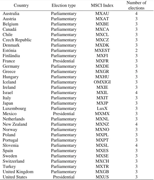
Table 1 - Sample composition for OECD countries

Country Election type MSCI Index Number of elections

Australia Parliamentary MXAU 4

Austria Parliamentary MXAT 3

Belgium Parliamentary MXBE 3

Canadá Parliamentary MXCA 3

Chile Parliamentary MXCL 3

Czech Republic Parliamentary MXCZ 3

Denmark Parliamentary MXDK 3

Estónia Parliamentary MXEST 2

Finlândia Parliamentary MXFI 3

France Presidential MXFR 3

Germany Parliamentary MXDE 3

Greece Parliamentary MXGR 5

Hungary Parliamentary MXHU 3

Iceland Parliamentary OMXIGI 3

Ireland Parliamentary MXIE 3

Israel Parliamentary MXIL 4

Italy Parliamentary MXIT 3

Japan Parliamentary MXJP 3

Luxembourg Parliamentary LuxX 3

Mexico Presidential MXMX 3

Netherlands Parliamentary MXNL 3 New Zealand Parliamentary MXNZ 4

Norway Parliamentary MXNO 3

Poland Parliamentary MXPL 3

Portugal Parliamentary MXPT 3

Slovenia Parliamentary MXSL 4

Spain Parliamentary MXES 3

Sweden Parliamentary MXSE 3

Switzerland Parliamentary MXCH 3

Turkey Parliamentary MXTR 3

(19)

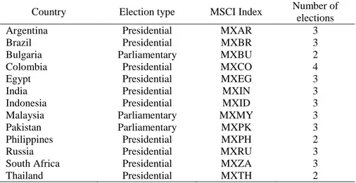
19 Table 1 and Table 2 show the election type, the MSCI Index and the number of

elections analyzed in each country.

Table 2 - Sample composition for Developing countries

Country Election type MSCI Index Number of elections

Argentina Presidential MXAR 3

Brazil Presidential MXBR 3

Bulgaria Parliamentary MXBU 2

Colombia Presidential MXCO 4

Egypt Presidential MXEG 3

India Presidential MXIN 3

Indonesia Presidential MXID 3

Malaysia Parliamentary MXMY 3

Pakistan Parliamentary MXPK 3

Philippines Presidential MXPH 2

Russia Presidential MXRU 3

South Africa Presidential MXZA 3

Thailand Presidential MXTH 2

The returns for the remaining countries were computed using US dollar

denominated MSCI Country Indices. These are value-weighted and adjusted for

dividend payments. It was chosen MSCI World Index, which measures the performance

of all developed equity markets, as a proxy for our global portfolio.

Since the objective of this work is to study the volatility around those elections

that determine the formation of national governments, we have to focus on presidential

elections in presidential systems and parliamentary elections in parliamentary systems.

Elections dates were mostly obtained by searching in each country governmental

websites. The double checking of this data was made using alternative websites.

Elections that took place 500 days after 01/01/2000 were excluded in order to be

possible to use 500 days as benchmark. This restriction enables us to estimate the

(20)

20 this, although the observations start in 2000, in this work, only the elections from 2002

until 2014 were taken into account.

In order to find the determinants of election-induced volatility it was used a

comprehensive data set of explanatory variables. These variables are supposed to

provide further information regarding political, institutional and socio-economic factors

that can influence the magnitude of the impact around Election Day.

The following explanatory variables were used for both OECD countries and

Developing countries:

 Parliamentary: dummy variable that signals the difference between

parliamentary and presidential systems. It takes the value of 1 when it is

parliamentary system and 0 otherwise.

 Minority Government: dummy variable that indicates when a minority

government is brought to office, i. e., when in a parliamentary system the

majority of seats was not achieved in the election and it was not made a coalition

to provide it. In the presidential systems the majority is always obtained. This

variable assumes 0 in case of majority and 1 in case of minority.

 Margin of Victory: it is the difference between the election winners and the

opposition. In parliamentary systems can be the difference between the

government coalition and all the other parties, whereas on Presidential Elections

it is the difference between the winner and the runner-up.

 Number of Parties: indicates the number of independent parties involved in the

government coalition for parliamentary systems. It takes the value of 1 for

(21)

21

 Orientation: dummy variable that tends to show shifts in political orientation.

This means when there is a shift from left wing to right wing or vice-versa. The

classification of left or right wing is not entirely uncontroversial and may be

deemed somewhat subjective, therefore it was followed the conventions adopted

by (Banks, Muller, & Overstreet, 2004). This variable assumes the value of 1

when there is a change in political orientation.

 Early Election: dummy variable that indicates when an election is called, at

least, three months before the official end of the mandate that was in course. It

takes the value of 1 when the election is called early and 0 otherwise.

 Age: dummy variable that takes the value of 1 when the stock market of that

country was established after 1860 and 0 when established before the same date.

 Compulsory Voting: dummy variable that assumes the value of 1 when a country

has mandatory voting laws and 0 otherwise.

 Ln (Population): is the natural logarithm of the total population in a given

country-year.

 Ln (GDP per Capita): it is the natural logarithm of GDP per capita of the

country in the year of the elections analyzed. This value is measured in constant

2000 US dollars.

While computing these variables, different awareness levels of each of the 45

country reality was needed. For instance, variable Age, Compulsory Voting and

Parliamentary were computed with the analysis of each country by itself, while the

other considered variables implied an exhaustive search and analysis for each of the 143

elections for all countries. Not only the election by itself but also the change induced by

(22)

22

Orientation, Early Election, Ln (Population) and Ln (GDP per Capita). The

information about all variables and their computation is summarized in the Appendix.

Table 3 - Descriptive Statistics for OECD countries

Mean Standard deviation

25th

Percentile Median

75th Percentile Parliamentary 0,9109 0,2863 1,0000 1,0000 1,0000 Minority_Government 0,0737 0,2626 0,0000 0,0000 0,0000 Margin_of_Victory -0,0025 0,1636 -0,0945 -0,0146 0,0533 Number_of_Parties 2,3579 1,3599 1,0000 2,0000 3,0000 Orientation 0,5102 0,5025 0,0000 1,0000 1,0000 Early_Election 0,2857 0,4541 0,0000 0,0000 1,0000 Compulsory_Voting 0,2059 0,4104 0,0000 0,0000 0,0000

Age 0,5313 0,5070 0,0000 1,0000 1,0000

Ln_Population 16,3426 1,5801 15,5012 16,1703 17,5479 Ln_GDP_per_capita 10,3768 0,6397 10,0474 10,5418 10,7937

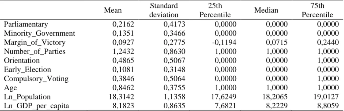
Table 4 - Descriptive Statistics for Developing countries

25th

Percentile Median

75th Percentile Parliamentary 0,2162 0,4173 0,0000 0,0000 0,0000 Minority_Government 0,1351 0,3466 0,0000 0,0000 0,0000 Margin_of_Victory 0,0927 0,2775 -0,1194 0,0715 0,2440 Number_of_Parties 1,2432 0,8630 1,0000 1,0000 1,0000 Orientation 0,4865 0,5067 0,0000 0,0000 1,0000 Early_Election 0,1081 0,3148 0,0000 0,0000 0,0000 Compulsory_Voting 0,3846 0,5064 0,0000 0,0000 1,0000

Age 0,8462 0,3755 1,0000 1,0000 1,0000

Ln_Population 18,3142 1,1358 17,6249 18,2065 19,0127 Ln_GDP_per_capita 8,1823 0,8635 7,6821 8,2229 8,8059

The information for Compulsory Voting (dummy variable) comes from an archive

of the International Institute for Democracy and Electoral Assistance (IDEA, 2015).

In the last two variables the log transformation is applied to reduce skewness in the

underlying data, as usual used when analyzing these variables under linearity condition.

Furthermore, these two variables were obtained from the database compiled by the

(23)

23 European Statistics website (EuroStat, 2015), the governmental website of each country

and confirmed with an exhaustive research on the internet.

As mentioned before, this work pretends to compare the impact of national

elections on stock markets on OECD countries and Developing countries. For these last

group of countries, and following (Macedo, Pereira, & Jalles, 2013) one can see that

there are more variables that should be accounted for and might have an impact on stock

markets: the three explanatory variables are Democracy, Development and

Globalization. The necessary computation of each variable was made comprising the

data collection taking into account each election date.

The variables are constructed as follows:

 Democracy: is the average of the two measures of the quality of democracy

published by the Freedom House: Political Rights and Civil Liberties (House,

2015), where 7 stands for minimum political rights and 1 stands for maximum

Political Rights. This scale is also used for Civil Liberties.

 Globalization: is given by the KOF index (Konjunkturforschungsstelle in

German) which measures the global connectivity, integration and

interdependence in the economic, social, technological, cultural, political, and

ecological spheres (KOF, 2015), where 100 stands for maximum globalization

and 1 stands for minimum globalization.

(24)

24 Table 5 - Descriptive Statistics for the new variables included for Developing countries

25th

Percentile Median

75th Percentile Democracy 3,4474 1,3244 2,1250 3,2500 4,5000 Globalization 59,8844 7,4714 56,3340 59,2237 63,9651 Development 0,1005 0,0697 0,0452 0,0830 0,1380

In Table 3, Table 4 and Table 5 are presented descriptive statistics for the

explanatory variables analyzed for OECD countries and Developing countries,

respectively. On Table 3 it is shown that parliamentary elections represent 91% of the

sample and only in 7% of the cases the government is formed based on a minority of

seats in the parliament. A possible explanation for the negative margin of victory in the

OECD countries is that most countries incorporated majoritarian elements in their

electoral systems. This means that with less than half of the votes it is possible to get a

majority in the parliament. An example is Greece that attributes automatically 50 seats

(out of 300) to the party or coalition that obtains more votes on the election.

As shown in Table 4, relating to Developing countries, parliamentary elections

only represent around one fourth of the elections. This is the reason why the Number of

Parties is approximately 1. Therefore, also may explain the margin of victory is positive

because usually in Presidential elections it is needed more than 50% of the votes to elect

the President.

In OECD countries, in 51% of the cases occurred a change in orientation which

is almost the same as in Developing countries. However, when compared with the data

from 1980 to 2004 presented in (Bialkowski, Gottschalk, & Wisniewski, 2008), in

OECD countries the change in orientation increased. A possible explanation for this

(25)

25 economic growth and people expect that from changing the political orientation of the

government may result in a consistent economic growth.

In developing countries only 10% of the elections are called early. The variable

Democracy has a mean of 3,44 which is too far from one which represents the most

democratic country. Another important result is that, on average, the GDP per capita of

the Developing countries is 10% of that of the US making clear the colossal economic

difference between these countries and the US, see Table 5.

When analyzing the question of compulsory voting, seven of the OECD

countries (20%) and five of Developing countries (38%) have mandatory voting laws

but stringency and enforcement of these laws appear to be country specific.

The German stock is the oldest in the sample (1585) and half of OECD countries

established its stock market before 1860. Not surprisingly, in 84% of Developing

countries the stock markets were established after 1860.

Regarding population, in OECD countries the range is 311 566 in Iceland in

2007 and 313 873 685 in the USA in 2012 whereas in Developing countries the range is

from 7 265 115 in Bulgaria in 2013 to 1 267 401 849 in India in 2014.

Finally, the range of GDP per capita is between 3 576$ in Turkey in 2002 and

110 664$ in Luxembourg in 2013 in OECD countries, while in Developing countries

the range is from 483$ in Pakistan in 2002 to 13 693$ in Argentina in 2011. These data

(26)

26

Results

The investigation starts with the volatility event study described in the

methodology section. The Election Day was defined as the event day, except for

instances when elections took place during the weekend or on a holiday. In these cases,

day zero is defined as the first trading day after the election. There are situations, as in

France and Brazil, where can happen a second round of the election and so there are two

different dates for the elections. In these situations the event day was considered the day

of the second round election.

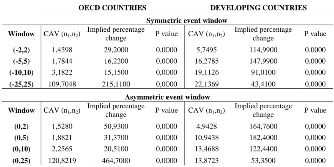
Table 6 - Cumulative Abnormal Volatility around Election Day (2002-2014): OECD vs Developing countries

OECD COUNTRIES DEVELOPING COUNTRIES

Symmetric event window

Window CAV (n1,n2)

Implied percentage

change P value CAV (n1,n2)

Implied percentage

change P value

(-2,2) 1,4598 29,2000 0,0000 5,7495 114,9900 0,0000

(-5,5) 1,7844 16,2200 0,0000 16,2785 147,9900 0,0000

(-10,10) 3,1822 15,1500 0,0000 19,1126 91,0100 0,0000

(-25,25) 109,7048 215,1100 0,0000 22,1369 43,4100 0,0000

Asymmetric event window

Implied percentage

change P value

(0,2) 1,5280 50,9300 0,0000 4,9428 164,7600 0,0000

(0,5) 1,8821 31,3700 0,0000 10,9438 182,4000 0,0000

(0,10) 2,2565 20,5100 0,0000 13,4688 122,4400 0,0000

(0,25) 120,8219 464,7000 0,0000 13,8723 53,3500 0,0000

It can be seen that in Developing countries, for example, CAV (-25,25) reaches a

value of 22,14. It is possible to realize that the ratio of CAV to the total number of days

included in the event window is, by construction, equal to the percentage increase of the

(27)

27 elections, the country-specific component of variance was 43,41% higher than it would

have been, had the elections not occurred.

Narrowing the event window tend to larger implied percentage changes,

confirming that most of the large stock market moves are concentrated around the

Election Day. An important note to consider is that around national elections the

country specific return volatility can easily double in the week of elections in

Developing countries while in OECD countries it does not happen with the same

magnitude.

Is of interest to test if the differences reported in Table 6 are statistically

significant, i.e.,

.

In Table 7 the results for the hypothesis testing are displayed, under the

assumption of the normal distribution of the test statistics.

Table 7 – Test for CAV differences between Developing and OECD countries

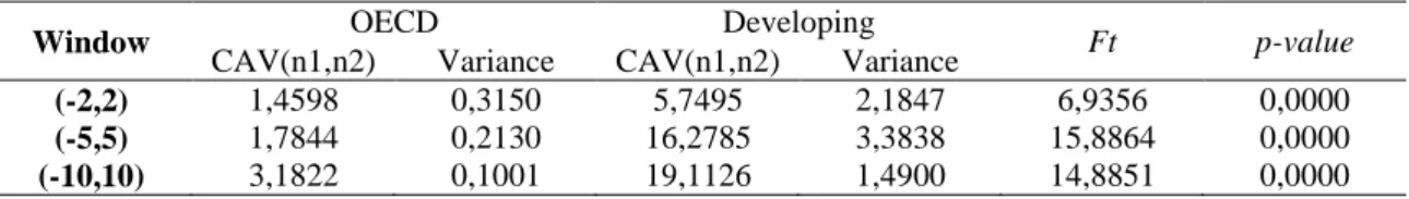
Window OECD Developing Ft p-value

CAV(n1,n2) Variance CAV(n1,n2) Variance

(-2,2) 1,4598 0,3150 5,7495 2,1847 6,9356 0,0000

(-5,5) 1,7844 0,2130 16,2785 3,3838 15,8864 0,0000

(-10,10) 3,1822 0,1001 19,1126 1,4900 14,8851 0,0000

From Table 7 it’s possible to see that there are statistically significant

differences between CAV in Developing and OECD countries in all the windows

considered, allowing us to establish that CAV is higher in Developing countries when

(28)

28 (-25,25), since as seen in Table 6, the CAV values obtained specially in OECD

countries are abnormal.2

Comparing results obtained from 2002-2014 with the results obtained

from 1982-2004

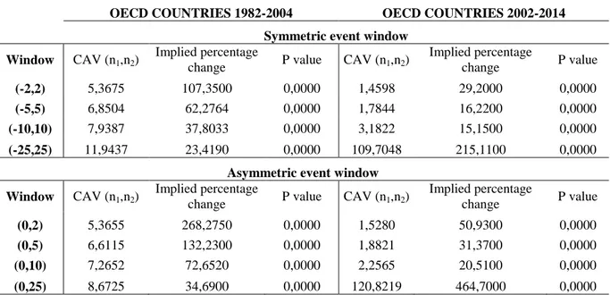
Table 8 - Cumulative abnormal volatility around Election Day on OECD countries: 1982-2004 vs 2002-2014

OECD COUNTRIES 1982-2004 OECD COUNTRIES 2002-2014

Symmetric event window

Implied percentage

change P value

(-2,2) 5,3675 107,3500 0,0000 1,4598 29,2000 0,0000

(-5,5) 6,8504 62,2764 0,0000 1,7844 16,2200 0,0000

(-10,10) 7,9387 37,8033 0,0000 3,1822 15,1500 0,0000

(-25,25) 11,9437 23,4190 0,0000 109,7048 215,1100 0,0000

Asymmetric event window

Implied percentage

change P value

(0,2) 5,3655 268,2750 0,0000 1,5280 50,9300 0,0000

(0,5) 6,6115 132,2300 0,0000 1,8821 31,3700 0,0000

(0,10) 7,2652 72,6520 0,0000 2,2565 20,5100 0,0000

(0,25) 8,6725 34,6900 0,0000 120,8219 464,7000 0,0000

As seen in Table 8, the results of CAV, implied percentage change obtained

between 1982-2004 and 2002-2014 there are some notorious differences. In the period

analyzed in this work (2002-2014), there is still an impact on specific country variance

which is given by the p-value, i. e., independently of the window considered, close to

2

(29)

29 zero. Since the database of the period 1982-2004 was not available, it was not possible

to test the significance of the apparent reported differences.

However, it is important to underline that CAV diminished significantly from

one period to another and the implied percentage change diminished as well. This can

be interpreted as the OECD countries have matured their democracies. Basically, over

the years, the investors started to predict much better the impact of the elections on

monetary and fiscal policy. The investors have the impression that the countries will not

change significantly their monetary and fiscal policy no matters who the Head of the

government is.

Another possible explanation may be that a big part of OECD countries belong

to the Eurozone and because of that the monetary policy does not change from country

to country independently from the elections results.

Determinants of the volatility around Election Day

In order to find further information that links the magnitude of elections shocks

to several explanatory variables a regression analysis was implemented. The dependent

variable was defined as the natural logarithm of the volatility ratio following the

methodology adopted in prior literature (Clayton, Hartzel, & Rosenberg, 2005). This is

the ratio of the return variance computed over the (-25,25) event window by the

variance of the returns in a pre-event of equal length (-76,-26).

As part of the data analysis, the existence of outliers was considered, since they

produce high variability in the analysis, the estimation is affected and the explanation is

reduced. As usual in this type of analysis, the factor considered for identifying an outlier

(30)

30 outputs where initial estimation of the model is made, along with some tests to establish

that the analysis can be made.

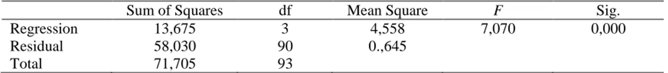
Table 9 - ANOVA for OECD countries after treatment

Sum of Squares df Mean Square F Sig.

Regression 13,675 3 4,558 7,070 0,000

Residual 58,030 90 0.,645

Total 71,705 93

Table 10 - Coefficients for OECD countries after treatment

Unstandardized Coefficients Standardized

Coefficients t Sig. B Std. Error Beta

(Constant) 5,332 1,365 3,907 0,000

Orientation 0,396 0,168 0,227 2,358 0,021

Early -0,401 0,189 -0,203 -2,126 0,036

LN_GDP -0,399 0,130 -0,293 -3,062 0,003

Considering OECD countries, the regression analysis, as seen in Table 9 and

Table 10, shows a statistical significant relation between the dependent variable and a

set of explanatory variables. The F3 test has allowed us to show statistical evidence that

an estimation of a model is possible with a near zero p-value. When analyzing the t test

at a 5% significance level, 3 explanatory variables were identified.

As can be seen in the Table 10, in OECD countries the investors tend to react in

a more volatile manner when there is a change in political orientation as the investors

may anticipate new directions and redistribution policies. The results obtained also tell

that the larger the GDP per capita of a country, the less volatile the market is around

National Elections.

(31)

31 In the previous literature (Bialkowski, Gottschalk, & Wisniewski, 2008) it was

found that the elections called early had a positive impact on stock market volatility.

However, in this sample the result obtained contradicts this result. Finding a reason for

this contradiction is a tough task since it is not intuitive that early elections reduce the

volatility. Probably this happened because of specificities of the sample studied.

The model for OECD countries is expressed by the following equation, with

:

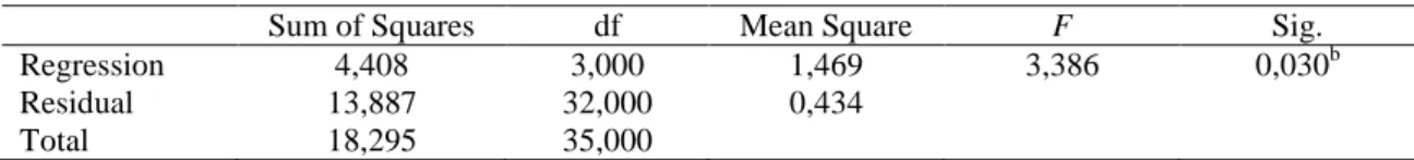
Reasoning as before, we have made the analysis for Developing countries and as

shown in table Table 11 and Table 12. Here again, 3 statistically significant explanatory

variables where identified. For this analysis the 3 variables discussed before

(Democracy, Globalization and Development) were also included. At this point we

make note that the significance of the coefficients estimation is made at a 6,8%

significance level, allowing the variable Age to be included in the model, increasing its

quality.

Table 11 - ANOVA for Developing countries after treatment

Sum of Squares df Mean Square F Sig.

Regression 4,408 3,000 1,469 3,386 0,030b

Residual 13,887 32,000 0,434

Total 18,295 35,000

Table 12 - Coefficients for Developing countries after treatment

Unstandardized Coefficients Standardized

Coefficients t Sig. B Std. Error Beta

(Constant) 0,617 0,395 1,560 0,129

n_Parties 0,294 0,130 0,356 2,269 0,030

Age -0,576 0,306 -0,301 -1,887 0,068

(32)

32 In this case, the number of parties involved in the coalition after the elections

seems to contribute positively for the election shocks. This can happen due to the

perception of the investors that implementing new policies is a hard task when there are

so many parties in the coalition. It is also clear that the stability of a government tends

to be fragile as more parties the government has.

The variable Democracy is measured here as being the average of two indicators

published by The Freedom House: Political rights and Civil Liberties (House, 2015). As

could be expectable, the level of democracy was found as being a variable that is

statistically significant to explain the volatility around the Elections in Developing

countries. Basically, as the coefficient is positive, the lower the democracy level of a

country, in a more volatile manner the markets react.

It is important to note that Political Rights and Civil Liberties published by

Freedom House are two indicators that are being used for “Sustainable Governance

Indicators” and were already launched in 2015. This note reinforces the importance and

credibility of this variable as enriching this project, see (SGI, 2015).

The variable Age appears to be another explanatory variable with significance to

be considered. In this case, it is not easy to find an explanation for the coefficient

obtained as it indicates that in “younger” stock markets is expected lower volatility.

Again, this can be due to some specificities from the sample used.

The model obtained for Developing countries is expressed in the following

equation, with :

(33)

33 It can be argued that since all the stock markets are denominated in US dollars,

the verified volatility can also be due to the movements of foreign exchange markets. In

the paper of (Bialkowski, Gottschalk, & Wisniewski, 2008) it was verified that stock

market volatility is substantially larger than foreign exchange markets even in periods

of closely contested elections which indicates that the contention that the results stem

(34)

34

Conclusions

This study contributes to the analysis of the relationship between finance and

politics by focusing on stock market volatility around national elections.

In this study it is quantified the cumulative abnormal volatility obtained in the

days that surround elections in OECD countries and in Developing countries between

2002 and 2014. This work extends prior results as seen in the literature that just focused

on OECD countries and allows comparing the results with Developing countries.

The first finding that comes from this work is that there is a significant impact in

OECD countries around the national Election Day. The magnitude of this impact was

reduced when compared with the previous results for OECD countries (1982-2004)

volatility but despite lower, the impact is still significant.

In Developing countries, it was found that the investors that operate in these

markets react in a way that the country-specific component of volatility can easily

double so that there is a big fluctuation on stock markets of these countries.

Another important result that arises from this project is that the shock caused by

the elections in the stock market volatility seems to be larger in Developing countries

when compared to OECD countries.

The set of explanatory variables used in this work tried to capture economic,

political, institutional and social factors. In OECD countries, three variables –

Orientation, Early Election and Ln GDP - proved to influence the magnitude of

(35)

35 more volatile way when the outcome of the election reveals a change in political

orientation.

The results shown in this project reinforce prior literature, as seen in

(Bialkowski, Gottschalk, & Wisniewski, 2008), where it was found that a change in

political orientation is a significant variable that explain the results on the volatility.

However, in the update introduced in this project, the formation of minority government

has no longer statistical significance. This can be due to the fact, nowadays, the

politicians are more capable of finding solutions even in minority governments

implying that investors do not see the minority government as a reason to react in a

more volatile manner in the stock market.

Another finding in OECD countries was that smaller the GDP per capita bigger

the impact on stock market volatility.

Regarding Developing countries, the investors see the number of parties of the

coalition as a reason to react. Basically, the investors expect more political problems

with the number of parties in the coalition.

The level of democracy, as defined in this work, is another factor that influences

the investor behavior meaning that they react in a more volatile way when a country is

(36)

36

Future Improvements

From the study developed, some questions arose and might lead to other studies

in the future.

For these future works, in order to consolidate the results obtained, the database

should be increased mainly in Developing countries. This improvement will result in

more robust results. It could be also interesting to compare and understand the

differences between the values of the Cumulative Abnormal Volatility before the

elections and after the elections [(-25,0) vs (0,25)].

The problem detected with abnormal values for CAV in the window (-25,25)

was reported in this study for OECD countries, concerning elections around 2008. It

might be of interest to investigate the reason why such abnormal CAV values were not

reported for Developing countries.

Another possible extension in this work may be to understand the opposite

(37)

37

References

Bank, W. (2015). The World Bank. Retrieved June 2015, from http://data.worldbank.org/ Banks, A. S., Muller, T. C., & Overstreet, W. R. (2004). Political Handbook of the World

2000-2002. Washington DC: CQ Press.

Bialkowski, J., Gottschalk, K., & Wisniewski, T. P. (2008). Stock market volatility around national elections. Journal of Banking and Finance, 1941-1953.

Boehmer, E., Masumeci, J., & Poulsen, A. B. (1991). Event-study methodology under conditions of event-induced variance. Journal of Financial Economics, 253-272.

Clayton, M. J., Hartzel, J. C., & Rosenberg, J. V. (2005). The Impact of CEO Turnover on Equity Volatility. Journal of Business, 1779-1808.

Ejara, D. D., Nag, R., & Upadhyaya, K. P. (2012). Applied Financial Economics. Routledge. EuroStat. (2015). EuroStat. Retrieved from http://ec.europa.eu/eurostat/data/database

Fuss, R., & Bechtel, M. M. (2008). Partisan politics and stock market performance: The effect of expected government partisanship on stock returns in 2002 German federal elections. Public Choice, 131-150.

Goodell, J. W., & Vahamaa, S. (2013). US presidential elections and implied volatility: The role of political uncertainty. Journal of Banking and Finance, 1108-1117.

Grossman, S. J., & Shiller, R. J. (1981). The Determinants of the Variability of Stock Market Prices. ME.

Hilliard, J. E., & Savickas, R. (2002). On the statisctical Significance of Event Effects on Unsystematic Volatility. The Journal of Financial Research, 447-462.

House, F. (2015). Freedom in the World. Retrieved June 25, 2015, from https://freedomhouse.org/report-types/freedom-world#.Vco3FvlVjuo

IDEA. (2015, May 13). International Institute for Democracy and Electoral Assistance. Retrieved June 2015, from http://www.idea.int/vt/compulsory_voting.cfm

KOF. (2015). KOF Index of Globalization. Retrieved June 25, 2015, from http://globalization.kof.ethz.ch/

Macedo, J. B., Pereira, L. B., & Jalles, J. T. (2013). Globalization, Democracy and Development. Cambridge: National Bureau of Economic Research.

Pantzalis, C., Stangeland, D. A., & Turtle, H. J. (2000). Political Elections and the Resolution of Uncertainty: The international Evidence. Journal of Banking and Finance, 1575-1604. Schwert, G. W. (1989). Why Does Stock Market Volatility Change Over Time? The Journal of

(38)

38 SGI. (2015). Sustainable Governance Indicators. Retrieved July 11, 2015, from

http://www.sgi-network.org/2015/

Shiller, R. J. (1981). The Use of Volatility Measures in Assessing Market Efficiency. The Journal of Finance.

(39)

(40)

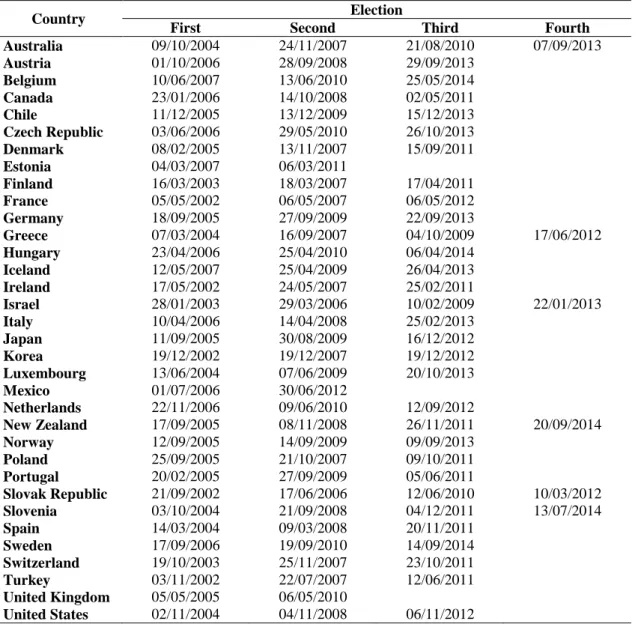
40 Table 13 – Election dates in OECD countries

Country Election

First Second Third Fourth

Australia 09/10/2004 24/11/2007 21/08/2010 07/09/2013

Austria 01/10/2006 28/09/2008 29/09/2013

Belgium 10/06/2007 13/06/2010 25/05/2014

Canada 23/01/2006 14/10/2008 02/05/2011

Chile 11/12/2005 13/12/2009 15/12/2013

Czech Republic 03/06/2006 29/05/2010 26/10/2013

Denmark 08/02/2005 13/11/2007 15/09/2011

Estonia 04/03/2007 06/03/2011

Finland 16/03/2003 18/03/2007 17/04/2011

France 05/05/2002 06/05/2007 06/05/2012

Germany 18/09/2005 27/09/2009 22/09/2013

Greece 07/03/2004 16/09/2007 04/10/2009 17/06/2012

Hungary 23/04/2006 25/04/2010 06/04/2014

Iceland 12/05/2007 25/04/2009 26/04/2013

Ireland 17/05/2002 24/05/2007 25/02/2011

Israel 28/01/2003 29/03/2006 10/02/2009 22/01/2013

Italy 10/04/2006 14/04/2008 25/02/2013

Japan 11/09/2005 30/08/2009 16/12/2012

Korea 19/12/2002 19/12/2007 19/12/2012

Luxembourg 13/06/2004 07/06/2009 20/10/2013

Mexico 01/07/2006 30/06/2012

Netherlands 22/11/2006 09/06/2010 12/09/2012

New Zealand 17/09/2005 08/11/2008 26/11/2011 20/09/2014

Norway 12/09/2005 14/09/2009 09/09/2013

Poland 25/09/2005 21/10/2007 09/10/2011

Portugal 20/02/2005 27/09/2009 05/06/2011

Slovak Republic 21/09/2002 17/06/2006 12/06/2010 10/03/2012

Slovenia 03/10/2004 21/09/2008 04/12/2011 13/07/2014

Spain 14/03/2004 09/03/2008 20/11/2011

Sweden 17/09/2006 19/09/2010 14/09/2014

Switzerland 19/10/2003 25/11/2007 23/10/2011

Turkey 03/11/2002 22/07/2007 12/06/2011

United Kingdom 05/05/2005 06/05/2010

United States 02/11/2004 04/11/2008 06/11/2012

Table 14 – Election dates in Developing countries

Argentina 27/04/2003 28/10/2007 23/10/2011

Brazil 27/10/2002 29/10/2006 31/10/2010

Bulgaria 04/07/2009 11/05/2013

Colombia 26/05/2002 28/05/2006 30/05/2010 25/05/2014

Egypt 07/09/2005 17/06/2012 28/05/2014

India 10/05/2004 13/05/2009 12/05/2014

Indonesia 20/09/2004 08/07/2009 09/07/2014

Malaysia 21/03/2004 08/03/2008 05/05/2013

Pakistan 10/10/2002 18/02/2008 11/05/2013

Philippines 10/05/2004 10/05/2010

Russia 07/12/2003 02/12/2007 04/12/2011

South Africa 14/04/2004 22/04/2009 07/05/2014

(41)

41 Table 15 – Minority Government in OECD countries

Australia 0 0 0 0

Austria 0 0 0

Belgium 0 0 0

Canada 1 1 0

Chile 0 1 0

Czech Republic 0 0 0

Denmark 0 0 0

Estonia 0 0

Finland 0 0 0

France 0 0 0

Germany 0 0 0

Greece 0 0 0 0

Hungary 0 0 0

Iceland 0 0 0

Ireland 0 0 0

Israel 0 0 0 0

Italy 0 0 0

Japan 0 0 0

Korea

Luxembourg 0 0 0

Mexico 0 0

Netherlands 0 0 0

New Zealand 0 0 0 0

Norway 0 0 0

Poland 0 0 0

Portugal 0 1 0

Slovak Republic

Slovenia 0 0 0 0

Spain 1 1 0

Sweden 0 0 1

Switzerland

Turkey 0 0 0

United Kingdom 0 0

United States 0 0 0

Note: 0 – Majority Government; 1 – Minority Government

Table 16 – Minority Government in Developing countries

Argentina 0 0 0

Brazil 0 0 0

Bulgaria 1 0

Colombia 0 0 0 0

Egypt 0 0 0

India 1 1 1

Indonesia 0 0 0

Malaysia 0 0 0

Pakistan 0 0 0

Philippines 0 0

Russia 1 0 0

South Africa 0 0 0

Thailand 0 0

(42)

42 Table 17 – Margin of Victory in OECD countries

Australia -0,0660 -0,1324 -0,1898 -0,0990

Austria 0,3934 0,1048 0,0162

Belgium -0,0216 0,1446 0,0258

Canada -0,2746 -0,2470 -0,2076

Chile 0,0352 -0,1360 -0,0452

Czech Republic -0,0220 -0,0440 -0,1698

Denmark 0,0520 0,1120 0,0040

Estonia 0,1260 0,3240

Finland 0,0760 0,1700 0,2500

France 0,6440 0,0620 0,0320

Germany 0,3884 -0,0328 0,3454

Greece -0,1020 -0,1634 -0,1216 -0,0362

Hungary -0,0300 0,0546 -0,1092

Iceland 0,2680 0,0294 0,0226

Ireland -0,0900 -0,0204 0,1120

Israel 0,3170 0,0506 0,1798 0,0365

Italy -0,0038 -0,0640 -0,4100

Japan -0,0446 -0,0514 -0,1378

Korea

Luxembourg 0,1896 0,1920 -0,0268

Mexico -0,2822 -0,2162

Netherlands 0,0350 -0,0090 0,0284

New Zealand -0,1014 0,0368 -0,0518 -0,0146

Norway -0,0400 -0,0440 0,0780

Poland -0,0720 0,0080 -0,0492

Portugal -0,1000 -0,2680 0,0082

Slovak Republic

Slovenia -0,0194 0,0496 0,0648 0,0130

Spain -0,1482 -0,1220 -0,0900

Sweden -0,0352 -0,0144 -0,2420

Switzerland

Turkey -0,3144 -0,0684 -0,0034

United Kingdom -0,1960 0,1820

United States 0,0240 0,0580 0,0220

Table 18 – Margin of Victory in Developing countries

Argentina -0,0930 0,0820

Brazil 0,2260 0,2166 0,1210

Bulgaria -0,2060 -0,2416

Colombia 0,0800 0,2470 0,3820 0,0190

Egypt 0,7720 0,0356 0,9382

India -0,2920 -0,2556 -0,2200

Indonesia 0,2124 0,2160 0,0630

Malaysia 0,2780 0,0278 -0,0524

Pakistan 0,0944 0,0100 -0,2114

Philippines -0,2002 -0,1984

Russia -0,2486 0,2860 -0,0140

South Africa 0,3938 0,3180 0,2430

(43)

43 Table 19 – Number of Parties in OECD countries

Austria 2 2 2

Belgium 5 6 4

Canada 1 1 1

Chile 1 3 1

Denmark 3 4 4

Estonia 3 3

Finland 3 4 6

France 1 1 1

Germany 2 2 2

Greece 1 1 1 2

Hungary 2 1 1

Iceland 2 2 2

Ireland 2 3 2

Israel 5 4 6 4

Italy 1 1 1

Japan 1 1 1

Korea

Mexico 1 1

Norway 3 3 4

Poland 3 2 2

Portugal 1 2 2

Slovak Republic

Spain 1 1 1

Sweden 4 4 2

Switzerland

Turkey 1 1 1

Table 20 – Number of Parties in Developing countries

Argentina 1 1 1

Brazil 1 1 1

Bulgaria 1 2

Egypt 1 1 1

India 1 1 1

Indonesia 1 1 1

Malaysia 1 1 1

Pakistan 2 2 2

Philippines 1 1

Russia 1 1 1

(44)

44 Table 21 – Change in Orientation in OECD countries

Austria 1 0 0

Belgium 1 1 0

Canada 1 0 0

Chile 0 1 1

Denmark 0 0 0

Estonia 1 0

Finland 1 0 1

France 0 1 1

Germany 1 0 0

Greece 1 0 1 0

Hungary 0 1 0

Iceland 0 1 1

Ireland 0 0 1

Israel 0 1 1 0

Italy 1 1 1

Japan 0 1 1

Korea

Mexico 0 1

Norway 0 0 1

Poland 1 1 0

Portugal 1 0 1

Slovak Republic

Spain 1 0 1

Sweden 1 0 1

Switzerland 1 0 0

Turkey 1 0 0

Note: 0 – No change in orientation; 1 – Change in orientation

Table 22 – Change in Orientation in Developing countries

Argentina 1 0 0

Brazil 1 0 0

Bulgaria 1 1

Egypt 0 1 1

India 1 0 1

Indonesia 1 0 1

Malaysia 0 0 0

Pakistan 1 1 1

Philippines 1 1

Russia 1 0 0

Thailand 0 0

(45)

45 Table 23 – Early Election in OECD countries

Austria 0 1 0

Belgium 0 1 0

Canada 1 1 1

Chile 0 0 0

Denmark 0 1 0

Estonia 0 0

Finland 0 0 0

France 0 0 0

Germany 0 0 0

Greece 0 1 1 1

Hungary 0 0 0

Iceland 0 1 0

Ireland 0 1 0

Israel 1 1 1 1

Italy 0 1 0

Japan 1 0 1

Korea

Mexico 0 0

Norway 0 0 0

Poland 0 1 0

Portugal 1 0 1

Slovak Republic

Spain 0 0 1

Sweden 0 0 0

Switzerland 0 0 0

Turkey 0 0 0

Note: 0 – No early election; 1 – Early election

Table 24 – Early Election in Developing countries

Argentina 0 0 0

Brazil 0 0 0

Bulgaria 0 1

Egypt 0 0 1

India 0 0 0

Indonesia 0 0 0

Malaysia 0 0 1

Pakistan 0 0 0

Philippines 0 0

Russia 0 0 0

Thailand 1 0

Elections and stock market volatility: evidence in OECD countries and developing countries

Acknowledgements

Resumo

Abstract

Contents

List of Tables

Introduction

Literature Review

Methodology

Data

Results

Comparing results obtained from 2002-2014 with the results obtained

from 1982-2004

Determinants of the volatility around Election Day

Conclusions

Future Improvements

References