The Mathematics of Infectious
Diseases
∗
Herbert W. Hethcote†
Abstract.Many models for the spread of infectious diseases in populations have been analyzed math-ematically and applied to specific diseases. Threshold theorems involving the basic repro-duction numberR0, the contact numberσ, and the replacement numberRare reviewed for the classic SIR epidemic and endemic models. Similar results with new expressions for
R0 are obtained for MSEIR and SEIR endemic models with either continuous age or age
groups. Values ofR0 andσare estimated for various diseases including measles in Niger and pertussis in the United States. Previous models with age structure, heterogeneity, and spatial structure are surveyed.
Key words.thresholds, basic reproduction number, contact number, epidemiology, infectious diseases
AMS subject classifications.Primary, 92D30; Secondary, 34C23, 34C60, 35B32, 35F25
PII.S0036144500371907
1. Introduction. The effectiveness of improved sanitation, antibiotics, and vac-cination programs created a confidence in the 1960s that infectious diseases would soon be eliminated. Consequently, chronic diseases such as cardiovascular disease and cancer received more attention in the United States and industrialized countries. But infectious diseases have continued to be the major causes of suffering and mortality in developing countries. Moreover, infectious disease agents adapt and evolve, so that new infectious diseases have emerged and some existing diseases have reemerged [142]. Newly identified diseases include Lyme disease (1975), Legionnaire’s disease (1976), toxic-shock syndrome (1978), hepatitis C (1989), hepatitis E (1990), and hantavirus (1993). The human immunodeficiency virus (HIV), which is the etiological agent for acquired immunodeficiency syndrome (AIDS), emerged in 1981 and has become an important sexually transmitted disease throughout the world. Antibiotic-resistant strains of tuberculosis, pneumonia, and gonorrhea have evolved. Malaria, dengue, and yellow fever have reemerged and are spreading into new regions as climate changes occur. Diseases such as plague, cholera, and hemorrhagic fevers (Bolivian, Ebola, Lassa, Marburg, etc.) continue to erupt occasionally. Surprisingly, new infectious agents called prions have recently joined the previously known agents: viruses, bac-teria, protozoa, and helminths (worms). There is strong evidence that prions are the cause of spongiform encephalopathies, e.g., bovine spongiform encephalopathy (BSE, “mad cow disease”), Creutzfeldt-Jakob disease (CJD), kuru, and scrapie in sheep [168]. Recent popular books have given us exciting accounts of the emergence and de-tection of new diseases [82, 168, 170, 183]. It is clear that human or animal invasions
∗Received by the editors March 6, 2000; accepted for publication (in revised form) May 7, 2000;
published electronically October 30, 2000.
http://www.siam.org/journals/sirev/42-4/37190.html
†Department of Mathematics, University of Iowa, Iowa City, IA 52242 (hethcote@math.
uiowa.edu).
of new ecosystems, global warming, environmental degradation, increased interna-tional travel, and changes in economic patterns will continue to provide opportunities for new and existing infectious diseases [152].
The emerging and reemerging diseases have led to a revived interest in infec-tious diseases. Mathematical models have become important tools in analyzing the spread and control of infectious diseases. The model formulation process clarifies as-sumptions, variables, and parameters; moreover, models provide conceptual results such as thresholds, basic reproduction numbers, contact numbers, and replacement numbers. Mathematical models and computer simulations are useful experimental tools for building and testing theories, assessing quantitative conjectures, answer-ing specific questions, determinanswer-ing sensitivities to changes in parameter values, and estimating key parameters from data. Understanding the transmission characteris-tics of infectious diseases in communities, regions, and countries can lead to better approaches to decreasing the transmission of these diseases. Mathematical models are used in comparing, planning, implementing, evaluating, and optimizing various detection, prevention, therapy, and control programs. Epidemiology modeling can contribute to the design and analysis of epidemiological surveys, suggest crucial data that should be collected, identify trends, make general forecasts, and estimate the uncertainty in forecasts [100, 111].
Although a model for smallpox was formulated and solved by Daniel Bernoulli in 1760 in order to evaluate the effectiveness of variolation of healthy people with the smallpox virus [24], deterministic epidemiology modeling seems to have started in the 20th century. In 1906 Hamer formulated and analyzed a discrete time model in his attempt to understand the recurrence of measles epidemics [95]. His model may have been the first to assume that the incidence (number of new cases per unit time) depends on the product of the densities of the susceptibles and infectives. Ross was interested in the incidence and control of malaria, so he developed differential equation models for malaria as a host-vector disease in 1911 [173]. Other determin-istic epidemiology models were then developed in papers by Ross, Ross and Hudson, Martini, and Lotka [18, 60, 66]. Starting in 1926 Kermack and McKendrick published papers on epidemic models and obtained the epidemic threshold result that the den-sity of susceptibles must exceed a critical value in order for an epidemic outbreak to occur [18, 136, 157]. Mathematical epidemiology seems to have grown exponentially starting in the middle of the 20th century (the first edition in 1957 of Bailey’s book [18] is an important landmark), so that a tremendous variety of models have now been formulated, mathematically analyzed, and applied to infectious diseases. Re-views of the literature [21, 39, 60, 65, 67, 102, 107, 109, 199] show the rapid growth of epidemiology modeling. The recent models have involved aspects such as passive immunity, gradual loss of vaccine and disease-acquired immunity, stages of infection, vertical transmission, disease vectors, macroparasitic loads, age structure, social and sexual mixing groups, spatial spread, vaccination, quarantine, and chemotherapy. Special models have been formulated for diseases such as measles, rubella, chicken-pox, whooping cough, diphtheria, smallchicken-pox, malaria, onchocerciasis, filariasis, rabies, gonorrhea, herpes, syphilis, and HIV/AIDS. The breadth of the subject is shown in the books on epidemiology modeling [5, 9, 12, 18, 19, 20, 22, 33, 38, 39, 55, 56, 59, 80, 81, 90, 111, 113, 127, 137, 141, 151, 164, 167, 173, 181, 194, 196].
M
❄ births with passive immunity✲ transf er f rom M
❄ deaths
S
❄births without passive immunity
✲ horizontal
incidence
❄ deaths
E
transf er✲ f rom E❄ deaths
I
transf er✲ f rom I❄ deaths
R
❄ deaths
Fig. 1 The general transfer diagram for the MSEIR model with the passively immune class M, the susceptible class S, the exposed class E, the infective class I, and the recovered class R.
temporary passive immunity to an infection. The class M contains these infants with passive immunity. After the maternal antibodies disappear from the body, the in-fant moves to the susceptible class S. Inin-fants who do not have any passive immunity, because their mothers were never infected, also enter the class S of susceptible indi-viduals; that is, those who can become infected. When there is an adequate contact of a susceptible with an infective so that transmission occurs, then the susceptible enters the exposed class E of those in the latent period, who are infected but not yet infectious. After the latent period ends, the individual enters the class I of infectives, who are infectious in the sense that they are capable of transmitting the infection. When the infectious period ends, the individual enters the recovered class R consisting of those with permanent infection-acquired immunity.
The choice of which compartments to include in a model depends on the charac-teristics of the particular disease being modeled and the purpose of the model. The passively immune class M and the latent period class E are often omitted, because they are not crucial for the susceptible-infective interaction. Acronyms for epidemi-ology models are often based on the flow patterns between the compartments such as MSEIR, MSEIRS, SEIR, SEIRS, SIR, SIRS, SEI, SEIS, SI, and SIS. For example, in the MSEIR model shown in Figure 1, passively immune newborns first become sus-ceptible, then exposed in the latent period, then infectious, and then removed with permanent immunity. An MSEIRS model would be similar, but the immunity in the R class would be temporary, so that individuals would regain their susceptibility when the temporary immunity ended.
The threshold for many epidemiology models is the basic reproduction number R0, which is defined as the average number of secondary infections produced when one infected individual is introduced into a host population where everyone is suscep-tible [61]. For many deterministic epidemiology models, an infection can get started in a fully susceptible population if and only if R0 > 1. Thus the basic reproduc-tion numberR0 is often considered as the threshold quantity that determines when an infection can invade and persist in a new host population. Section 2 introduces epidemiology modeling by formulating and analyzing two classic deterministic mod-els. The role ofR0is demonstrated for the classic SIR endemic model in section 2.4. Then thresholds are estimated from data on several diseases and the implications of the estimates are considered for diseases such as smallpox, polio, measles, rubella, chickenpox, and influenza. An MSEIR endemic model in a population without age structure but with exponentially changing population size is formulated and analyzed in section 3. This model demonstrates how exponential population growth affects the basic reproduction numberR0.
pro-grams often focus on specific ages, and epidemiologic data is often age specific. These epidemiologic models are based on the demographic models in section 4 with either continuous age or age groups. The two demographic models demonstrate the role of the population reproduction numbers in determining when the population grows asymptotically exponentially. The MSEIR with continuous age structure is formu-lated and analyzed in section 5. New general expressions for the basic reproduction number R0 and the average age of infection A are obtained. Expressions for these quantities are found in sections 5.4 and 5.6 in the cases when the survival function of the population is a negative exponential and a step function. In section 5.5 the en-demic threshold and the average age of infection are obtained when vaccination occurs at ageAv. The SEIR model with age groups is formulated and analyzed in section 6.
The new expressions for the basic reproduction number R0 and the average age of infection A are analogous to those obtained for the MSEIR model with continuous age structure.
The theoretical expressions in section 6 are used in section 7 to obtain estimates of the basic reproduction numberR0 and the average age of infectionA for measles in Niger, Africa. These estimates are affected by the very rapid 3.3% growth of the population in Niger. In section 8 estimates of the basic reproduction numberR0and the contact number σ (defined in section 2.2) are obtained for pertussis (whooping cough) in the United States. Because pertussis infectives with lower infectivity occur in previously infected people, the contact number σ at the endemic steady state is less than the basic reproduction numberR0. Section 9 describes results on the basic reproduction numberR0for previous epidemiology models with a variety of structures, and section 10 contains a general discussion.
2. Two Classic Epidemiology Models. In order to introduce the terminology, notation, and standard results for epidemiology models, two classic SIR models are formulated and analyzed. Epidemic models are used to describe rapid outbreaks that occur in less than one year, while endemic models are used for studying diseases over longer periods, during which there is a renewal of susceptibles by births or recovery from temporary immunity. The two classic SIR models provide an intuitive basis for understanding more complex epidemiology modeling results.
2.1. FormulatingEpidemiology Models. The horizontal incidence shown in Fig-ure 1 is the infection rate of susceptible individuals through their contacts with infec-tives. IfS(t) is the number of susceptibles at timet, I(t) is the number of infectives, and N is the total population size, then s(t) = S(t)/N and i(t) = I(t)/N are the susceptible and infectious fractions, respectively. If β is the average number of ad-equate contacts (i.e., contacts sufficient for transmission) of a person per unit time, thenβI/N =βiis the average number of contacts with infectives per unit time of one susceptible, and (βI/N)S =βN is is the number of new cases per unit time due to theS =N ssusceptibles. This form of the horizontal incidence is called the standard incidence, because it is formulated from the basic principles above [96, 102].
on the population size. Using an incidence of the formηNvSI/N, data for five human
diseases in communities with population sizes from 1,000 to 400,000 [9, p. 157] [12, p. 306] imply thatvis between 0.03 and 0.07. This strongly suggests that the standard incidence corresponding tov= 0 is more realistic for human diseases than the simple mass action incidence corresponding to v = 1. This result is consistent with the concept that people are infected through their daily encounters and the patterns of daily encounters are largely independent of community size within a given country (e.g., students of the same age in a country usually have a similar number of daily contacts).
The standard incidence is also a better formulation than the simple mass action law for animal populations such as mice in a mouse-room or animals in a herd [57], because disease transmission primarily occurs locally from nearby animals. For more information about the differences in models using these two forms of the horizontal incidence, see [83, 84, 85, 96, 110, 159]. Vertical incidence, which is the infection rate of newborns by their mothers, is sometimes included in epidemiology models by assuming that a fixed fraction of the newborns is infected vertically [33]. Models with population size–dependent contact functions have also been considered [29, 171, 190, 191, 201]. Various forms of nonlinear incidences have been considered [112, 147, 148, 149]. See [107] for a survey of mechanisms including nonlinear incidences that can lead to periodicity in epidemiological models.
A common assumption is that the movements out of the M, E, and I compart-ments and into the next compartment are governed by terms likeδM,ǫE, andγI in an ordinary differential equations model. It has been shown [109] that these terms correspond to exponentially distributed waiting times in the compartments. For ex-ample, the transfer rate γI corresponds to P(t) = e−γt as the fraction that is still
in the infective class t units after entering this class and to 1/γ as the mean wait-ing time. For measles the mean period 1/δ of passive immunity is about six to nine months, while the mean latent period 1/ε is one to two weeks and the mean infec-tious period 1/γ is about one week. Another possible assumption is that the fraction still in the compartment t units after entering is a nonincreasing, piecewise contin-uous function P(t) with P(0) = 1 and P(∞) = 0. Then the rate of leaving the compartment at time t is −P′(t), so the mean waiting time in the compartment is
∞
0 t(−P
′(t))dt=∞
0 P(t)dt. These distributed delays lead to epidemiology models with integral or integrodifferential or functional differential equations. If the waiting time distribution is a step function given by P(t) = 1 if 0 ≤ t ≤τ, andP(t) = 0 if τ ≤ t, then the mean waiting time is τ, and for t ≥ τ the model reduces to a delay-differential equation [109]. Each waiting time in a model can have a different distribution, so there are many possible models [102].
Table 1 Summary of notation.
M Passively immune infants
S Susceptibles
E Exposed people in the latent period
I Infectives
R Recovered people with immunity
m, s, e, i, r Fractions of the population in the classes above
β Contact rate
1/δ Average period of passive immunity 1/ε Average latent period
1/γ Average infectious period
R0 Basic reproduction number
σ Contact number
R Replacement number
typical infective during the entire period of infectiousness [96]. Some authors use the term reproduction number instead of replacement number, but it is better to avoid the name reproduction number since it is easily confused with the basic reproduction number. Note that these three quantitiesR0,σ, andRin Table 1 are all equal at the beginning of the spread of an infectious disease when the entire population (except the infective invader) is susceptible. In recent epidemiological modeling literature, the basic reproduction numberR0is often used as the threshold quantity that determines whether a disease can invade a population.
Although R0 is only defined at the time of invasion, σ and R are defined at all times. For most models, the contact number σ remains constant as the infection spreads, so it is always equal to the basic reproduction numberR0. In these models σandR0can be used interchangeably and invasion theorems can be stated in terms of either quantity. But for the pertussis models in section 8, the contact numberσ becomes less than the basic reproduction numberR0after the invasion, because new classes of infectives with lower infectivity appear when the disease has entered the population. The replacement numberRis the actual number of secondary cases from a typical infective, so that after the infection has invaded a population and everyone is no longer susceptible,Ris always less than the basic reproduction numberR0. Also, after the invasion, the susceptible fraction is less than 1, so that not all adequate contacts result in a new case. Thus the replacement numberRis always less than the contact numberσafter the invasion. Combining these results leads to
R0≥σ≥R,
with equality of the three quantities at the time of invasion. Note that R0 =σ for most models, andσ > R after the invasion for all models.
2.3. The Classic Epidemic Model. Using the notation in section 2.1, the classic epidemic model is the SIR model given by the initial value problem
dS/dt=−βIS/N, S(0) =So≥0,
dI/dt=βIS/N−γI, I(0) =Io≥0,
dR/dt=γI, R(0) =Ro≥0,
(2.1)
0 0.2 0.4 0.6 0.8 1
susceptible fraction, s
0 0.2 0.4 0.6 0.8 1
infective
fraction,
i
smax
↑
=1
σ
σ= 3
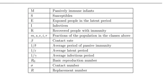
Fig. 2 Phase plane portrait for the classic SIR epidemic model with contact numberσ= 3.
passively immune class M and the exposed class E are omitted. This model uses the standard incidence and has recovery at rateγI, corresponding to an exponential waiting time e−γt. Since the time period is short, this model has no vital dynamics
(births and deaths). Dividing the equations in (2.1) by the constant total population sizeN yields
ds/dt=−βis, s(0) =so≥0,
di/dt=βis−γi, i(0) =io≥0,
(2.2)
withr(t) = 1−s(t)−i(t), wheres(t), i(t), andr(t) are the fractions in the classes. The triangleT in the siphase plane given by
T ={(s, i)|s≥0, i≥0, s+i≤1}
(2.3)
0 5 10 15 20 25
time in days
0 0.2 0.4 0.6 0.8 1
infective fraction susceptible fraction
σ= 3
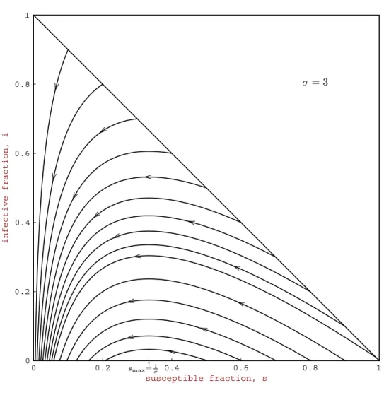
Fig. 3 Solutions of the classic SIR epidemic model with contact numberσ= 3and average infectious period1/γ= 3days.
Fig. 4 Reported number of measles cases in the Netherlands by week of onset and vaccination status
during April1999 to January2000. Most of the unvaccinated cases were people belonging
contacts of a typical infective during the infectious period. Here the replacement number at time zero is σso, which is the product of the contact number σ and the
initial susceptible fractionso.
Theorem 2.1. Let (s(t), i(t))be a solution of (2.2)in T. If σso ≤1, then i(t)
decreases to zero as t → ∞. If σso >1, then i(t) first increases up to a maximum
value imax = io+so−1/σ −[ln(σso)]/σ and then decreases to zero as t → ∞.
The susceptible fractions(t)is a decreasing function and the limiting values∞ is the
unique root in (0,1/σ)of the equation
io+so−s∞+ ln(s∞/so)/σ= 0.
(2.4)
Typical paths in T are shown in Figure 2, and solutions as a function of time are shown in Figure 3. Note that the hallmark of a typical epidemic outbreak is an infective curve that first increases from an initialIonear zero, reaches a peak, and then
decreases toward zero as a function of time. For example, a recent measles epidemic in the Netherlands [52] is shown in Figure 4. The susceptible fraction s(t) always decreases, but the final susceptible fraction s∞ is positive. The epidemic dies out because, when the susceptible fractions(t) goes below 1/σ, the replacement number σs(t) goes below 1. The results in the theorem are epidemiologically reasonable, since the infectives decrease and there is no epidemic, if enough people are already immune so that a typical infective initially replaces itself with no more than one new infective (σso ≤1). But if a typical infective initially replaces itself with more than one new
infective (σso>1), then infectives initially increase so that an epidemic occurs. The
speed at which an epidemic progresses depends on the characteristics of the disease. The measles epidemic in Figure 4 lasted for about nine months, but because the latent period for influenza is only one to three days and the infectious period is only two to three days, an influenza epidemic can sweep through a city in less than six weeks. See [100] for more examples of epidemic outbreak curves.
To prove the theorem, observe that the solution paths
i(t) +s(t)−[lns(t)]/σ=io+so−[lnso]/σ
in Figure 2 are found from the quotient differential equation di/ds =−1 + 1/(σs). The equilibrium points along the s axis are neutrally unstable for s > 1/σ and are neutrally stable for s < 1/σ. For a complete (easy) proof, see [96] or [100]. One classic approximation derived in [18] is that for smallio andso slightly greater than
smax = 1/σ, the difference smax−s(∞) is about equal to so−smax, so the final
susceptible fraction is about as far below the susceptible fraction smax (the s value where the infective fraction is a maximum) as the initial susceptible fraction was above it (see Figure 2). Observe that the threshold result here involves the initial replacement numberσso and does not involve the basic reproduction numberR0.
2.4. The Classic Endemic Model. The classic endemic model is the SIR model with vital dynamics (births and deaths) given by
dS/dt=µN−µS−βIS/N, S(0) =So≥0,
dI/dt=βIS/N−γI−µI, I(0) =Io≥0,
dR/dt=γI−µR, R(0) =Ro≥0,
(2.5)
at rateµN and deaths in the classes at rates µS, µI, and µR. The deaths balance the births, so that the population sizeNis constant. The mean lifetime 1/µwould be about 75 years in the United States. Dividing the equations in (2.5) by the constant total population sizeN yields
ds/dt=−βis+µ−µs, s(0) =so≥0,
di/dt=βis−(γ+µ)i, i(0) =io≥0,
(2.6)
with r(t) = 1−s(t)−i(t). The triangle T in the si phase plane given by (2.3) is positively invariant, and the model is well posed [96]. Here the contact numberσ remains equal to the basic reproduction numberR0for all time, because no new classes of susceptibles or infectives occur after the invasion. For this model the threshold quantity is given by R0 = σ = β/(γ +µ), which is the contact rate β times the average death-adjusted infectious period 1/(γ+µ).
Theorem 2.2. Let(s(t), i(t))be a solution of(2.6)inT. Ifσ≤1orio= 0, then
solution paths starting inT approach the disease-free equilibrium given bys= 1and
i= 0. Ifσ >1, then all solution paths with io>0 approach the endemic equilibrium
given byse= 1/σ andie=µ(σ−1)/β.
Figures 5 and 6 illustrate the two possibilities given in the theorem. IfR0=σ≤1, then the replacement number σs is less than 1 when io > 0, so that the
infec-tives decrease to zero. Although the speeds of movement along the paths are not apparent from Figure 5, the infective fraction decreases rapidly to very near zero, and then over 100 or more years, the recovered people slowly die off and the birth process slowly increases the susceptibles, until eventually everyone is susceptible at the disease-free equilibrium with s = 1 and i = 0. If R0 = σ > 1, io is small,
and so is large with σso > 1, then s(t) decreases and i(t) increases up to a peak
and then decreases, just as it would for an epidemic (compare Figure 6 with Fig-ure 2). However, after the infective fraction has decreased to a low level, the slow processes of the deaths of recovered people and the births of new susceptibles grad-ually (over about 10 or 20 years) increase the susceptible fraction untilσs(t) is large enough that another smaller epidemic occurs. This process of alternating rapid epi-demics and slow regeneration of susceptibles continues as the paths approach the en-demic equilibrium given in the theorem. At this enen-demic equilibrium the replacement number σse is 1, which is plausible since if the replacement number were greater
than or less than 1, the infective fraction i(t) would be increasing or decreasing, respectively.
Theorem 2.2 was proved in [96] and in [100] using phase plane methods and Liapunov functions. For this SIR model there is a transcritical (stability exchange) bifurcation at σ = 1, as shown in Figure 7. Notice that the ie coordinate of the
endemic equilibrium is negative forσ <1, coincides with the disease-free equilibrium value of zero at σ = 1, and becomes positive forσ > 1. This equilibrium given by se = 1/σ and ie = µ(σ−1)/β is unstable for σ < 1 and is locally asymptotically
0 0.2 0.4 0.6 0.8 1
susceptible fraction, s
0 0.2 0.4 0.6 0.8 1
infective
fraction,
i
R0=σ= 0.5
Fig. 5 Phase plane portrait for the classic SIR endemic model with contact numberσ= 0.5.
SEIR model the global stability below the threshold was proved in [147] and the global stability above the threshold was recently proved using clever new methods [143]. Results for the MSEIR model are given in section 3.
The following interpretation of the results in the theorem and paragraph above is one reason why the basic reproduction numberR0 has become widely used in the epidemiology literature. If the basic reproduction numberR0(which is always equal to the contact numberσwhen the entire population is susceptible) is less than 1, then the disease-free equilibrium is locally asymptotically stable and the disease cannot “invade” the population. But ifR0>1, then the disease-free equilibrium is unstable with a repulsive direction into the positive siquadrant, so the disease can “invade” in the sense that any path starting with a small positiveio moves into the positivesi
0 0.2 0.4 0.6 0.8 1
susceptible fraction, s
0 0.2 0.4 0.6 0.8 1
infective
fraction,
i
1/σ
R0=σ= 3
Fig. 6 Phase plane portrait for the classic SIR endemic model with contact numberσ= 3, average infectious period1/γ = 3 days, and average lifetime1/µ= 60 days. This unrealistically short average lifetime has been chosen so that the endemic equilibrium is clearly above the horizontal axis and the spiraling into the endemic equilibrium can be seen.
2.5. Threshold Estimates Usingthe Classic Models. The classic SIR models above are very important as conceptual models (similar to predator-prey and compet-ing species models in ecology). The SIR epidemic modelcompet-ing yields the useful concept of the threshold quantityσso, which determines when an epidemic occurs, and formulas
for the peak infective fraction im and the final susceptible fraction s∞. The SIR endemic modeling yields R0 = σ as the threshold quantity that determines when the disease remains endemic, the concept that the infective replacement numberσse
is 1 at the endemic equilibrium, and the explicit dependence of the infective frac-tion ie on the parameters. However, these simple, classic SIR models have obvious
0 0.5 1 1.5 2 2.5 3 −0.3
−0.2 −0.1 0 0.1 0.2 0.3 0.4 0.5 0.6
BIFURCATION DIAGRAM FOR THE SIR ENDEMIC MODEL
infective fraction, i
stable disease− free equilibrium
unstable disease−free equilibrium
unstable endemic equilibrium
stable endemic equilibrium
contact number,σ
Fig. 7 The bifurcation diagram for the SIR endemic model, which shows that the disease-free and endemic equilibria exchange stability when the contact numberσis1.
From (2.4) fors∞in the classic SIR epidemic model, the approximation
σ≈ ln(so/s∞)
so−s∞
follows because io is negligibly small. By using data on the susceptible fractions so
ands∞ at the beginning and end of epidemics, this formula can be used to estimate contact numbers for specific diseases [100]. Using blood samples from freshmen at Yale University [75], the fractions susceptible to rubella at the beginning and end of the freshman year were found to be 0.25 and 0.090, so the epidemic formula above gives σ≈6.4. The fractionsso= 0.49 ands∞= 0.425 for the Epstein–Barr virus (related to mononucleosis) lead to σ≈2.2, and the fractions so= 0.911 and s∞= 0.514 for influenza (H3N2 type A “Hong Kong”) lead toσ≈1.44. For the 1957 “Asian Flu” (H2N2 type A strain of influenza) in Melbourne, Australia, the fractionsso= 1 and
s∞ = 0.55 from [31, p. 129] yield the contact number estimate σ≈1.33. Thus the easy theory for the classic SIR epidemic model yields the formula above that can be used to estimate contact numbers from epidemic data.
fraction of the samples that are not seropositive, sincese= 1−ie−re. This approach
is somewhat naive, because the average seropositivity in a population decreases to zero as the initial passive immunity declines and then increases as people age and are exposed to infectives. Thus the ages of those sampled are critical in using the estimate σ= 1/se. For the SIR model with negative exponential survival in section 5.4, one
estimation formula for the basic reproduction number isR0= 1 +L/A, whereLis the average lifetime 1/µ and A is the average age of infection. This estimation formula can also be derived heuristically from the classic SIR endemic model. The incidence rate at the endemic equilibrium is βiese, so thatβie is the incidence rate constant,
which with exponential waiting time implies that the average age of infection (the mean waiting time in S) is A= 1/βie= 1/[µ(σ−1)]. Using µ= 1/L, this leads to
R0=σ= 1 +L/A, sinceR0=σ for this model.
Data on average ages of infection and average lifetimes in developed countries have been used to estimate basic reproduction numbers R0 for some viral diseases. These estimates ofR0 are about 16 for measles, 11 for varicella (chickenpox), 12 for mumps, 7 for rubella, and 5 for poliomyelitis and smallpox [12, p. 70], [100]. Because disease-acquired immunity is only temporary for bacterial diseases such as pertussis (whooping cough) and diphtheria, the formulaR0 =σ= 1 +L/Acannot be used to estimateR0 for these diseases (see section 8 for estimates ofR0and σfor pertussis). Herd immunity occurs for a disease if enough people have disease-acquired or vaccination-acquired immunity, so that the introduction of one infective into the pop-ulation does not cause an invasion of the disease. Intuitively, if the contact number is σ, so that the typical infective has adequate contacts with σ people during the infectious period, then the replacement number σs must be less than 1 so that the disease does not spread. This means that s must be less than 1/σ, so the immune fraction rmust satisfy r >1−1/σ = 1−1/R0. For example, if R0 =σ= 10, then the immune fraction must satisfyr >1−1/10 = 0.9, so that the replacement number is less than 1 and the disease does not invade the population.
Using the estimates above for R0, the minimum immune fractions for herd im-munity are 0.94 for measles, 0.89 for mumps, 0.86 for rubella, and 0.8 for poliomyeli-tis and smallpox. Although these values give only crude, ballpark estimates for the vaccination-acquired immunity level in a community required for herd immunity, they are useful for comparing diseases. For example, these numbers suggest that it should be easier to achieve herd immunity for poliomyelitis and smallpox than for measles, mumps, and rubella. This conclusion is justified by the actual effectiveness of vaccina-tion programs in reducing, locally eliminating, and eradicating these diseases (eradi-cation means elimination throughout the world). The information in the next section verifies that smallpox has been eradicated worldwide and polio should be eradicated worldwide within a few years, while the diseases of rubella and measles still persist at low levels in the United States and at higher levels in many other countries. Thus the next section provides historical context and verifies the disease comparisons obtained from the simple, classic SIR endemic model.
This was the world’s first vaccine (vacca is the Latin word for cow). Two years later, the findings of the first vaccine trials were published, and by the early 1800s, the smallpox vaccine was widely available. Smallpox vaccination was used in many countries in the 19th century, but smallpox remained endemic. When the World Health Organization (WHO) started a global smallpox eradication program in 1967, there were about 15 million cases per year, of which 2 million died and millions more were disfigured or blinded by the disease [77]. The WHO strategy involved extensive vaccination programs (see Figure 8), surveillance for smallpox outbreaks, and containment of these outbreaks by local vaccination programs. There are some interesting stories about the WHO campaign, including the persuasion of African chiefs to allow their tribes to be vaccinated and monetary bounty systems for finding hidden smallpox cases in India. Smallpox was slowly eliminated from many countries, with the last case in the Americas in 1971. The last case worldwide was in Somalia in 1977, so smallpox has been eradicated throughout the world [23, 77, 168]. The WHO estimates that the elimination of worldwide smallpox vaccination saves over two billion dollars per year. The smallpox virus has been kept in U.S. and Russian government laboratories; the United States keeps it so that vaccine could be produced if smallpox were ever used in biological terrorism [182].
Most cases of poliomyelitis are asymptomatic, but a small fraction of cases result in paralysis. In the 1950s in the United States, there were about 60,000 paralytic polio cases per year. In 1955 Jonas Salk developed an injectable polio vaccine from an inactivated polio virus. This vaccine provides protection for the person, but the person can still harbor live viruses in their intestines and can pass them to others. In 1961 Albert Sabin developed an oral polio vaccine from weakened strains of the polio virus. This vaccine provokes a powerful immune response, so the person cannot harbor the “wild-type” polio viruses, but a very small fraction (about one in 2 million) of those receiving the oral vaccine develop paralytic polio [23, 168]. The Salk vaccine interrupted polio transmission and the Sabin vaccine eliminated polio epidemics in the United States, so there have been no indigenous cases of naturally occurring polio since 1979. In order to eliminate the few cases of vaccine-related paralytic polio each year, the United States now recommends the Salk injectable vaccine for the first four polio vaccinations, even though it is more expensive [50]. In the Americas, the last case of paralytic polio caused by the wild virus was in Peru in 1991. In 1988 the WHO set a goal of global polio eradication by the year 2000 [178]. Most countries are using the live-attenuated Sabin vaccine, because it is inexpensive (8 cents per dose) and can be easily administered into a mouth by an untrained volunteer. The WHO strategy includes routine vaccination, National Immunization Days (during which many people in a country or region are vaccinated in order to interrupt transmission), mopping-up vaccinations, and surveillance for acute flaccid paralysis [116]. Polio has disappeared from many countries in the past 10 years, so that by 1999 it was concentrated in the Eastern Mediterranean region, South Asia, West Africa, and Central Africa. It is likely that polio will soon be eradicated worldwide. The WHO estimates that eradicating polio will save about $1.5 billion each year in immunization, treatment, and rehabilitation around the globe [45].
Fig. 8 Following Jenner’s discovery in 1796, smallpox vaccination spread throughout the world
within decades. But the replacement numberR remained above 1, so that smallpox
per-sisted in most areas until the mid-20th century. In1966smallpox was still endemic in South America, Africa, India, and Indonesia. After the WHO smallpox eradication program was initiated in 1967, the worldwide incidence of the disease decreased steadily. Posters like these motivated people in Africa to get smallpox vaccinations. The last naturally occurring
smallpox case was in Somalia in1977. Reprinted from Centers for Disease Control HHS
Publication No. (CDC)87-8400.
Fig. 9 After a measles vaccine was approved in1963,vaccination programs in the United States were very effective in reducing reported measles cases. This1976photograph shows schoolchildren in Highland Park, Illinois, lining up for measles vaccinations. Because of a major outbreak in1989–1991, the United States changed to a two-dose measles vaccination program. The
replacement number R now appears to be below 1 throughout the United States, so that
measles is no longer considered to be an indigenous disease there. Photo by Thomas S. England, Photo Researchers, Inc.
than 0.94 for measles and 0.86 for rubella. But the vaccine efficacy for these diseases is about 0.95, which means that 5% of those who are vaccinated do not become immune. Thus to reach the levels necessary to achieve herd immunity, the vaccinated fractions would have to be at least 0.99 for measles and 0.91 for rubella. These fractions suggest that achieving herd immunity would be much harder for measles than for rubella, because the percentages not vaccinated would have to be below 1% for measles and below 9% for rubella. Because vaccinating all but 1% against measles would be difficult to achieve, a two-dose program for measles is an attractive alternative in some countries [50, 98, 99].
replaced with a two-dose program with the first measles vaccination at age 12 to 15 months and the second vaccination at 4 to 6 years, just before children start school [50]. Reported measles cases declined after 1991 until there were only 137, 100, and 86 reported cases in 1997, 1998, and 1999, respectively. Each year some of the reported cases are imported cases and these imported cases can trigger small outbreaks. The proportion of cases not associated with importation has declined from 85% in 1995, 72% in 1996, 41% in 1997, to 29% in 1998. Analysis of the epidemiologic data for 1998 suggests that measles is no longer an indigenous disease in the United States [47]. Measles vaccination coverage in 19 to 35-month-old children was only 92% in 1998, but over 99% of children had at least one dose of measles-containing vaccine by age 6 years. Because measles is so easily transmitted and the worldwide measles vaccination coverage was only 72% in 1998 [48, 168], this author does not believe that it is feasible to eradicate measles worldwide using the currently available measles vaccines.
In the prevaccine era, rubella epidemics and subsequent CRS cases occurred about every 4 to 7 years in the United States. During a major rubella epidemic in 1964, it is estimated that there were over 20,000 CRS cases in the United States with a total lifetime cost of over $2 billion [98, 101]. Since the rubella vaccine was licensed in 1969, the incidences of rubella and CRS in the United States have decreased substantially. Since many rubella cases are subclinical and unreported, we consider only the inci-dence of CRS. The yearly inciinci-dences of CRS in the United States were between 22 and 67 in the 1970s, between 0 and 50 in the 1980s, 11 in 1990, 47 in 1991, 11 in 1992, and then between 4 and 8 from 1993 to 1999 [43]. Although there have been some increases in CRS cases associated with occasional rubella outbreaks, CRS has been at a relatively low level in the United States in recent years. In recent rubella outbreaks in the United States, most cases occurred among unvaccinated persons aged at least 20 years and among persons who were foreign born, primarily Hispanics (63% of re-ported cases in 1997) [46]. Although it does not solve the problem of unvaccinated immigrants, the rubella vaccination program for children has reduced the incidence of rubella and CRS in the United States to very low levels. Worldwide eradication of rubella is not feasible, because over two-thirds of the population in the world is not yet routinely vaccinated for rubella. Indeed, the policies in China and India of not vaccinating against rubella may be the best policies for those countries, because most women of childbearing age in these countries already have disease-acquired im-munity.
in the United States in 1995 and is now recommended for all young children. But the vaccine-immunity wanes, so that vaccinated children can get chickenpox as adults. Two possible dangers of this new varicella vaccination program are more chickenpox cases in adults, when the complication rates are higher, and an increase in cases of shingles. An age-structured epidemiologic-demographic model has been used with parameters estimated from epidemiological data to evaluate the effects of varicella vaccination programs [179]. Although the age distribution of varicella cases does shift in the computer simulations, this shift does not seem to be a problem since many of the adult cases occur after vaccine-induced immunity wanes, so they are mild varicella cases with fewer complications. In the computer simulations, shingles incidence in-creases in the first 30 years after initiation of a varicella vaccination program, because people are more likely to get shingles as adults when their immunity is not boosted by frequent exposures, but after 30 years the shingles incidence starts to decrease as the population includes more previously vaccinated people, who are less likely to get shingles. Thus the simulations validate the second danger that the new vaccination program could lead to more cases of shingles in the first several decades [179].
Type A influenza has three subtypes in humans (H1N1, H2N2, and H3N2) that are associated with widespread epidemics and pandemics (i.e., worldwide epidemics). Types B and C influenza tend to be associated with local or regional epidemics. Influenza subtypes are classified by antigenic properties of the H and N surface gly-coproteins, whose mutations lead to new variants every few years [23]. For example, the A/Sydney/5/97(H3N2) variant entered the United States in 1998–1999 and was the dominant variant in the 1999–2000 flu season [51]. An infection or vaccination for one variant may give only partial immunity to another variant of the same subtype, so that flu vaccines must be reformulated almost every year. If an influenza virus sub-type did not change, then it should be easy to eradicate, because the contact number for flu has been estimated above to be only about 1.4. But the frequent drift of the A subtypes to new variants implies that flu vaccination programs cannot eradicate them because the target is constantly moving. Completely new A subtypes (antigenic shift) emerge occasionally from unpredictable recombinations of human with swine or avian influenza antigens. These new subtypes can lead to major pandemics. A new H1N1 subtype led to the 1918–1919 pandemic that killed over half a million people in the United States and over 20 million people worldwide. Pandemics also occurred in 1957 from the Asian Flu (an H2N2 subtype) and in 1968 from the Hong Kong flu (an H3N2 subtype) [134]. When 18 confirmed human cases with 6 deaths from an H5N1 chicken flu occurred in Hong Kong in 1997, there was great concern that this might lead to another antigenic shift and pandemic. At the end of 1997, veterinary author-ities slaughtered all (1.6 million) chickens present in Hong Kong, and importation of chickens from neighboring areas was stopped. Fortunately, the H5N1 virus did not evolve into a form that is readily transmitted from person to person [185, 198].
pneumonias. For example, the black plague caused 25% population decreases and led to social, economic, and religious changes in Europe in the 14th century. Diseases such as smallpox, diphtheria, and measles brought by Europeans devastated native popula-tions in the Americas. AIDS is now changing the population structure in sub-Saharan Africa. Infectious diseases such as measles combined with low nutritional status still cause significant early mortality in developing countries. Indeed, the longer life spans in developed countries seem to be primarily a result of the decline of mortality due to communicable diseases [44].
Models with a variable total population size are often more difficult to analyze mathematically because the population size is an additional variable which is governed by a differential equation [7, 8, 29, 30, 35, 37, 83, 88, 153, 159, 171, 201]. Some models of HIV/AIDS with varying population size have been considered [13, 39, 118, 132, 146]. Before looking at MSEIR models with age structures, we first consider an MSEIR model in a population with an exponentially changing size.
3.1. Formulation of the Differential Equations for the MSEIR Model. The MSEIR model shown in Figure 10 is suitable for a directly transmitted disease such as measles, rubella, or mumps, for which an infection confers permanent immunity. Let the birth rate constant beband the death rate constant bed, so the population size N(t) satisfiesN′= (b−d)N. Thus the population is growing, constant, or decaying if the net change rateq=b−dis positive, zero, or negative, respectively. Since the population size can have exponential growth or decay, it is appropriate to separate the dynamics of the epidemiological process from the dynamics of the population size. The numbers of people in the epidemiological classes are denoted byM(t),S(t),E(t), I(t), andR(t), wheretis time, and the fractions of the population in these classes are m(t),s(t),e(t),i(t), andr(t). We are interested in finding conditions that determine whether the disease dies out (i.e., the fractionigoes to zero) or remains endemic (i.e., the fraction i remains positive). Note that the number of infectives I could go to infinity even though the fractioni goes to zero if the population sizeN grows faster thanI. Similarly,Icould go to zero even wheniremains bounded away from zero, if the population size is decaying to zero [83, 159]. To avoid any ambiguities, we focus on the behavior of the fractions in the epidemiological classes.
M
❄births
✲ δM
❄deaths
S
❄births
✲ λS
❄deaths
E
ǫE✲❄deaths
I
γI✲❄deaths
R
❄deaths
Fig. 10 Transfer diagram for the MSEIR model with the passively immune class M, the susceptible class S, the exposed class E, the infective class I, and the recovered class R.
is no clear definition of a contact or a transmission fraction, they are replaced by a definition that includes both. An adequate contact is a contact that is sufficient for transmission of infection from an infective to a susceptible. Let the contact rateβ be the average number of adequate contacts per person per unit time, so that the force of infection λ=βi is the average number of contacts with infectives per unit time. Then the incidence (the number of new cases per unit time) isλS=βiS=βSI/N, since it is the number of contacts with infectives per unit time of theS susceptibles. As described in section 2.1, this standard formβSI/N for the incidence is consistent with numerous studies that show that the contact rateβ is nearly independent of the population size.
The system of differential equations for the numbers in the epidemiological classes and the population size is
dM/dt=b(N−S)−(δ+d)M, dS/dt=bS+δM−βSI/N−dS, dE/dt=βSI/N−(ε+d)E,
dI/dt=εE−(γ+d)I, dR/dt=γI−dR, dN/dt= (b−d)N.
It is convenient to convert to differential equations for the fractions in the epidemio-logical classes with simplifications by using the differential equation forN, eliminating the differential equation fors by usings= 1−m−e−i−r, using b=d+q, and using the force of infectionλforβi. Then the ordinary differential equations for the MSEIR model are
dm/dt= (d+q)(e+i+r)−δm,
de/dt=λ(1−m−e−i−r)−(ε+d+q)e withλ=βi,
di/dt=εe−(γ+d+q)i, dr/dt=γi−(d+q)r. (3.1)
A suitable domain is
D={(m, e, i, r) :m≥0, e≥0, i≥0, r≥0, m+e+i+r≤1}.
The domain D is positively invariant, because no solution paths leave through any
boundary. The right sides of (3.1) are smooth, so that initial value problems have unique solutions that exist on maximal intervals [92]. Since paths cannot leave D,
3.2. Equilibria and Thresholds. The basic reproduction number R0 for this MSEIR model is the same as the contact numberσgiven by
R0=σ= βε
(γ+d+q)(ε+d+q). (3.2)
This R0 is the product of the contact rate β per unit time, the average infectious period adjusted for population growth of 1/(γ+d+q), and the fractionε/(ε+d+q) of exposed people surviving the latent classE. ThusR0has the correct interpretation that it is the average number of secondary infections due to an infective during the infectious period, when everyone in the population is susceptible. The equations (3.1) always have a disease-free equilibrium given bym=e=i=r= 0, so thats= 1. If R0>1, there is also a unique endemic equilibrium inDgiven by
me=
d+q δ+d+q
1− 1
R0
,
ee= δ(d+q)
(δ+d+q)(ε+d+q)
1− 1
R0
,
ie= εδ(d+q)
(ε+d+q)(δ+d+q)(γ+d+q)
1− 1
R0
,
re=
εδγ
(ε+d+q)(δ+d+q)(γ+d+q)
1− 1
R0
, (3.3)
wherese= 1/R0= 1/σ. Note that the replacement numberσse is 1 at the endemic
equilibrium. At the endemic equilibrium the force of infection λ=βie satisfies the
equation
λ=δ(d+q)(R0−1)/(δ+d+q), (3.4)
so that there is a positive force of infectionλwhenR0>1.
By linearization, the disease-free equilibrium is locally asymptotically stable if R0 <1 and is an unstable hyperbolic equilibrium with a stable manifold outside D
and an unstable manifold tangent to a vector intoD whenR0 >1. The disease-free
equilibrium can be shown to be globally asymptotically stable inDifR0≤1 by using
the Liapunov function V = εe+ (ε+d+q)i, as follows. The Liapunov derivative is ˙V = [βεs−(γ+d+q)(ε+d+q)]i ≤0, since βε ≤(γ+d+q)(ε+d+q). The set where ˙V = 0 is the face of D with i= 0, but di/dt=εeon this face, so that I
moves off the face unlesse= 0. Whene=i= 0,dr/dt=−(d+q)r, so thatr→0. Whene=i=r= 0, then dm/dt=−δm, som→0. Because the origin is the only positively invariant subset of the set with ˙V = 0, all paths inDapproach the origin
by the Liapunov–Lasalle theorem [92, p. 296]. Thus ifR0≤1, then the disease-free equilibrium is globally asymptotically stable inD.
The characteristic equation corresponding to the Jacobian at the endemic equi-librium is a fourth-degree polynomial. Using a symbolic algebra program, it can be shown that the Routh–Hurwitz criteria are satisfied ifR0 >1, so that the endemic equilibrium (3.3) is locally asymptotically stable when it is in D. Thus if R0 > 1,
the system (3.1) is uniformly persistent if R0>1. Based on results for the SIR and SEIR models, we expect (but have not proved rigorously) that all paths in D with
some initial latents or infectives go to the endemic equilibrium if R0 >1. Then we have the usual behavior for an endemic model, in the sense that the disease dies out below the threshold, and the disease goes to a unique endemic equilibrium above the threshold.
Other similar models also have the endemic threshold property above. The MSEIRS model is similar to the MSEIR model, but the immunity after an infec-tion is temporary. This MSEIRS model has a different endemic equilibrium, but it has the same basic reproduction numberR0 given by (3.2). Ifδ→ ∞, then heuristi-cally the M class disappears (think of people moving through the M class with infinite speed), so that the MSEIR and MSEIRS models become SEIR and SEIRS models [147] with the same basic reproduction numberR0given by (3.2). Ifε→ ∞, then the E class disappears, leading to MSIR and MSIRS models withR0=β/(γ+d+q). If an SEIRS model has anαRtransfer term from the removed class R to the susceptible class S andα→ ∞, then the R class disappears, leading to an SEIS model withR0 given by (3.2). If ε→ ∞, then the E class disappears and the SEIS model becomes an SIS model with R0 = β/(γ+d+q). If δ → ∞ and ε → ∞, then both the M and E classes disappear in the MSEIR model leading to an SIR or SIRS model with R0=β/(γ+d+q). The global stabilities of the endemic equilibria have been proved for the constant population size SEIR model [143], for the SEIRS model with short or long period of immunity [145], and for the SEIR model with exponentially changing population size under a mild restriction [144]. The global stabilities of the SIR, SIRS, and SEIS models with constant population sizes are proved by standard phase plane methods [96, 100]. The SIS model with constant population size reduces to a Bernoulli differential equation, so solutions can be found explicitly [96, 100]. SIRS and SEIR models with exponential population dynamics have also been studied [144, 159].
4. Two Demographic Models. Before formulating the age-structured epidemi-ological models, we present the underlying demographic models, which describe the changing size and age structure of a population over time. These demographic mod-els are a standard partial differential equations model with continuous age and an analogous ordinary differential equations model with age groups.
4.1. The Demographic Model with Continuous Age. The demographic model consists of an initial-boundary value problem with a partial differential equation for age-dependent population growth [114]. LetU(a, t) be the age distribution of the total population, so that the number of individuals at timetin the age interval [a1, a2] is the integral ofU(a, t) froma1 to a2. The partial differential equation for the population growth is
∂U ∂a +
∂U
∂t =−d(a)U, (4.1)
whered(a) is the age-specific death rate. Note that the partial derivative combination occurs because the derivative ofU(a(t), t) with respect totis ∂U
∂a da dt+
∂U ∂t, and
da dt = 1.
Letf(a) be the fertility per person of agea, so that the births at timetare given by
B(t) =U(0, t) = ∞
0
f(a)U(a, t)da. (4.2)
in conjunction with epidemic models, and by von Foerster [195] for cell proliferation, so it is sometimes called the Lotka–McKendrick model or the McKendrick–von Foerster model.
We briefly sketch the proof ideas for analyzing the asymptotic behavior ofU(a, t) when d(a) andf(a) are reasonably smooth [114, 123]. Solving along characteristics with slope 1, we find U(a, t) = B(t−a)e−a
0 d(v)dv for t ≥a and U(a, t) = u0(a− t)e−aa−td(v)dvfort < a.If the integral in (4.2) is subdivided ata=t, then substitution of the expressions forU(a, t) on the intervals yields
B(t) =U(0, t) = t
0
f(a)B(t−a)e−a
0 d(v)dvda+ ∞
t
f(a)U0(a)e−aa−td(v)dvda.
This equation with a kernelK(a) in the first integral andg(t) for the second integral becomes the renewal equationB(t) =t
0K(a)B(t−a)da+g(t). To analyze this con-volution integral equation forB(t), take Laplace transforms and evaluate the contour integral form of the inverse Laplace transform by a residue series. As t → ∞, the residue for the extreme right pole dominates, which leads to U(a, t) → eqtA(a) as t→ ∞. Thus the population age distribution approaches the steady stateA(a), and the population size approaches exponential growth or decay of the formeqt.
To learn more about the asymptotic age distribution A(a), assume a separa-tion of variables form given by U(a, t) = T(t)A(a). Substituting this into the par-tial differenpar-tial equation (4.1) and solving the separated differenpar-tial equations yields U(a, t) =T(0)eqtA(0)e−D(a)−qa, where D(a) =a
0 d(v)dv. Substituting this expres-sion forU(a, t) into the birth equation (4.2), we obtain the Lotka characteristic equa-tion given by
1 = ∞
0
f(a) exp[−D(a)−qa]da. (4.3)
If the population reproduction number given by
Rpop=
∞
0
f(a) exp[−D(a)]da (4.4)
is less than, equal to, or greater than 1, then theq solution of (4.3) is negative, zero, or positive, respectively, so that the population is decaying, constant, or growing, respectively.
In order to simplify the demographic aspects of the epidemiological models so there is no dependence on the initial population age distribution, we assume that the age distribution in the epidemiology models has reached a steady state age distribution with the total population size at time 0 normalized to 1, so that
U(a, t) =ρeqte−D(a)−qa withρ= 1
∞
0
e−D(a)−qada .
(4.5)
In this case the birth equation (4.2) is equivalent to the characteristic equation (4.3). If the age-specific death rate d(a) is constant, then (4.5) is U(a, t) = eqt(d+ q)e−(d+q)a. Intuitively, when q >0, the age distribution is (d+q)e−(d+q)a, because
the increasing inflow of newborns gives a constantly increasing young population, so that the age distribution decreases with age faster thande−da, corresponding toq= 0.
in some developing countries, but it is generally not realistic in developed countries, where a better approximation would be that everyone lives until a fixed ageL such as 75 years and then dies. In this case,d(a) is zero until ageL and infinite after age L, so thatD(a) is zero until ageLand is infinite after ageL. These two approximate survival functions given by the step function and the negative exponential were called Type I and Type II mortality, respectively, by Anderson and May [12]. Of course, the best approximation for any country is found by using death rate information for that country to estimate d(a). This approach is used in the models with age groups in sections 7 and 8.
The factorw(a) =e−D(a)gives the fraction of a birth cohort surviving until agea, so it is called the survival function. The rate of death is−w′(a), so that the expected ageaof dying isE[a] =∞
0 a[−w′(a)]da=
∞
0 wda. When the death rate coefficient d(a) is constant, thenw(a) =e−daand the mean lifetimeLis 1/d. For a step survival
function, the mean lifetime is the fixed lifetimeL.
4.2. The Demographic Model with Age Groups. This demographic model with age groups has been developed from the initial boundary value problem in the previous section for use in age-structured epidemiologic models for pertussis [105]. It consists of a system ofnordinary differential equations for the sizes of thenage groups defined by the age intervals [ai−1, ai], where 0 =a0 < a1 < a2 <· · · < an−1 < an =∞. A
maximum age is not assumed, so the last age interval [an−1,∞) corresponds to all people over age an−1. For a∈ [ai−1, ai], assume that the death rates and fertilities
are constant with d(a) = di and f(a) = fi. We also assume that the population
has reached an equilibrium age distribution with exponential growth in the form U(a, t) =eqtA(a) given by (4.5), so that the number of individuals in the age bracket
[ai−1, ai] is given by
Ni(t) =
ai
ai−1
U(a, t)da=eqt ai
ai−1
A(a)da=eqtP i,
(4.6)
wherePi is the size of theith age group at time 0.
SubstitutingU(a, t) =eqtA(a) into (4.1) yields the ordinary differential equation
dA/da=−[d(a) +q]A, which can be solved on the interval [ai−1, ai] to obtain
A(a) =A(ai−1) exp[−(di+q)(a−ai−1)]. (4.7)
Integrate thisA(a) over the interval [ai−1, ai] to get
Pi=A(ai−1){1−exp[−(di+q)(ai−ai−1)]}/(di+q).
(4.8)
Fori= 1,2, . . . , n−1,it is convenient to define the constantscibyA(ai) =ciPi. Use
this definition of the constantsci with (4.7) and (4.8) to obtain
ci=
A(ai)
Pi
= di+q
exp[(di+q)(ai−ai−1)]−1 . (4.9)
Integration of (4.1) on the intervals [ai−1, ai] and (4.6) yields
dN1/dt=
n
j=1
fjNj−(c1+d1)N1,
dNi/dt=ci−1Ni−1−(ci+di)Ni, 2≤i≤n−1,
dNn/dt=cn−1Nn−1−dnNn.
Thus the constants ci are the transfer rate constants between the successive age
groups.
Equations (4.7) and (4.8) imply A(ai)−A(ai−1) = −[di +q]Pi. Substituting
A(ai) = ciPi leads to Pi = ci−1Pi−1/(ci +di+q) for i ≥ 2. Iterative use of this
equation leads to the following equation forPi in terms ofP1:
Pi=
ci−1· · ·c1P1
(ci+di+q)· · ·(c2+d2+q)
. (4.11)
The birth equationA(0) =n
i=1fiPi,A(0) = (c1+d1+q)P1, and (4.11) lead to the
age-group form of the Lotka characteristic equation (4.3) given by
1 =
f1+f2 c1
(c2+d2+q)+· · ·+fn
cn−1· · ·c1
(cn+dn+q)· · ·(c2+d2+q)
(c1+d1+q) .
(4.12)
For this demographic model withnage groups, the population reproduction number is given by
Rpop =f1 1
(c1+d1)+f2
c1
(c2+d2)(c1+d1)+· · ·+fn
cn−1· · ·c1
(cn+dn+q)· · ·(c1+d1)
. (4.13)
If the fertility constants fi and the death rate constants di for the age groups
are known, then (4.12) with eachci given by (4.9) can be solved for the exponential
growth rate constant q. If the population reproduction number Rpop is less than,
equal to, or greater than 1, then theqsolution of (4.12) is negative, zero, or positive, respectively, so that the population is decaying, constant, or growing, respectively. As in the continuous demographic model, it is assumed that the population starts at a steady state age distribution with total size 1 at time 0, so that the group sizesPi
remain fixed and add up to 1. See [105] for more details on the derivation of this demographic model for age groups.
Table 2 Summary of notation.
f(a), fi Fertilities for continuous age, age groups
d(a), di Death rate coefficients for continuous age, age groups
L Average lifetime
Rpop Population reproduction number
q Population growth rate constant
U(a, t) Distribution of the total population for continuous age
A(a) Steady state age distribution for continuous age
N1(t), . . . , Nn(t) Distribution of total population at timetfor age groups
P1, . . . , Pn Steady state age distribution for age groups
ci Rate constant for transfer fromith age class
λ(a, t),λi Force of infections on susceptibles of agea, in age groupi
b(a)˜b(˜a) Contact rate between people of agesaand ˜a bi˜bj Contact rate between people in age groupsiandj
R0 Basic reproduction number A Average age of infection
This age-structured MSEIR model uses the transfer diagram of Figure 10 and the notation in Tables 1 and 2. The age distributions of the numbers in the classes are denoted by M(a, t), S(a, t), E(a, t), I(a, t), and R(a, t), where a is age and t is time, so that, for example, the number of susceptible individuals at time t in the age interval [a1, a2] is the integral of S(a, t) from a1 to a2. Because informa-tion on age-related fertilities and death rates is available for most countries and because mixing is generally heterogeneous, epidemiology models with age groups are now used frequently when analyzing specific diseases. However, special cases with homogeneous mixing and asymptotic age distributions that are a negative ex-ponential or a step function are considered in sections 5.4 and 5.6. These special cases of the continuous MSEIR model are often used as approximate models. For example, the negative exponential age distribution is used for measles in Niger in section 7.
5.1. Formulation of the MSEIR Model. The rate constants δ, ε, andγ for the transfer rates out of the M, E, and I classes are the same as for the MSEIR model without age structure in section 2. Here it is assumed that the contact rate be-tween people of agea and age ˜a is separable in the formb(a)˜b(˜a), so that the force of infection λ is the integral over all ages of the contact rate times the infectious fraction I(˜a, t)/∞
0 U(˜a, t)d˜a at time t. The division by the total population size ∞
0 U(a, t)da makes the contact rate λ(a, t) independent of the population size, so the contact number is independent of the population size [57, 97, 102, 159]. One example of separable mixing is proportionate mixing, in which the contacts of a person of age a are distributed over those of other ages in proportion to the ac-tivity levels of the other ages [103, 174]. If l(a) is the average number of people contacted by a person of age a per unit time,u(a) is the steady state age distribu-tion for the populadistribu-tion, and D = ∞
The system of partial integrodifferential equations for the age distributions is
∂M/∂a+∂M/∂t=−(δ+d(a))M,
∂S/∂a+∂S/∂t=δM−(λ(a, t) +d(a))S
withλ(a, t) = ∞
0
b(a)˜b(˜a)I(˜a, t)d˜a
∞
0
U(˜a, t)d˜a ,
∂E/∂a+∂E/∂t=λ(a, t)S−(ε+d(a))E, ∂I/∂a+∂I/∂t=εE−(γ+d(a))I, ∂R/∂a+∂R/∂t=γI−d(a)R. (5.1)
Note thatM+S+E+I+R=U(a, t). As in the MSEIR model without age structure, infants born to mothers in the classes M, E, I, and R have passive immunity. Thus the boundary conditions at age 0 are
M(0, t) = ∞
0
f(a)[M +E+I+R]da,
S(0, t) = ∞
0
f(a)Sda,
while the other distributions at age 0 are zero. Initial age distributions at time 0 complete the initial boundary value problem for this MSEIR model.
For each ageathe fractional age distributions of the population in the epidemi-ological classes at timet arem(a, t) =M(a, t)/U(a, t), s(a, t) =S(a, t)/U(a, t), etc., where U(a, t) is given by (4.5) in the previous section. Because the numerators and denominator contain the asymptotic growth factor eqt, these fractional distributions
do not grow exponentially. The partial differential equations for m, s, e, i, and r found from (5.1) are
∂m/∂a+∂m/∂t=−δm, ∂s/∂a+∂s/∂t=δm−λ(a, t)s
withλ(a, t) =b(a) ∞
0 ˜
b(˜a)i(˜a, t)ρe−D(˜a)−q˜ad˜a,
∂e/∂a+∂e/∂t=λ(a, t)s−εe, ∂i/∂a+∂i/∂t=εe−γi, ∂r/∂a+∂r/∂t=γi, (5.2)
and the boundary conditions at age 0 are zero except for
m(0, t) = ∞
0
f(a)[1−s(a, t)]e−D(a)−qada,
s(0, t) = ∞
0
f(a)s(a, t)e−D(a)−qada,
(5.3)
wherem(0, t) +s(0, t) = 1 by (4.3).
steady state solutionsm(a),s(a),e(a), andi(a) are
m(a) = (1−s0)e−δa,
s(a) =e−Λ(a)s0+δ(1−s0) a 0
e−δx+Λ(x)dx ,
e(a) =e−εa a
0
λ(y)eεy−Λ(y)
s0+δ(1−s0) y
0
e−δx+Λ(x)dx dy,
i(a) =e−γa a
0
εe(γ−ε)z z
0
λ(y)eεy−Λ(y)
s0+δ(1−s0) y
0
e−δx+Λ(x)dx dydz, (5.4)
where Λ(a) = a
0 λ(α)dα with λ = kb(a) for some constant k. At the disease-free steady state, k is zero, s = 1, and m =e = i =r = 0. The endemic steady state corresponds tok being a positive constant.
5.2. The Basic Reproduction NumberR0and Stability. We now use the solu-tions of the MSEIR model to examine the basic reproduction numberR0. Substituting the steady state solutioni(a) in (5.4) into the expression forλin (5.2) yields
λ(a) =b(a) ∞
0 ˜
b(˜a)ρe−D(˜a)−q˜a−γa˜ ˜a
0
εe(γ−ε)z (5.5)
×
z
0
λ(y)eεy−Λ(y)s0+δ(1−s0) y 0
e−δx+Λ(x)dx dydzda.˜
Using the definition ofs0 and (5.4), we find that
s0=s0Fλ+δ(1−s0)F∗, (5.6)
whereFλ=0∞f(a)e−Λ(a)−D(a)−qadaand
F∗=
∞
0
f(a)e−Λ(a)−D(a)−qa a
0
e−δx+Λ(x)dxda. (5.7)
Substituting the solutions0 in (5.6) into (5.5) and cancelingλ(a) =kb(a) yields
1 = ∞
0 ˜
b(˜a)ρe−D(˜a)−qa˜−γ˜a ˜a
0
εe(γ−ε)z z
0
b(y)eεy (5.8)
×
δF∗e−k
y
0 b(α)dα+δ(1−F
λ)
y
0
e−δx−kxyb(α)dαdx (δF∗+ 1−Fλ)dydzd˜a.
The right side of this equation can be shown to be a decreasing function of k, so that (5.8) has a positive solution k corresponding to a positive force of infection λ(a) =kb(a) if and only ifR0>1, where the basic reproduction numberR0below is found by settingk= 0 in the right side of (5.8):
R0= ∞
0
˜b(˜a)ρe−D(˜a)−q˜a−γ˜a a˜
0
εe(γ−ε)z z
0
b(y)eεydydzd˜a. (5.9)
Note thatR0 >1 implies that (5.8) has a positive solution k, which gives a positive force of infectionλ(a) =kb(a) and Λ(a) =ka