Variable phase equation in quantum scattering
(Equa¸c˜ao da fase vari´avel no espalhamento quˆantico)Vitor D. Viterbo
1, Nelson H.T. Lemes
2, Jo˜
ao P. Braga
11Departamento de Qu´ımica, Universidade Federal de Minas Gerais, Belo Horizonte, MG, Brasil 2Instituto de Qu´ımica, Universidade Federal de Alfenas, Alfenas, MG, Brasil
Recebido em 3/6/2013; Aceito em 6/9/2013; Publicado em 6/2/2014
This paper presents the derivation and applications of the variable phase equation for single channel quan-tum scattering. The approach was first presented in 1933 by Morse and Allis and is based on a modification of the Schr¨odinger equation to a first order differential equation, appropriate to the scattering problem. The dependence of phase shift on angular momentum and energy, together with Levinson’s theorem, is discussed. Because the variable phase equation method is easy to program it can be further explored in an introductory quantum mechanics course.
Keywords: phase equation, scattering matrix, phase shift.
Este artigo apresenta a dedu¸c˜ao e aplica¸c˜oes da equa¸c˜ao da fase vari´avel para o caso de um canal no espal-hamento quˆantico. Esta abordagem foi apresentada pela primeira vez em 1933 por Morse e Allis e baseia-se numa modifica¸c˜ao da equa¸c˜ao Schr¨odinger para uma equa¸c˜ao diferencial de primeira ordem, adequada para o problema de espalhamento. A dependˆencia do deslocamento de fase com o momento angular e a energia, juntamente com o teorema de Levinson, ´e discutida. A equa¸c˜ao resultante do m´etodo da fase vari´avel ´e de f´acil programa¸c˜ao e pode ser explorado em cursos introdut´orios de mecˆanica quˆantica.
Palavras-chave: equa¸c˜ao da fase, matriz de espalhamento, deslocamento de fase.
1. Introduction
The variable phase method was first introduced in 1933 by Morse and Allis [1] who established the basic equa-tion for zero angular momentum scattering. In 1949, Drukarev extended their results in the book ”The The-ory of Electron-Atom Collision” [2]. In this book, the method was established in a more general form for an-gular momentum different from zero. A presentation of this method is given by F. Calogero [3] in his 1967 book, although the simplicity of the method is not fully explored. The present discussion will be based on a single channel problem, but the method can be gen-eralised to several channels [3, 4]. The variable phase method has been used before in several applications, such as in detection of bound and meta-stable states [5].
Due to its simplicity, the variable phase method rep-resents an attractive tool, both for the theoretical and numerical understanding of the scattering process. The objective of the present work is to emphasise this sim-plicity. The original Morse and Allis [1] derivation for zero angular momentum can be adequately adapted for any angular momentum, as will be discussed. There
will be no need to apply boundary conditions or to cal-culate Bessel functions. This simplifies the approach considerably, presenting a very efficient and straight-forward approach to elastic scattering. Numerical ex-amples will be considered for model potential energy functions, together with the angular momentum and energy dependence for the phase shift. A discussion of the Levinson theorem will also be carried out.
2.
Basic quantum scattering theory
In a central field collision process, one can seek a solu-tion of the Schr¨odinger equation by expressing the total wavefunction as partial waves,
ψ(R) =
∞
∑
l=0 ul(R)
Pl(cos(θ))
R (1)
in which Pl(cos(θ)) are the Legendre polynomials. If
the interaction between the particles is described by a potential energy function Ep(R), it is appropriate to
define an effective potential, U = 8πh22µEp(R) +
l(l+1)
R2 ,
with h the Planck’s constant, µ the system reduced mass’s, R the scattering coordinate and l the angular
2E-mail: [email protected].
momentum. Substitution of Eq. (1) into Schr¨odinger equation then gives forul(R),
( d2 dR2 +k
2
−l(l+ 1)
R2 −
8π2µ h2 Ep(R)
)
ul(R) = 0. (2)
For a given potential energy function one has to find the solutionul(R). Because this potential energy function
goes to zero at large distances, the appropriate bound-ary condition will be
ul(R)∝e−(kR− lπ
2)−Se+(kR−
lπ
2)∝sin(kR−lπ
2 +δl), (3) in which S is the scattering matrix, Sl =e2iδl, where
δldenotes the phase shift. The phase shift, or the
scat-tering matrix, gives complete information about the collision process, including the differential and total cross sections. The relation between the phase shift and cross section can be found in quantum scattering textbooks [6, 7].
The theoretical information about a collision pro-cess is completely described by the scattering matrix or phase shift. In a time independent formalism, this scat-tering matrix is calculated in a three steps procedure, involving the following: a) initial conditions for the wavefunction; b) numerical solution of the Schr¨odinger equation and c) boundary conditions with Bessel func-tions at the end point. There are a variety of methods to solve the Schr¨odinger equation, and a comparison between two common algorithms, log-derivatives and Numerov methods [8], is presented in the literature. These numerical procedures are simplified by using an important scattering matrix property: the matrix S
is a ratio of amplitudes, and the overall wavefunction normalisation is irrelevant, a fact made clear in Eq. (3). This is an important point to be explored in the variable phase approach.
3.
The variable phase equation
In the variable phase approach, the potential energy function is divided into two regions as
U(R) =
{
Uρ(R) 0≤R≤ρ,
0 R > ρ. (4)
In an analogous way, the solution is considered in these two regions asφ(R) for 0≤R≤ρandφρ(R) forR≥ρ.
This method seeks the solutionφ(R), because the solu-tion forR≥ρcorresponds to a free particle wavefunc-tion conveniently written as
φρ(R) =α(ρ) sin(kR+δ(ρ)). (5)
The amplitude and phase for this free particle solution will carry information about the inner region and, as a consequence, must depend onρ.
From Schr¨odinger equation one obtains for the log-derivative wavefunction,Yρ(R) =φρ1(R)dφρdR(R),
dYρ(R)
dR +k 2
−Uρ(R) +Yρ2(R) = 0. (6)
Using Eq. (5) one can develop
−k2−kdRdδ
sin2(kR+δ(ρ))+k
2
−Uρ(R) +k2
cos2(kR+δ(ρ))
sin2(kR+δ(ρ)) = 0, (7) or (using cos2x= 1−sin2x),
dδ(ρ)
dR =− Uρ(R)
k sin
2(kR+δ(ρ)), (8)
which is the variable phase equation for the one-dimensional case. This is essentially the Morse and Allis deduction but is developed here for the effective potential considering angular momentum different from zero. This extremely simple proof will be enough to understand the basic concepts in elastic atomic colli-sion.
Equation (8) requires an initial condition to be prop-agated. To avoid numerical instability, it is convenient to start integration at a point, R0, close to the
ori-gin. Assuming the wavefunction to be zero at this point and for zero angular momentum, one must satisfy
u0(R0) = 0. From Eq. (3), it is clear that δ =−kR0,
which can be used as an initial condition. Changing the angular momentum to larger values will shift the potential energy function to the right, making this ini-tial condition appropriate for any angular momentum. The initial condition is then
δ(R0) =−kR0. (9)
The phase shift calculated from Eq. (8) will also carry information about the centrifugal term. To clar-ify this point, consider the solution of Eq. (2) for a very large scattering coordinate, in a region with
Ep(R) = 0. In this case, solutions will be given by
the Riccati-Bessel function, with asymptotic behaviour of sin(kR−lπ2) and cos(kR− lπ2). Consequently,
so-lutions of the Schr¨odinger equation for zero potential energy will carry a phase of −lπ2 due to the
centrifu-gal contribution. Therefore, the phase for the potential
U = 8πh22µEp(R) can be calculated from the phase shift
for the potentialU = 8πh22µEp(R)+l(lR+1)2 by subtracting
the centrifugal term contribution, −lπ2. The required
phase shift will be
δ= lim
R→∞
δ(R) +lπ
2 . (10) Consequently, usage of the variable phase equation can be summarised by three equations,
dδ
dR =−
U(R)
k sin
2(
kR+δ), δ(R0) =−kR0,
δ = limR→∞δ(R) +lπ2.
Implementation of this approach can be performed in any computer language, for it will involve the numerical propagation of a first order differential equation.
4.
Model potential
A Morse potential energy function [9],
Ep(R) =De(1−e
−α(R−Re))2
−De (12)
withDe=1136 ˚A−2,α= 2.4 ˚A−1andRe=0.74 ˚A [10],
which are approximate values for hydrogen-hydrogen interaction, will be used to illustrate the method. Units for energy are in ˚A−2as, for example, in thel(l+1)
R2 term.
These units are obtained by first calculating energy in atomic units and then converting to ˚A−2.
This prototype potential energy function is meant to be a model potential and does not precisely describe the H2molecule. In fact, any model potential can be used,
as long as results are compared with a more precise calculation. This will be done here by comparing scat-tering matrix values calculated by the variable phase approach with those calculated by the Renormalized Numerov method [8, 11].
5.
Results and discussion
Propagation of the variable phase equation for
k2 = 25 ˚A−2and several values of angular momentum
will be discussed. The initial condition was taken at
R0= 10−3˚A, but the final integration coordinate has to
be tested against convergence. For example, for l = 0, the maximum scattering coordinate was Rmax= 10 ˚A.
For angular momentum different from zero, integration has to be carried out to large scattering coordinates, because one must approximately cancel the centrifugal contribution. The maximum integration point will de-pend on the angular momentum and can be estimated by imposing the condition ε = l(lR+1)2 , in which ε is a
small number. For a typical value of ε = 10−4
and
l = 30, one obtains the maximum integration point at 3000 ˚A, which is the consequence if Bessel function boundary conditions are not considered.
Numerical integration was performed using a Runge-Kutta fifth and sixth order method with variable step size, as in Forsythe and Moler [12]. This variable step size is very important because for low collision en-ergy, the phase shift will have a step function behaviour. Additionally, for large scattering coordinates, consider-able computer time can be saved by using larger step sizes.
The reliability of the present approach can be in-ferred by comparing phase shifts with another more pre-cise scheme. The scattering matrices calculated from the variable phase method and the very precise Renor-malized Numerov method are presented in Table 1. The real and imaginary parts of the scattering matrix are
given byS =ei2δ= cos(2δ) +isin(2δ). The results
in-dicate that the variable phase method gives essentially exact answers and can be further explored.
Table 1 - Scattering matrix comparison.
l Scalculated Sexact
0 -0.2521-i0.9677 -0.2521-i0.9677 1 -0.5164-i0.8563 0.5164+i0.8563 2 -0.9452-i0.3266 -0.9452-i0.3265 4 0.3851+i0.9229 0.3852+i0.9228
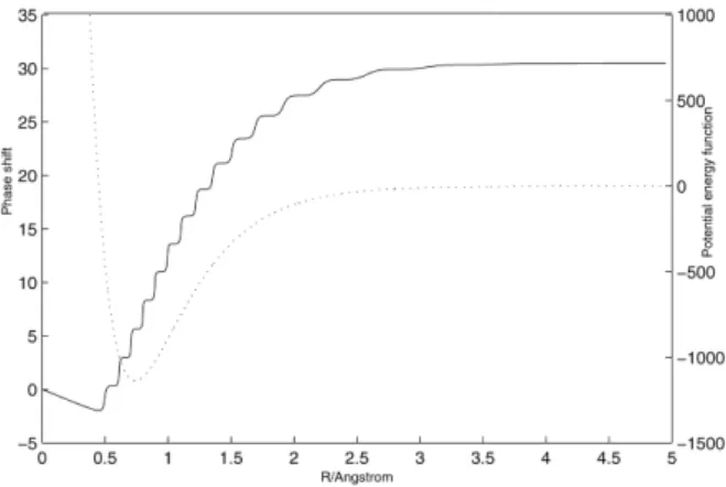
Phase shift convergence against the scattering coor-dinate is shown in Fig. 1. If the potential is positive, the phase shift will be negative. From Eq. (8) one may infer the sign of the phase shift, because it is pro-portional to−Ep(R). If an approximation is used for
the phase shift derivative, one can write that for Eq. (8),δ(R+h)≈δ(R)−U(kR)sin
2(kR+δ). Then, for a
positive potential energy function, the phase shift, to-gether with the initial condition, will give negative val-ues. However, if the potential changes sign, the phase shift will also carry this information, as exemplified in Fig. 1. The potential energy function changes sign at
R = 0.46 ˚A, exactly at the point at which the phase shift changes its behaviour. The constant phase shift value for largeR, shown in Fig. 1, is also evident from Eq. (8). In this region, the potential energy function will go to negligible values and, consequently, dδ
dR ≈0.
Figure 1 - Phase shift (full line) and potential energy function in atomic units (dashed line) plotted scattering coordinates. The parameters used in the phase shift calculations werel= 0 and
k2= 25 ˚A−2.
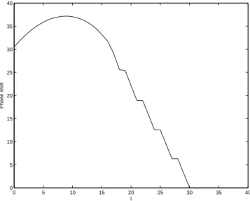
As the angular momentum is increased, the cen-trifugal term will become more important, making the potential energy function negligible. Hence, the total potential for large angular momentum will be approx-imately given by the centrifugal contribution. In this case, phase shift must go to zero, because the reference potential in the present formulation is the centrifugal potential. In fact, that is the reason for subtracting the phase−lπ2 from the computed phase shift. At
Fig. 2. This maximum angular momentum can be esti-mated from a classical analysis. The maximum impact parameter,b, above which there will be no scattering, can be estimated to be equal to the potential range,
Rmax. Because total angular momentum is given by
L = bk, one has lmax ≈ Rmaxk. Considering the
po-tential range to be 6 ˚A one haslmax≈6× √
25 = 30, as confirmed numerically. Additionally, this maximum angular momentum estimation is important to calcu-late cross section because it will involve a summation on phase shifts for different angular momenta.
Oscillations in Fig. 2 can also be explored to clar-ify the connection between classical and quantum scat-tering. In a semiclassical context, the derivative of the phase shift is proportional to the scattering angle. For this reason, the maximum in Fig. 2 corresponds to a concentration of trajectories, and consequently, greater intensity in the differential cross section, an ef-fect known as the rainbow efef-fect in atomic and molec-ular collision [13].
0 5 10 15 20 25 30 35 40 0
5 10 15 20 25 30 35 40
l
Phase shift
Figure 2 - Phase shift convergence for several angular momenta andk2= 25 ˚A−2.
Levinson’s theorem [6] states that at the limit of zero collision energy the phase shift is a multiple ofπ,
lim
k→0δ=nbπ, (13)
in which nb is the number of bound states that the
molecule can support. If there are bound states with zero energy and angular momentum different from zero, then Eq. (13) has to be modified to limk→0δ =
(nb+12)π[5,6]. As confirmed numerically, these bound
states with zero energy were not detected here. Equa-tion (13) is thus used in the present study.
Levinson’s theorem is a powerful and elegant the-orem that makes a connection between the continuum and the discrete states of system. The variable phase equation is appropriate to investigate this theorem nu-merically. Because the energy will be small, only zero
angular momentum has to be considered. Numerical integration will provide information on the number of bound states, and because transitions in infrared spec-tra are due to vibrational mode excitation, one can infer consequences, such as the number of lines, about the in-frared spectrum [10]. The results are shown in Table 2. There is a clear tendency to show that the prototype molecule can accommodate 14 bound states. In fact, at the limit fork2= 10−4˚A2, it was found that δ
π = 13.98,
confirming this tendency. Thus, the prototype poten-tial represents a molecule with 14 bound states. This procedure is the same as the procedure adopted for a realist potential energy function and was used to detect bound and meta-stable states of rare gas hydrides [5].
Table 2 - Numerical solution of Levinson’s theorem.
k2 δ
π
25 9.7
2.5 12.34 0.25 13.42
Further theoretical and computational aspects of the method can be explored. For example, the first Born approximation [6] is a special case of the variable phase method. For small phase shift values, such that sin2(kR+δ)≈sin2(kR) is a valid approximation, the phase differential equation reduces to
dδ dR ≈ −
U(R)
k sin 2(
kR) (14)
which is the first Born approximation in differential form. Integration of this differential equation gives the usual presentation for this approximation, δ ≈ −∫0∞
U(R)
k sin
2(kR).Thus, usage of the variable phase
approach can provide a simple and convincing proof of the first Born approximation.
6.
Conclusion
In contrast with numerical methods to calculate elastic scattering that require knowledge of Bessel functions, a simple approach based on the variable phase method was discussed. The algorithm discussed is very sim-ple to imsim-plement and allows several important conse-quences to be explored. Calculation of the scattering matrices were conducted and compared with results obtained using the Renormalized Numerov method. Phase shift behaviour as a function of energy and angu-lar momentum was discussed, together with numerical examples of Levinson’s theorem.
The variable phase method as presented here can be explored further to calculate other quantum properties.
Acknowledgment
References
[1] P.M. Morse and W.P. Allis, Phys. Rev.44, 269 (1933).
[2] G.F. Drukarev,The theory of Electron-Atom Collision
(Academic Press, London, 1965).
[3] F. Calogero,Variable phase approach to potential scat-tering(Academic Press, New York, 1967).
[4] R. Martinazzo, E. Bodo and F.A. Gianturco, Comput. Phys. Commun.151, 187 (2003).
[5] J. P. Braga and J.N. Murrell, Molecular Physics 53, 295 (1984).
[6] C.J. Joachain, Quantum collision theory (North-Holland, Amsterdam, 1975).
[7] J.N. Murrell and S.D. Bosanac, Introduction to the Theory of Atomic and Molecular Collisions(John Wi-ley, Chichester, 1989).
[8] J.P. Braga, J. Comput. Chem.10, 413 (1989).
[9] P.M. Morse, Phys. Rev.34, 57 (1929).
[10] G. Herzberg, Molecular Spectra and Molecular Struc-ture(Van Nostrand Reinhold, New York, 1950).
[11] B.R. Johnson, J. Chem. Phys.67, 4086 (1977).
[12] G.E. Forsythe, M.A. Malcolm and C.B. Moler,
Computer Methods for Mathematical Computations
(Prentice-Hall, Englewood Cliffs, 1977).