Available online at www.ispacs.com/cna Volume 2012, Year 2012 Article ID cna-00117, 7 pages
doi:10.5899/2012/cna-00117 Research Article
Heisenberg uncertainty relation and statistical
measures in the square well
R. L´opez-Ruiz1∗, J. Sa˜nudo2
(1)Department of Computer Science, Faculty of Science, Universidad de Zaragoza, 50009 - Zaragoza, Spain (2)Department of Physics, Faculty of Science, Universidad de Extremadura, 06071 - Badajoz, Spain
Copyright 2012 c⃝R. L´opez-Ruiz and J. Sa˜nudo. This is an open access article distributed under the Creative Commons Attribution License, which permits unrestricted use, distribution, and reproduction in any medium, provided the original work is properly cited.
Abstract
A non stationary state in the one-dimensional infinite square well formed by a combination of the ground state and the first excited one is considered. The statistical complexity and the Fisher-Shannon entropy in position and momentum are calculated with time for this system. These measures are compared with the Heisenberg uncertainty relation, ∆x∆p. It is observed that the extreme values of ∆x∆p coincide in time with extreme values of the other two statistical magnitudes.
Keywords: Statistical complexity; Fisher-Shannon entropy; Square well; Ground states
1
Introduction
The behavior of the statistical complexity in time-dependent systems has not been broadly investigated. In a previous work [1], we have studied the statistical complexityC
in a simplified time-dependent system ρ(x, t) composed of two one-dimensional (variable
x) identical densities that travel in opposite directions with the same velocity. The analysis ofCwas done for two Gaussian, rectangular, triangular, exponential and gamma traveling densities. Specifically, the shape ofρ(x, t) presenting the maximum and minimumC was explicitly shown for all these cases. In this direction, other time-dependent systems have been worked out. For instance, in [2], a gas decaying toward the asymptotic equilibrium state was studied. It was found that this system goes towards equilibrium by approaching
the maximum complexity path, which is the trajectory in distribution space formed by
the distributions with the maximal complexity. Then, from a physical point of view, it
can have some interest to study the extremal behavior of statistical magnitudes in time dependent systems.
An important statistical magnitude in quantum mechanics is the Heisenberg uncer-tainty relation ∆x∆p, which quantifies the product of the spread ∆ in the two conjugate variables, the spacexand the momentump, for a wave function. This magnitude presents some similarity with the statistical complexity and Fisher-Shannon information that are also calculated as the product of two statistical quantities, one of them representing the information content of the system, and the other one giving an idea of how far the system is from the equilibrium.
In this work, we calculate these statistical quantities on a simple time-dependent quan-tum system, specifically one composed by a linear combination of the ground state and the first excited of the one-dimensional square well. The extreme values of these magnitudes are identified and compared among them. Finally the conclusions are established.
2
The time-dependent quantum system
Let us consider a particle in a box confined in the one-dimensional interval [0, a], that is, a particle constrained in an one-dimensional infinite square well of length a. The eigenvalues of the energy for this system are given by [3]
En=
n2π2~2
2ma2 n= 1,2, . . . (2.1)
and the corresponding non-degenerate states are represented by the wave functions
ϕn(x) =
√
2
a sin (nπx
a )
. (2.2)
In order to study the time variation of the statistical magnitudes we must consider a non-stationary state. For simplicity, let us take that one formed at time t = 0 by the normalized linear combination of the ground state (n= 1) and the first excited one (n= 2)
Ψ(x, t= 0) = √1
2 (ϕ1(x) +ϕ2(x)). (2.3) Up to a global phase factor, this state evolves in time in a periodic motion expressed in the the following manner:
Ψ(x, t) = √1 2
(
ϕ1(x) +e−iwtϕ2(x)
)
, (2.4)
where the angular frequency wof the oscillation is given by
w= E2−E1
~ =
3π2~
2ma2. (2.5)
The probability density of this state in position space is:
ρ(x, t) =|Ψ(x, t)|2 = 1 2
(
ϕ21(x) +ϕ 2 2(x)
)
+ϕ1(x)ϕ2(x) cos(wt), (2.6)
and in momentum space is:
0 1 2 3 4 5 6 0.75
1.00 1.25 1.50 1.75
x
p
t
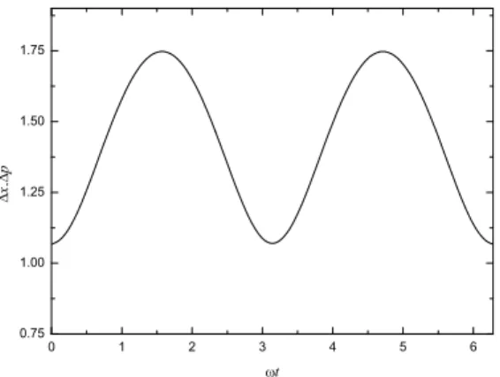
Figure 1: Heisenberg uncertainty relation ∆x∆p versus time for the state Ψ(x, t) considered in the text.
where ˆΨ(p, t) is the Fourier transform of Ψ(x, t).
Let us remark that ρ(x, t) presents the space-time symmetry
ρ(x, t) =ρ(a−x, t+π
ω )
. (2.8)
This symmetry implies that all the integral quantities calculated in the interval [0, a] with functions F(ρ) depending on the probability density ρ display a period equal to πw, as it can be easily checked from the expression
∫ a
0
F(ρ(x, t))dx=
∫ a
0
F(ρ(x, t+ π
ω ))
dx. (2.9)
A similar symmetry property can also be checked forγ(p, t) in the momentum space. Now we proceed to calculate for this system the Heisenberg uncertainty relation, the statistical complexity and the Fisher-Shannon information.
3
Calculation of the statistical magnitudes
The Heisenberg uncertainty relation ∆x∆p is found by computing the quantities
∆x = ( < x2
>−< x >2)12
, (3.10)
∆p = (
< p2 >−< p >2)12
, (3.11)
where< f >means the average value off for the specific wave function we are considering. In the case of the state given by Eq. (2.4), ∆p is constant in time, ∆p = ~π
a
√
3 2. The
result for the uncertainty relation,
∆x∆p= ~ 2
( π2
2 − 15
8 −6
(
16 9π
)2
cos2(wt)
)1 2
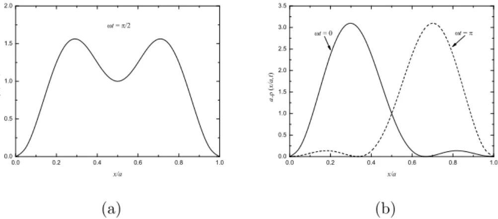
0.0 0.2 0.4 0.6 0.8 1.0 0.0 0.5 1.0 1.5 2.0 a ( x / a ,t ) x/a t = /2
0.0 0.2 0.4 0.6 0.8 1.0 0.0 0.5 1.0 1.5 2.0 2.5 3.0 3.5 t = a ( x / a ,t ) x/a t = 0
(a) (b)
Figure 2: Plot of ρ(x, t) in adimensional units with extreme values in the uncertainty relation ∆x∆p: (a) the maximum is taken att= π
2w, and (b) the minimum is taken att= 0 and t= π w.
is plotted in Fig. 1. Observe that ∆x∆p presents a periodicity with period t = wπ, and that it shows two extreme values, a maximum and a minimum, taken att= 2πw and t= 0
or wπ, respectively. The probability density ρ for these extreme values is represented in Fig. 2.
The statistical complexity C [4], the so-called LM C complexity, is defined as
C=H·D , (3.13)
where H represents the information content of the system and D gives an idea of how much concentrated is its spatial distribution. As quantifier of H we take the simple exponential Shannon entropy [5, 6], that in the position and momentum spaces takes the form, respectively,
Hx=eSx , Hp=eSp , (3.14)
whereSx and Sp are the Shannon information entropies [7],
Sx =−
∫
ρ(x, t) logρ(x, t)dx , Sp=−
∫
γ(p, t) logγ(p, t)dp . (3.15)
The disequilibrium introduced in [4, 6] is given by
Dx =
∫
ρ2(x, t)dx , Dp =
∫
γ2(p, t)dp . (3.16)
Then, the final expressions forC in position and momentum spaces are:
Cx=Hx·Dx , Cp =Hp·Dp . (3.17)
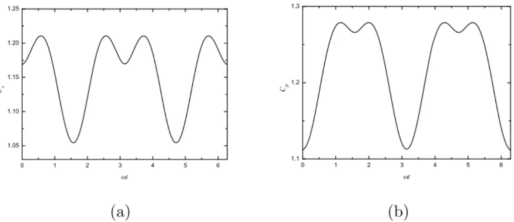
The plots of Cx and Cp are shown in Fig. 3. Observe that both magnitudes display
relative minima at t = 2πw and t = πw, just on the points where the uncertainty relation also presents relative extrema, although in this case they are maximum and minimum, respectively.
Another statistical measure that has been used in quantum systems [8, 9] is the Fisher-Shannon information P. This quantity, in the position and momentum spaces, is given respectively by
0 1 2 3 4 5 6 1.05
1.10 1.15 1.20 1.25
C
x
t
0 1 2 3 4 5 6
1.1 1.2 1.3
C
p
t
(a) (b)
Figure 3: Statistical complexity versus time for the state Ψ(x, t) considered in the text: (a) in position,Cx, and (b) in momentum,Cp.
0 1 2 3 4 5 6
2.75 3.00 3.25 3.50 3.75
P
x
t
0 1 2 3 4 5 6
0.02 0.03 0.04 0.05 0.06 0.07
P
p
t
(a) (b)
Figure 4: Fisher-Shannon entropy versus time for the state Ψ(x, t) considered in the text: (a) in position,Px, and (b) in momentum,Pp
where the first factor
Jx =
1 2πe e
2Sx/3, J
p =
1 2πe e
2Sp/3, (3.19)
is a version of the exponential Shannon entropy [5], and the second factor
Ix =
∫ [
∇xρ(x, t)]2
ρ(x, t) dx , Ip =
∫ [
∇pγ(p, t)]2
γ(p, t) dp , (3.20)
is the so-called Fisher information measure [10], that quantifies the narrowness of the probability density.
The plots of Px and Pp are shown in Fig. 4. Observe that both magnitudes display
4
Conclusions
The Heisenberg uncertainty relation has been calculated for a time-dependent quantum system in the one-dimensional square well, specifically the normalized linear combination of the ground state and the first excited one. This relation has a periodic behavior in time with period π/w, and shows two extrema values that are taken at t = π/(2w) the maximum, and at t= 0 or t =π/w the minimum. Similar properties of periodicity and extreme values are observed for the behavior of other statistical magnitudes, namely the statistical complexity and the Fisher-Shannon information, that have been computed in position and momentum spaces.
Acknowledgments
The authors thank the referees for useful comments and suggestions. This research was supported by the spanish Grant with Ref. FIS2009-13364-C02-C01. J.S. also thanks to the Consejer´ıa de Econom´ıa, Comercio e Innovaci´on of the Junta de Extremadura (Spain) for financial support, Project Ref. GRU09011.
References
[1] R. Lopez-Ruiz, J. Sa˜nudo, Shape of traveling densities with extremum statistical complexity, Int. J. Appl. Math. Stat. 26 (2012) 81-91.
[2] X. Calbet, R. Lopez-Ruiz, Tendency toward maximum complexity in a non-equilibrium isolated system, Phys. Rev. E 63 (2001) 066116, 9 pages.
[3] C. Cohen-Tannoudji, B. Diu, F. Laloe, Quantum Mechanics, 2 vols., Wiley, New York, 1977.
[4] R. Lopez-Ruiz, H.L. Mancini, X. Calbet, A statistical measure of complexity, Phys. Lett. A 209 (1995) 321-326.
http://dx.doi.org/10.1016/0375-9601(95)00867-5
[5] A. Dembo, T.A. Cover, J.A. Thomas, Information theoretic inequalities, IEEE Trans. Inf. Theory 37 (1991) 1501-1518.
http://dx.doi.org/10.1109/18.104312
[6] R.G. Catalan, J. Garay, R. Lopez-Ruiz, Features of the extension of a statistical measure of complexity to continuous systems, Phys. Rev. E 66 (2002) 011102, 6 pages.
[7] C.E. Shannon, A mathematical theory of communication, Bell. Sys. Tech. J. 27 (1948) 379-423.
[8] E. Romera, J.S. Dehesa, The FisherShannon information plane, an electron correla-tion tool, J. Chem. Phys. 120 (2004) 8906-8912.
[9] H.E. Montgomery Jr., K.D. Sen, Statistical complexity and FisherShannon informa-tion measure ofH2+, Phys. Lett. A 372 (2008) 2271-2273.
http://dx.doi.org/10.1016/j.physleta.2007.11.041
[10] R.A. Fisher, Theory of statistical estimation, Proc. Cambridge Phil. Soc. 22 (1925) 700-725.