Samantha Haussmann Universidade Federal de Minas Gerais André Braz Golgher Universidade Federal de Minas Gerais
Resumo
Como comumente apontado pela literatura sobre as diferenças salariais por sexo, em geral, ho-mens recebem mais que mulheres em ocupações similares. Entretanto, algumas tendências atuais no Brasil mostram que os hiatos no mercado de trabalho entre os gêneros estão diminuindo em di-versos aspectos.Esse artigo analisa essa questão empiricamente fazendo uso de PNADs, equações Mincerianas e modelos hierárquicos baseados na abordagem Idade-Período-Coorte. Uma das conclusões principais do artigo é que apesar das mulheres terem salários menores que os homens para ocupações, locais de residência e níveis edu-cacionais similares, os atributos femininos asso-ciados ao mercado de trabalho e a diminuição na segregação ocupacional parcialmente compensam essa vantagem não explicada dos homens. Além disso, depois de controlados os efeitos por coorte, observa-se uma convergência entre os gêneros e verifica-se que muitos dos hiatos são não signi-ficativos.
Palavras-chave
mercado de trabalho; gênero; Brasil.
Códigos JELJ31; J70. Abstract
Labor market literature attests that men tend to earn more than women in similar occupations in Brazil and elsewhere. However, some recent trends that have occurred in Brazil promote the narrowing of gender gaps in the labor market. This paper analyzes this issue empirically with the use of PNADs, Mincerian wage equations, and a hierarchical model based on the Age-Period-Cohort approach. We observed that gender wage gaps were shrinking and, although there might still be an unexplained advantage for men in the labor market, the evolution of women’s endowments for the labor market and the decrease in labor market segregation significantly compensated for this difference. Due to these trends, after controlling for cohort differences, we observed non-significant gender wage gaps in some models.
Keywords
labor market; gender; Brazil.
JEL CodesJ31; J70.
Shrinking gender wage gaps in the Brazilian
labor market:
an application of the APC
approach
1
Introduction
Labor market literature attests that men tend to earn more than women in similar occupations in Brazil and elsewhere (Camargo; Serrano, 1983; Barros et al., 2001; Arabsheibani; Carneiro; Henley, 2003; Leme; Wajnman, 2000; Madalozzo, 2010; Ñopo, 2012a,b; Weichselbaumer; Winter-Ebmer, 2003). The concentration of women in low-paid occupations and the exis-tence of gender wage gaps have several plausible explanations, some of which we describe below.
In traditional societies, it is more common for women than for men to
withdraw temporarily from the labor market or to choose jobs with flexible
schedules and/or with fewer working hours. Women’s main reasons for doing so arise from housework and childcare responsibilities. Consequently, wo-men accumulate less labor market experience than wo-men do, and wowo-men tend to invest less in education and on-the-job training, as they anticipate shorter and more discontinuous work lives (Blau; Khan, 2000; Madalozzo, 2010).
Other factors, such as labor legislation, maternity leave and pregnancy protection, may increase women’s labor costs, impact negatively on fema-les’ wages (Madalozzo, 2010), and decrease the employability of women (Blau; Khan, 2000). Occupational segregation and discrimination against women might also be important in determining relative wages (Blau; Khan, 2000; Oliveira, 1997; Leme; Wajnman, 2000; Ñopo, 2012a,b)
However, some recent trends might change this perspective on females’ disadvantages in the labor market. For instance, there was an increase in the participation of females in the labor market, while the participation of men was, at most, stable in recent decades (Juhn; Potter, 2006; Wajman; Rios-Neto, 2000). This indicates that the labor market is becoming a more female locus, with a relative increase in females’ experience vis-à-vis that of males, a feature that might positively affect many women’s outcomes in traditional labor markets.
impact on females’ available time to invest in the labor market, increasing women’s competiveness. In addition, lower fertility rates reduce the cost of female labor by reducing the demand for maternity leave (Madalozzo, 2010).
However, women tend to be more household-focused than men and are still responsible for most domestic tasks. For instance, Bruschini (2006) analyzed the amount of time spent by males and females on domestic chores in Brazil, in 2002. She concluded that the time spent by women was much greater than that spent by men. However, household chores are becoming lighter and more evenly distributed among the sexes (Juhn; Potter, 2006), and consequently, women’s time availability potentially em-ployed in the labor market increased (Madalozzo, 2010), especially among
more qualified females, as differences between sexes decreased for more educated individuals (Bruschini, 2006).
In addition, divorce rates increased and, as divorced women tend to participate more in the labor market, this promoted an increase in fema-les’ labor market participation (Fernández; Wong, 2011). Furthermore, the end of the widely held societal understanding of marriage as a lifelong in-vestment (Amato; Rogers, 1999) relatively increases the value of women´s labor market investments in formal education and on-the-job training, re-sulting in higher productivity and wages vis-à-vis men.
Moreover, the service sector’s increasing share of the economy, which created more labor demand in occupations well suited to women, helped females to gain access to many better-paid types of occupations (Juhn; Potter, 2006). Traditional societies relied on many agricultural and manual jobs which required a high degree of physical strength. In contrast, most current jobs are less physically demanding, but they require other attribu-tes, such as patience and dexterity, in which females do not have disad-vantages when compared to men (Blau; Kahn, 2000).
In Brazil, females tend to have higher schooling levels than men, and differences are increasing (Whinter; Golgher, 2010). This might positively influence women’s labor market participation, as education and participa-tion are positively correlated. Besides, this surely will promote an increase in the proportion of female participation in qualified jobs, decreasing occu-pational segregation (Blau; Kahn, 2000; Madalozzo, 2010).
bar-gaining power (Jensen, 2012). Due to circular causality, these features might create virtuous cycles between labor market participation and social norms, promoting further advances in women’s relative labor market positions.
Due to these trends, and as emphasized by Juhn and Potter (2006), women’s choices regarding human capital investments, marriage and ferti-lity shape females’ values and roles in the labor market and in society, pro-moting changes over their life course. Moreover, as young women reach working age, they will probably make pro-labor market decisions and li-felong career plans more frequently than older cohorts did. Because of all these trends, females’ labor market participation rapidly improved both quantitatively and qualitatively in Brazil relative to men’s participation (Barros, 2001): wage and labor market participation gaps and labor market segregation decreased, and a convergence between sexes was observed.
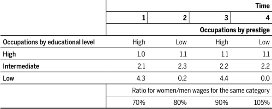
In order to clarify the main objective of this paper, we present in Table 1 some hypothetical examples of gender wage gaps and labor market parti-cipation by educational level and occupational prestige. The table presents four situations, from time 1 to time 4, which can be viewed as a path from males’ to females’ supremacy in the labor market. In each situation,
occupations are classified in three categories of educational level and two of prestige. At each time, there are ten men and ten women in the labor market, who are distributed in each of the six possibilities of education and prestige: the first number is for men and the second for women. For instance, in time 1, one man was classified as having an occupation of high education and high prestige and no women were in this category. At this same time, four men had positions classified as low educational level and high prestige, and three women were in this same category. Moreover, in time 1, women earned 70% as much as men in occupations of similar educational level and prestige.
Table 1 Hypothetical examples of gender wage gaps and labor market participation by educational level and occupational prestige.
Time
1 2 3 4
Occupations by prestige
Occupations by educational level High Low High Low
High 1.0 1.1 1.1 1.1
Intermediate 2.1 2.3 2.2 2.2
Low 4.3 0.2 4.4 0.0
Ratio for women/men wages for the same category
70% 80% 90% 105%
This paper analyzed labor market gaps between sexes in Brazil taking into account that educational levels and labor market segregation varied re-cently. In the empirical analysis, we used the National Household Sample Surveys (in Portuguese: PNAD - Pesquisa Nacional por Amostra de Domi-cílios) of 1992, 1997, 2002, 2007 and 2012. Concerning our econometric strategy, we initially estimated Mincerian wage equations using OLS with different sets of controls. The objective is to analyze gender wage gaps with and without controls associated with education and labor market segregation. We began with the classical analysis of gender wage gaps with many controls, that is, the traditional approach of comparing men and women in similar occupations and educational levels, and then we dropped some of the controls in order to analyze gender wage gaps taking into account that educational levels and labor market segregation varied over the period.
During the studied period, expectations about women’s roles in society radically changed (Juhn; Potter, 2006). In order to apprehend the age, pe-riod and cohort effects of labor market trends and evolution, we used a hierarchical model based on Age-Period-Cohort approach. The objective is to focus the analyses on cohorts, as cross-section analysis might be mis-leading (Leme; Wajnman, 2000; Wajnman; Rios-Neto, 2000). To the best
of our knowledge, this is the first attempt to analyze gender wage gaps in the Brazilian labor market using this methodology.
pa-per. The fourth presents some descriptive statistics regarding labor market trends in Brazil, giving an overall perspective on labor market evolution
with emphasis on sex differentials. The fifth section describes the applied methodology. Initially we present the databases, then we discuss the Min-cerian equations and the variables used in the models, and, after this, we present the hierarchical model. The sixth section presents the results of the econometric models. The last section concludes the paper.
2
Literature review
This section presents a selection of papers that discussed gender gaps in the labor market. The objective is to give an overall description of the field, giving special attention to the Brazilian reality.
Many studies observed a tendency toward shrinking gender wage gaps in different settings (For instance, Blau; Kahn, 2000; Brown; Corcoran, 1996; Weichselbaumer; Winter-Ebmer, 2003). Blau and Kahn (2000) veri-fied a shrinking gender wage gap in the U.S.; this trend was more rapid in the U.S. until the 1990s than it was in many other European countries. Ac-cording to these authors, one of the reasons for these trends is that greater numbers of women are entering better-paid occupations that were tradi-tionally dominated by men. Moreover, these authors observed a decrease in the size of the unexplained gender gap, possibly due to an upgrading of women’s unobservable skills and/or lower levels of discrimination.
Similarly, Brown and Corcoran (1996) analyzed gender wage gaps in the U.S. and observed that one of the reasons for the closing gender gaps was the increase in female participation in better-paid occupations that were traditionally dominated by men. They noted that differences in the proportion of college graduates by field accounted for a significant part of the gender earnings gap, as women were overrepresented in careers with lower wages.
re-presenting the sexes in econometric models, and the traditional use of the Oaxaca-Blinder decomposition, and results did not differ consistently for gender wage gaps. Moreover, they noted that the gender wage gap was smaller if only a sample of new entrants in the labor market was investiga-ted or if only high-prestige jobs were analyzed.
In a similar vein, Manning and Swaffield (2008) emphasized that cross--section data confound true life-cycle effects and cohort effects. They ob-served that the gender pay gap between sexes in the UK was approxima-tely zero upon entry into the labor market, but it grew afterwards. They explored three main hypotheses to explain why the gap between men and women grew over time. Human capital factors - gender differences in accumulated work experience, investments in human capital and do-mestic commitments - explained approximately 50% of the gap. The job--shopping hypothesis, which states that an important part of early career wage growth is associated with moving from worse to better-paying jobs, explained around 6% of the gap. Psychological differences between men’s and women’s attitudes toward risk-taking, competition, self-esteem, and selflessness at the age when they enter the labor market accounted for up to 20% of the gap.
ca-reer investments, decreasing labor market gaps (Bailey; Hershbein; Miller, 2012). Fernández and Wong (2011) observed that gender gaps in labor par-ticipation fell remarkably and that changes in divorce probabilities alone accounted for more than half of these trends.
Arulampalam, Booth and Bryan (2007) emphasized that, although gen-der wage gaps have been widely studied, as in the studies described abo-ve, it was only relatively recently that analysis has been performed across the wage distribution, which overcomes some of the limitations of the usual methodology. In this vein, García, Hernández and López-Nicolás (2001) used quantile regressions (QR) to analyze gender wage differences in Spain across the wage distribution. They observed that gender wage gaps were greater for the highest quantiles, although differences between quantiles were not great and standard errors were large. Arulampalam, Booth and Bryan (2007) applied the QR approach to European data. They
defined that a glass ceiling effect existed if the 90th percentile wage gap
was larger than the wage gaps in other parts of the wage distribution by at least two percentage points. They observed that most countries showed this effect. Similarly, Albrecht, Bjorklund and Vroman (2001) analyzed data for Sweden and observed a glass ceiling effect in the 1990’s, but not in prior decades. Rica, Dolado and Llorens (2008) used a similar approach applied to the Spanish data, and observed this pattern for highly educated workers, but not for less-educated ones.
Some other authors discussed data from Latin America and/or Brazil. Ñopo (2012a) analyzed the evolution of gender earning gaps in Latin America. The author points out that, although women are overrepresen-ted in low-paid occupations, the general distribution of observable cha-racteristics favors women when compared to men, indicating that the unexplained part of the gender earning gap is remarkable. Nevertheless, the author observed that both explained and unexplained gender gaps decreased recently.
After this first study regarding gender labor market gaps in Brazil, many others followed. For instance, Leme and Wajnman (2000) observed a de-crease in gender wage gaps using PNADs and the Oaxaca decomposition. They observed that the increase in women’s educational levels, associa-ted with relatively greater returns for these attributes and a decrease in discrimination against women, had a positive impact on females’ wages vis-à-vis males’. In addition, younger cohorts obtained greater returns for their human capital investments, suggesting further positive impacts on females’ wages in the long run.
Barros et al (2001) emphasized that, although men still tended to earn more and to work in greater proportion and for more hours than women, females’ labor market participation rapidly improved both quantitatively and qualitatively. Moreover, they observed that, while there was a clear labor market segregation by sex, traditional female occupations showed similar wages to those in which men had historically predominated.
Arabsheibani, Carneiro and Henley (2003) also analyzed gender wage differentials in Brazil. They used PNADs and the Juhn, Murphy and Pier-ce (JMP) decomposition. The authors observed that gender wage gaps decreased mostly due to lower levels of discrimination against women. Moreover, they emphasized that some other trends had a positive impact on narrowing these gaps. For instance, the positive evolution of females’ observable earning-improving endowments, such as human capital level, and also of non-observables, such as effort, relatively increased women’s wages vis-à-vis men’s.
Silva, Carvalho and Neri (2006) analyzed wage differentials between gender and race using the 2003 PNAD and the Oaxaca and Heckman pro-cedures. They concluded that white men earned more than other groups, in part due to discrimination.
Madalazzo (2010) also observed narrowing gender wage gaps in Brazil from 1978 to 2007. She observed that labor market segregation decrea-sed for careers traditionally dominated by men, while women continue to dominate those occupations considered female. According to the author, given that the first type of occupation tends to pay better wages, this fact positively influenced the convergence of wages between the sexes.
the largest proportion of variability was unexplained; the unexplained por-tion is normally linked to discriminapor-tion in the labor market. He observed that women would earn more than men if the unexplained portion of wage gaps did not exist, as women had better earning-improving endowments.
The author also verified that gender earning gaps increased with age for young cohorts, and that younger cohorts showed smaller gender gaps.
Salardi (2014) analyzed the evolution of gender occupational segrega-tion in the Brazilian labor market between 1987 and 2006. She observed that gender segregation has fallen during this period, mostly due to a decli-ning concentration by gender within individual occupations.
All these studies that analyzed the Brazilian reality pointed to a con-vergence in labor market outcomes by sex. The current paper is similar in many aspects to those discussed above; however, besides being a more updated study, it is founded on a different theoretical perspective and on a distinct methodology, which are based on the Age-Period-Cohort (APC) approach. This approach is described in the next section.
3
The Age-Period-Cohort (APC) approach
This paper develops the exercise of placing labor market outcomes in a life course perspective, using as theoretical background the APC approach. In this approach, age, period, and cohort effects are analyzed separately in order to disentangle their distinct contributions, as briefly described below. For a more detailed discussion see Mason and Smith (1985), Yang, Fu and Land (2004), Yang and Land (2008), Yang et al. (2008) and Yang (2008, 2011).
When changes that take place in a society affect a specific age group (or groups) most strongly, the result is an age effect, aging-related developmen-tal changes that occur in life. In this case, one would observe that certain age groups, regardless of their cohort or period, share the same characte-ristics or face the same phenomena. Puberty is a classic example of an age effect. Another example of this could be the probability of older people being more satisfied with life than youngsters.
econo-mic crisis of 1929 and the terrorist attacks of 2001 in the United States are examples of period effects that are likely to affect the society in which they occur as a whole.
Finally, cohort effects refer to individuals who share specific experiences, such as being born in the same year or entering a university in the same period. According to Ryder (1965), birth cohorts represent the effect of for-mative experience, shaped not only by life conditions from the moment of birth but also by a continuous and shared exposure to historical and social factors that might affect living conditions throughout life, thus making the specific group unique. For instance, individuals of specific cohorts might trust others less than other cohorts, independently of age or period effects. The APC approach can be applied by different methods. Ideally, one would prefer to work with databases that follow the same individual over time. However, in the absence of longitudinal data to investigate long-term changes in Brazil, we built cohorts using five different PNADs. As described in the methodological section, recently developed statistical tools transform cross-sectional data, such as those provided by PNADs, into well-grounded synthetic cohorts that mimic true birth cohorts (Yang, 2008).
4
Empirical strategy
In this section, we present the methodology in three brief subsections. The first one describes the databases, the second, the Mincerian models and the variables, and the last, the hierarchical model based on APC approach.
4.1 Database
We used the databases from the years of 1992, 1997, 2002, 2007 and 2012. The last one was the most recent available at the time of this
re-search. The others come in five-year intervals so we could easily build cohorts with the databases. The objective was to have enough time span to comprehend the recent evolution of the Brazilian labor market.
Given the study’s objective of analyzing labor market outcomes, we selected individuals from 20 to 69 years old with positive income. Our final sample sizes in the five mentioned years were respectively 102096, 116126, 136907, 152764 and 145050.
In order to build the cohorts, we initially selected women between the ages of 20 and 54. The upper limit was selected because older women show a much greater propensity to retire, so the women remaining active in the labor market would be highly self-selected. Then we classified the individuals into five-year age groups. For some cohorts, we did not have the data for all years. Those cohorts were discarded from some of the analysis. Hence, we obtained three cohorts with data in all five PNADs. The youngest cohort was 20 to 24 years old in 1992 and, consequently, 40 to 44 years old in 2012. The other cohorts with complete data were res-pectively 5 and 10 years older. Thus, the oldest cohort with data in all five PNADs was 30 to 34 years old in 1992 and, consequently, 50 to 54 in the end of the period. We also defined two other cohorts which did not have data for all years: those aged 10 to 14 and 15 to 19 in 1992.
4.2 Mincerian models and variables
The Mincerian wage equations are commonly used to analyze the rela-tionship between salaries and other variables, such as sex, age and race (Resende; Wyllie, 2006; Madalazzo, 2010). This type of model is exten-sively used in many applications and settings. For instance, Sachsida, Loureiro and Mendonça (2004) used this econometric model to analyze Brazil and Trostel, Walker and Woolley (2002) used it do study other countries. For an overview of Mincerian equations see Heckman, Loch-ner and Todd (2003). For a comparison of this method with other ap-proaches see Weichselbaumer and Winter-Ebmer (2003).
expla-natory variables are commonly used in Mincerian models and detailed afterwards:
where Y is hourlywage, βS are the estimated coefficients, the explanatory
variables are briefly named above, and ε is the normally distributed
sto-chastic error.
The dependent variable is the logarithm of hourlywage, as commonly used in similar analysis (For instance, see Khamis, 2008).
Many studies analyze gender wage gaps using a dummy variable for sex. Another widespread applied methodology is the use of separate equa-tions for each sex and a subsequent decomposition by Oaxaca-Blinder or other methods (Weichselbaumer; Winter-Ebmer, 2003). We chose to use the dummy variable approach (1 – Male, 0 – Female) as an initial study that is complemented by the hierarchical models and the APC approach.
Some variables are commonly used as controls in Mincerian equations (See Heckman, Lochner and Todd (2003) for a general discussion). The models used in this paper include a dummy for ethnic group (1 – White/ Asian, 0 – Black/Brown/Indigenous), as differences are envisaged between these groups. We expect a positive coefficient, as observed in Arabsheiba-ni, Carneiro and Henley, 2003.
Age is proxy for experience and is represented by a continuous variable. Age-squared is also included in the model in order to account for non--linearities. Experience is also measured using as proxy the result of age – 6 – number of years in school. However, we believe that many Brazilians acquire working experience while in school; therefore we did not account for the number of years in school while building our explanatory variable. We expect a positive coefficient for the first and a negative for the second, as wages tend to increase more quickly in the beginning of professional life, as observed in Madalozzo (2010).
Another factor that might influence earnings is the relationship of the individuals in the household. For instance, it is expected that household heads earn more than other individuals in the household do, as they tend to be more focused on labor market outcomes. This tendency is more pronounced because the head is defined by the individual’s share in
8 11 12 15 16 21
. Schooling Occupational Geographical,
20 1 2 3 4 5 7
household income. Thus, the models include three dummies for spouse, for children and for other members in the household, with the reference
being the household head. Negative coefficients for all three dummies are expected.
It is well known that one of the main determinants of wage inequalities is educational level. Hence, we included four dummies for educational le-vel. We chose to use dummies due to non-linearities and varying marginal returns to education, as in Madalozzo (2010). The dummies represent those who had 4 to 7 years of formal education (upper elementary level), 8 to 10 years of education (complete elementary level or incomplete high school), 11 (high school diploma), or 12 and more (at least some tertiary level). The category 0 to 3 (no education or lower elementary level) is the reference. We expect positive signs for all of them with increasing magnitude.
Four dummies representing the type of occupation of the worker were also included in the model, as men and women tend to be segregated in the labor market (Madalozzo, 2010; Oliveira, 1997). The categories are: worker with formal documents, public worker, self-employed and emplo-yer. The reference is informal workers. We expect positive coefficients for all but the self-employed. This last group is very heterogeneous (Khamis, 2008) and we do not have a prior expectation.
There are at least two other variables in the database that could be used to further classify occupation types, which are occupational groups and sector of activity. The focus of the paper is to analyze wage gaps without con-trolling for distributional effects among occupational groups and sector of activity. Therefore, we did not include further variables for occupation types.
Given that Brazil is highly spatially heterogeneous, we also included some geographical variables, as in Arabsheibani, Carneiro and Henley (2003) and in Madalozzo (2010). The first is a dummy for urban areas and another for metropolitan areas. Positive coefficients are expected for both, as wages tend to be higher in these regions than in rural and non-metro-politan areas. Moreover, we included four dummies associated with the macroregions in Brazil: North, Northeast, South and Central-West. The Southeast region is the reference. We expect a negative coefficient for all dummies, as this last region is in many aspects the most developed in Bra-zil and tends to have the highest wages.
The proposed model does not differ much from other studies of Brazi-lian data and there is no innovation in it. The empirical strategy, however, includes some new perspectives. We estimated the models separately by year and for particular cohorts and they are the basis for further discussions using hierarchical models. We describe this model in the next section.
4.3 Hierarchical model and the age-period-cohort approach
Mincerian models enable the analysis of age, period and/or cohort effects; however, this approach has some limitations, as these three parameters have confounding aspects if used together in the same regression (Yang; Fu; Land, 2004). That happens because, by knowing one person’s age and the year of the interview, it is possible to learn his/her year of birth (or cohort). Because of the linear dependency among age, period, and cohort,
models using the APC approach might present problems of identification, which may make the assessment of the age, period, and/or cohort effects troublesome (Yang, 2011).
How can one disentangle the effects of age, period and cohort? In our
analysis, we applied a hierarchical model based on the APC approach. In many aspects, the first level of the model resembles the Mincerian equa-tions discussed in the previous subsection and the variables are mostly the same. Given the results of the descriptive section and of the Mince-rian models, and due to the expected variability in results for the different
cohorts, each cohort was analyzed separately. Notice the term αj instead
of βS, as detailed below:
Where j represents periods, and other variables have already been defined. The equation for the second level of the model is the following:
αj = π0 + τ0j Period,
Where π0 is the expected mean at the zero values of all level1 variables
averaged over all periods, and τ0j are the coefficients for periods.
21 2 3 4 5 7
ln Y j Male Ethnic Age Age Household
8 11 12 15 16 21
We applied this methodology using the SAS 9.4 statistical package and the GLIMMIX command.
5
Descriptive statistics
This section presents descriptive statistics on trends related to the Brazilian labor market and, in some aspects, is similar to Leme and Wajnman (2000), although updated. The objective is to give an overall perspective on labor market evolution with emphasis on sex differen-tials, having as background the above discussion of age, period and cohort effects.
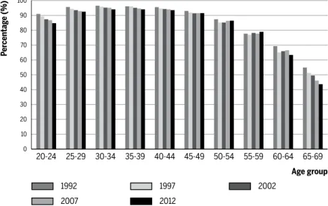
Figures 1 and 2 compare labor market participation by age, respec-tively, for males and females. These trends are well known for the Brazilian labor market (Arabsheibani; Carneiro; Henley, 2003; Leme; Wajnman, 2000; Madalozzo, 2010; Salardi, 2014; Wajnman; Rios-Neto, 2000). Many aspects of the trends in Brazil are similar to those in other countries (Juhn; Potter, 2006). Values for males are higher than for fema-les in any given age group, and dynamics differ between sexes.
Figure 1 Labor market participation for males in different age groups in different years
Source: PNAD 1992, 1997, 2002, 2007 and 2012
0 50
40
30
20
10 60 100
90
80
70
20-24 25-29 30-34 35-39 40-44 45-49 50-54 55-59 60-64 65-69
1992 1997 2002
P
er
centag
e (%)
2007 2012
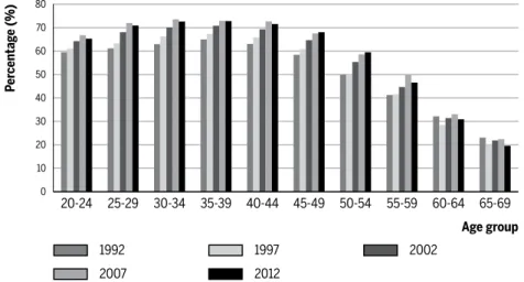
Figure 2 Labor market participation for females in different age groups in different years
Source: PNAD 1992, 1997, 2002, 2007 and 2012
Male values decreased between 1992 and 2012 in the first two age groups, suggesting that some men are postponing labor market insertion in order to enhance their schooling levels. However, at least one other phenome-non might affect these results. Many young males are simply becoming part of the triple no group: they do not study, do not work and do not look for a job (Camarano; Kanso, 2008). Labor market participation decreased in the last two age groups in the period, possibly due to earlier retirement (Glomm; Jung; Tran, 2009; Queiroz, 2006). For the other age groups, the values were reasonably stable.
For females, labor market participation increased between 1992 and 2012 in all age groups but the last. Nevertheless, values appear to have remained stable since 2007, suggesting that a limit to this increase might have been achieved. Wajnman and Rios-Neto (2000) also observed a simi-lar result and emphasized that female labor market participation will not reach North American levels in the near future. One of the reasons for this suggested limit is the sizable proportion of the female population in Brazil, around 25%, in the triple no group (Golgher, 2010).
Figure 3 shows the sex ratios for labor market participation by age group in different years. Not surprisingly, male workers were the majority in all age groups and years, as described in Figures 1 and 2. Another noticed tendency is that the values are decreasing over the period, indicating the
0 50
40
30
20
10 60 80
70
20-24 25-29 30-34 35-39 40-44 45-49 50-54 55-59 60-64 65-69
1992 1997 2002
P
er
centag
e (%)
2007 2012
relative increase in female participation. Moreover, for each specific year, the numbers remain approximately constant up to a given age – the 40-44 group in 1992 and 1997, 45 – 49 in 2002 and 2007, and 50- 54 in 2012--and then increased. This suggests that women are becoming increasingly active relative to men, especially in older groups.
Figure 3 Sex ratio for labor market participation in different age groups in different years
Source: PNAD 1992, 1997, 2002, 2007 and 2012
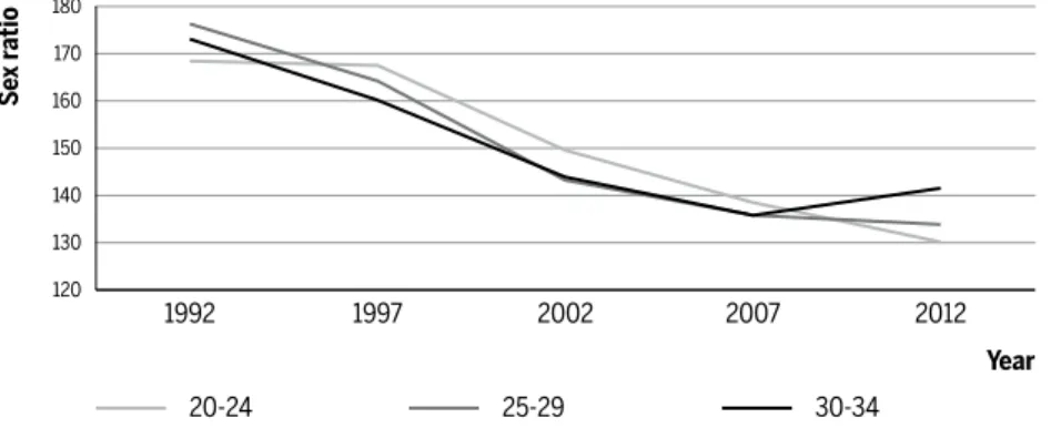
Figure 4 Sex ratio for labor market participation in different cohorts (by age in 1992) in different years
Source: PNAD 1992, 1997, 2002, 2007 and 2012
Figure 4 presents the results for labor market participation by cohort. Leme and Wajnman (2000) emphasized that the use of cohorts may be more effective than describing the data only for periods in order to analyze la-bor market outcomes. Similarly, Wajnman and Rios-Neto (2000) describe
120 220
200
180
160
140
20-24 25-29 30-34 35-39 40-44 45-49 50-54
1992 1997 2002
S
ex
r
atio
2007 2012
Age group
120 170
160 180
150
140
130
1992 1997 2002 2007 2012
20-24 25-29 30-34
S
ex
r
atio
the importance of discussing cohorts in labor market analysis. Examples of other studies that addressed labor issues with a cohort perspective are Bailey, Hershbein and Miller (2012), who analyzed the gender wage gap in the U.S., and Fernández and Wong (2011), who described trends in educa-tion and labor market participaeduca-tion in the U.S.
Figure 4 shows the results for the three cohorts with data in the five PNADs, those who were aged 20-24, 25-29 or 30-34 in 1992. Notice that there was not much difference between cohorts in each specific year: sex ratios in the labor market decreased from approximately 170 in 1992 to 135 in 2012.
The results of these two last figures indicate that women are beco-ming increasingly active relative to men, specifically due to period effects, as highlighted by the great difference in Figure 3 and the resemblance between cohorts shown in Figure 4. The period effects reflect changes in social and historical conditions of the period that affect the life of indi-viduals regardless of their age (Yang, 2011). For instance, divorce proba-bilities increased, technological change occurred in the workplace and in the household, and expectations about women’s role changed towards working women, irrespective of age or cohort. Economic crisis may also play a role as, for instance, women’s labor participation might increaseas a strategy to complement household income in particular periods. Montali (2003), for instance, discusses, for the Brazilian context, the relationship between economic restructuring and increasing unemployment and new household configurations regarding the labor market.
This descriptive analysis presented in figures 1 to 4 regarding labor par-ticipation shows that gender gaps decreased between 1992 and 2012. How
much further will they diminish? Given the trends described above, it is
likely that gaps will continue to decrease, but the pace of this decrease will slow in the future.
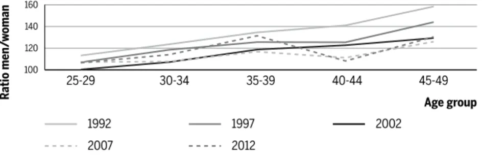
Some other trends in the labor market are also contributing to decrea-sing gender gaps. For instance, among those who work, men still work for longer hours in all age groups, as shown in Figure 5. However, differences between sexes decreased for all age groups in the period. Notice that dif-ferences for younger groups are quite small nowadays.
two cohorts, the ratio increased while women were in their twenties. That is, the age of 30 seems to be a threshold. In all cohorts, the gap in working hours between men and women increased before this age and decreased af-terwards. These trends might explain part of the divergence between sexes in wages for early career professionals, as observed by Manning and Swaffield (2008). Related to these results are some aspects associated with motherhood and time allocated to domestic activities (Bailey; Hershbein; Miller, 2012; Bruschini, 2006; Fernández; Wong, 2011; Maume; Sebastian, 2012; Tsang et al., 2003). Moreover, as women tend to study more than men do, they might spend a greater amount of time acquiring formal education, which will posi-tively affect wages in the future. That is, they are postponing earnings.
Figure 5 Ratio of number of hours spent working by men and women by age group in different years
Source: PNAD 1992, 1997, 2002, 2007 and 2012
Figure 6 Ratio of number of hours spent working by men and women, grouped by cohort by age in 1992, in different years
Source: PNAD 1992, 1997, 2002, 2007 and 2012
105 130
125
120
115
110
20-24 25-29 30-34 35-39 40-44 45-49
1992 1997 2002
R
atio o
f men/
w
omen
2007 2012
Age group
110 130
125
120
115
1992 1997 2002 2007 2012
20-24 25-29 30-34
R
atio men/
w
oman
The results presented in Figures 5 and 6 suggest that there is a remarka-ble period effect for workload gaps. Moreover, they also indicate age and cohort effects for these gaps.
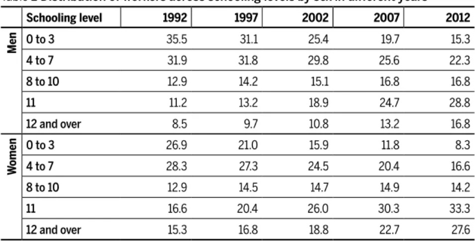
Table 2 shows the evolution of educational attainment for male and female workers in the years 1992, 1997, 2002, 2007 and 2012. In the beginning of the
period, men and women had similar distributions among the five schooling categories (0 to 3 years of formal education, 4 to 7, 8 to 10, 11 and 12 and over), although females had a slight advantage. In 2012, both genders had remarkably increased their mean levels of education; however, women’s edu-cational levels had risen more rapidly than men’s, increasing the gender gap.
Table 2 Distribution of workers across schooling levels by sex in different years
Schooling level 1992 1997 2002 2007 2012
Men 0 to 3 35.5 31.1 25.4 19.7 15.3
4 to 7 31.9 31.8 29.8 25.6 22.3
8 to 10 12.9 14.2 15.1 16.8 16.8
11 11.2 13.2 18.9 24.7 28.8
12 and over 8.5 9.7 10.8 13.2 16.8
W
omen
0 to 3 26.9 21.0 15.9 11.8 8.3
4 to 7 28.3 27.3 24.5 20.4 16.6
8 to 10 12.9 14.5 14.7 14.9 14.2
11 16.6 20.4 26.0 30.3 33.3
12 and over 15.3 16.8 18.8 22.7 27.6
Source: PNAD 1992, 1997, 2002, 2007 and 2012
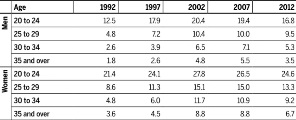
Table 3 shows the distribution of workers, who were students, by sex and age in different years. Naturally, older workers showed smaller pro-portions of individuals studying, as most had already dropped out of the educational system. However, notice the remarkable difference between the sexes. All the proportions for women are much higher than for men, indicating that overall gaps informal education levels are increasing for those already in the labor market.
is natural to expect female empowerment vis-à-vis males in many life di-mensions. This may promote a decrease in the relative differences of time allocation for household chores, implicating a further decrease in labor market gender gaps and a relative increase in females’ investments in work
skills. The final presentation of the descriptive section is on earnings per hour, which complements the preceding discussion.
Table 3 Distribution of workers, who were students, by sex and age in different years
Age 1992 1997 2002 2007 2012
Men 20 to 24 12.5 17.9 20.4 19.4 16.8
25 to 29 4.8 7.2 10.4 10.0 9.5
30 to 34 2.6 3.9 6.5 7.1 5.3
35 and over 1.8 2.6 4.8 5.5 3.5
W
omen
20 to 24 21.4 24.1 27.8 26.5 24.6
25 to 29 8.6 11.3 15.1 15.0 13.3
30 to 34 4.8 6.0 11.7 10.9 9.2
35 and over 3.6 4.5 8.8 8.8 6.7
Source: PNAD 1992, 1997, 2002, 2007 and 2012
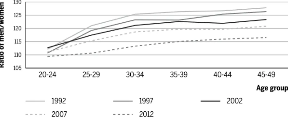
Figure 7 compares hourlywages of men and women at the same schooling level in different years. Men earned more in all schooling levels in all years; however, the gap decreased, especially between 1997 and 2002. Gender gaps increased along with educational level, as suggested by the literature describing glass ceiling effects for income (Albrecht; Bjorklund; Vroman, 2001; Arulampalam; Booth; Bryan, 2007; Rica; Dolado; Llorens, 2008).
Figure 7 Ratio of hourlywages for men and women by educational level in different years
Source: PNAD 1992, 1997, 2002, 2007 and 2012
100 180
160
140
120
0 to 3 4to7 8 to 10 11 12 and over
1992 1997 2002
R
atio men/
w
oman
Schooling level
The next figure presents the gender ratios of hourly wages by age group. First, it demonstrates a remarkable age variation, as younger women are much more similar to their male peers than older ones, in accordance with the idea of growing gender gaps amongearly career professionals (Manning; Swaf-field, 2008). A period variation is also noticed, as ratios decreased between 1992 and 2002. Values between 2002 and 2012 are approximately the same.
Figure 8 Ratio of hourlywages for men and women by age group in different years
Source: PNAD 1992, 1997, 2002, 2007 and 2012
Figure 9 compares the hourlywages of men and women by cohort in diffe-rent years. The numbers show that the ratio between men´s and women´s wages is approximately stable for each cohort, but that younger cohorts show a smaller gap between sexes.
Figure 9 Ratio of hourlywages for men and women by cohort (grouped by age in 1992) in different years
Source: PNAD 1992, 1997, 2002, 2007 and 2012
These two last figures suggested that a cohort effect might exist, as gender wage gaps for younger cohorts are smaller. Figure 8 indicates a variation based on period, but there are confounding factors with cohort and age.
100 160
140
120
25-29 30-34 35-39 40-44 45-49
1992 1997 2002
R
atio men/
w
oman
Age group
2007 2012
105 135
125
115
1992 1997 2002 2007 2012
20-24 25-29 30-34
R
atio men/
w
oman
This section with descriptive statistics clearly indicated that gender gaps in the labor market related to labor market participation, workload, expe-rience and earnings are shrinking; this effect shows most strongly in youn-ger cohorts. Women also have an increasing advantage in educational level.
These five trends put together indicate a convergence between the sexes. We further analyze the data discussed in this section with the use of eco-nometric models in order to better glimpse the convergence between men and women in the labor market. The results are presented in the next section.
6
Results of the econometric models
This section presents the results of the econometric models: first those of the Mincerian models and then those of the hierarchical models.
6.1 Mincerian models
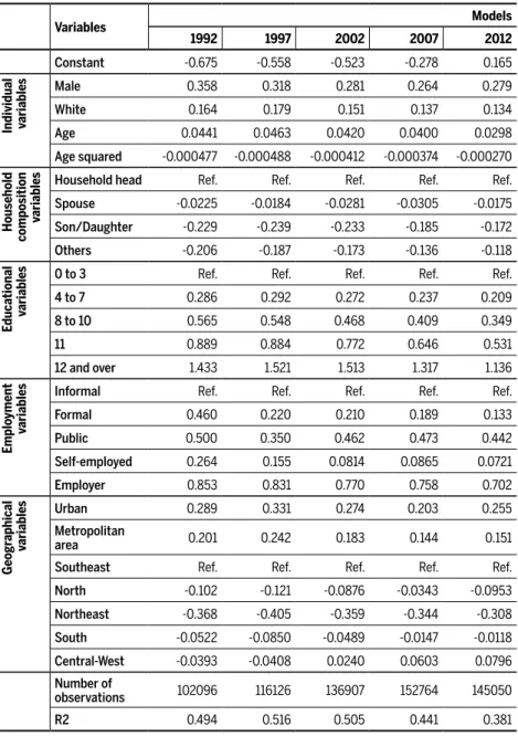
Table 4 shows the results for the Mincerian equations for each year sepa-rately. These models will be the basis for the discussion of all subsequent econometric models. All variables were significant at 5%.
Most results were as expected. White individuals and those who were household heads had higher wages. Notice, however, that the coefficients show a decreasing tendency, suggesting a homogenization in earnings between ethnic groups and between household members.
All coefficients for age were positive and for age squared negative. Due to the dimension of the coefficients, the association of wage and age in all years is increasing for young individuals, assumes a maximum respec-tively at 46, 47, 51, 53 and 55, and decreases afterwards. Notice that the maximum is obtained at higher ages at the end of the period, suggesting an increase in the importance given to labor market experience.
Those who lived in urban and metropolitan areas had higher wages. For
macroregions, the coefficients were mostly negative, as expected, indica-ting that those who lived in the Southeast region had higher wages. The exceptions are the coefficients for the Central-West region, which were negative in 1992 and 1997 and positive afterwards. This indicates that the region was closer to the North and Northeast regions in socioeconomic terms in the beginning of the period, developed at a quicker pace than others, and now resembles the more developed parts of Brazil.
All coefficients for education were positive and increasing in magni-tude with educational level, indicating, not surprisingly, that higher le-vels of education resulted in higher earnings. However, notice that the coefficients for a specific educational level were roughly stable between 1992 and 2002 and diminished after the latter year, suggesting that the premium for education recently decreased in Brazil. Similarly, Trostel, Walker and Woolley (2002) used an OLS model to analyze the trends in returns to education in many countries. They concluded that the returns to schooling did not increase significantly in most countries and decrea-sed in some.
These findings described so far are commonly observed in Mincerian models, and we do not further discuss them. The focus here, however, is study of the male coefficients. In Table 4, they were all positive. That is, after controlling for all the other variables, males had higher hourlywages than females. What about the convergence between the sexes anticipated
in sections 1 and 2?
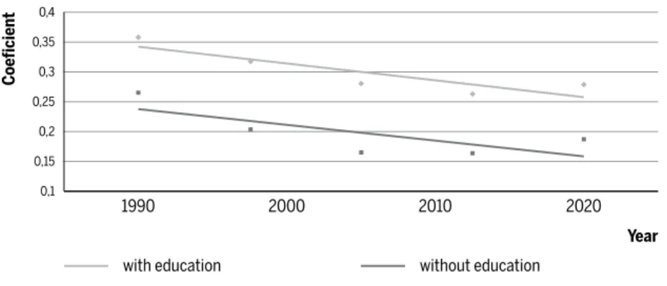
Let´s have a closer look at these coefficients, as shown in Figure 10. This figure plots the values for the five coefficients of the above models, which are around the upper line. Clearly, differences between genders decreased: that is, after controlling for the variables in the model, gender wage gaps decreased; however, they are still quite sizable.
Table 4 Results for the Mincerian models by year
Variables Models
1992 1997 2002 2007 2012
Constant -0.675 -0.558 -0.523 -0.278 0.165
Individual variable
s Male 0.358 0.318 0.281 0.264 0.279
White 0.164 0.179 0.151 0.137 0.134
Age 0.0441 0.0463 0.0420 0.0400 0.0298
Age squared -0.000477 -0.000488 -0.000412 -0.000374 -0.000270
Household
compo
sition
variable
s Household head Ref. Ref. Ref. Ref. Ref.
Spouse -0.0225 -0.0184 -0.0281 -0.0305 -0.0175
Son/Daughter -0.229 -0.239 -0.233 -0.185 -0.172
Others -0.206 -0.187 -0.173 -0.136 -0.118
E
ducational variable
s 0 to 3 Ref. Ref. Ref. Ref. Ref.
4 to 7 0.286 0.292 0.272 0.237 0.209
8 to 10 0.565 0.548 0.468 0.409 0.349
11 0.889 0.884 0.772 0.646 0.531
12 and over 1.433 1.521 1.513 1.317 1.136
E
mplo
yment
variable
s Informal Ref. Ref. Ref. Ref. Ref.
Formal 0.460 0.220 0.210 0.189 0.133
Public 0.500 0.350 0.462 0.473 0.442
Self-employed 0.264 0.155 0.0814 0.0865 0.0721
Employer 0.853 0.831 0.770 0.758 0.702
Geogr
aphical
variable
s Urban 0.289 0.331 0.274 0.203 0.255
Metropolitan
area 0.201 0.242 0.183 0.144 0.151
Southeast Ref. Ref. Ref. Ref. Ref.
North -0.102 -0.121 -0.0876 -0.0343 -0.0953
Northeast -0.368 -0.405 -0.359 -0.344 -0.308
South -0.0522 -0.0850 -0.0489 -0.0147 -0.0118
Central-West -0.0393 -0.0408 0.0240 0.0603 0.0796
Number of
observations 102096 116126 136907 152764 145050
R2 0.494 0.516 0.505 0.441 0.381
Source: PNAD 1992, 1997, 2002, 2007 and 2012 Note: For all coefficients: p <0.05.
op-portunities in a life course perspective, as they had encountered different realities when they started work, and these differences continued to affect them throughout their working lives. Below we show similar Mincerian models with cohorts separated.
Figure 10 Male coefficient in different years with and without control for education
Source: PNAD 1992, 1997, 2002, 2007 and 2012
Due to the increased propensity for retirement of older individuals, we
selected the cohorts for which we have data from all five PNADs, the same cohorts shownin figures 6 and 9. Notice that we are also avoiding the pro-blems of introducing only very young individuals in a particular cohort. It is well known that gender gaps tend to increase when cohorts are in their twenties, and that differences decrease thereafter (Blau; Kahn, 2000).
We focused our attention on the male coefficient, which were all po-sitive and significant, as shown in Figure 11. Similarly to the previous figure, this figure shows the coefficients for the male dummy with and without controlling for educational level, respectively in the upper and lower curve. Notice that the gender gaps for younger cohorts are smaller, suggesting a convergence in wages between the sexes, especially in the analysis which does not control for educational level. Notice, however, that the youngest women we included in the analysis were aged 40 to 44 years old in 2012. That is, they were still negatively affected by the problems faced by women entering the labor market in earlier periods. We did not estimate the coefficients for younger cohorts, as we do not have complete data in all periods, but we expect even smaller gaps in future studies.
0,15 0,3
0,25
0,2 0,35 0,4
0,1
1990 2000 2010 2020
with education without education
Coe
ficient
Figure 11 Male coefficient for different cohorts with and without control for education
Source: PNAD 1992, 1997, 2002, 2007 and 2012
Mincerian models like those used here do have some limitations. For a methodological discussion of how to estimate the returns of education using other methods see Resende and Wyllie (2006), Sachsida, Loureiro and Mendonça (2004), Trostel, Walker and Woolley (2002) and Weich-selbaumer and Winter-Ebmer (2003). Given the objectives of this paper, and in order to partially overcome these limitations, we used hierarchical models based on the APC approach, which are presented below.
5.2 Hierarchical models and the APC approach
This second group of models complements the previously presented Min-cerian models estimated by OLS. We applied different empirical strategies in order to observe the differences between male and female wages from different perspectives. Given the results of the descriptive section and of the previous econometric models, we decided to apply the models for each cohort separately.
Initially, we applied the model presented in the methodological section. Then we relaxed the analysis, dropping some controls, as we had done with the previous models. Again, the objective is to study gender wage gaps from the traditional perspective and then without controlling for edu-cation level and labor market segregation.
Again, the focuses of the analysis are the coefficients for the male dum-my, and we restrict our presentation to them. Table 5 presents the results
0,15 0,3
0,25
0,2 0,35 0,4
0,1
40-44 45-49 50-54
with education without education
Male Coe
ficient
for three different models for the same cohorts already discussed. Moreover, we included two younger cohorts in order to observe very recent labor mar-ket features. Notice that we are not avoiding the problems of introducing only very young individuals in a particular cohort, as we did in the previous models. Gender gaps tend to increase when cohorts are in their twenties, and then differences decrease (Blau; Kahn, 2000). In general, the gender gap for workloads between men and women increased during the workers’ twenties and decreased afterwards, which might explain part of the
diver-gence between sexes in wages for early career (Manning; Swaffield, 2008). Notice that all coefficients in model 1 were positive and significant, indicating that for all cohorts, after controlling for period, individual, employment, geographical and educational variables, that is, a standard analysis, there were significant gender wage gaps in favor of men. Besides, the coefficients were quite similar for all cohorts, indicating stability in the unexplained part of gender wage gaps. It should be emphasized that the results described by this model clearly indicate that men and women in similar occupations received different wages, indicating a persistent unex-plained factor in labor market outcomes which favors men. Besides, as the coefficient was positive for all cohorts, young women are still entering the labor market with lower wages than similar men, but they are expected to catch up at least partially as they age.
The next model drops educational controls. All the coefficients decrea-sed in magnitude, but again all of them were positive, significant and si-milar. From this perspective, overall gender wage gaps are smaller because women are more educated than men are.
Model 3 drops the employment and geographical variables from the controls. The Brazilian labor market is becoming less segregated, and this might enhance females’ wages vis-à-vismales’. Moreover, women tend to be more urbanized than men are. Therefore, if you compare male and female peasants, the former will have higher average earnings. Neverthe-less, if a larger proportion of females migrate to urban areas, wage diffe-rences will possibly growsmaller or even be reversed, as comparisons will be between urban females and rural males. The model shows that the coefficients were non-significant or positive with smaller magnitude. That is, women’s endowments positively influence wages relative to men.
par-tially or totally compensate for this unexplained advantage tomen. Model
1 shows that there are significant unexplained differences between the sexes in the labor market. However, the other models, showing that wo-men have more favorable endowwo-ments and that females are increasingly occupying higher-wage jobs, suggest that in less controlled analysis dif-ferences are smaller or non-significant. However, it should be clear that comparisons are not for similar individuals, as I dropped some controls.
Thus, women are promoting a more dynamic convergence in the labor market because of their endowments, indicating a movement from situa-tion 1 to situasitua-tion 3 in Table 1. Future analysis will tell whether we will move to a time 4 situation. Given that women are becoming more and more present in the labor market and that gaps favoring men are shrin-king, it is not unreasonable to consider such a change probable.
Table 5 Hierarchical models and the APC approach: male coefficient for each cohort
Cohort age in 2012 Model 1 Model 2 Model 3
50 to 54 0.19** 0.16** 0.002
45 to 49 0.20** 0.16** 0.013
40 to 44 0.25** 0.19** 0.064**
35 to 39 0.25** 0.16** 0.047
30 to 34 0.26** 0.17** 0.092**
Controls
Period variables Yes Yes Yes
Individual variables Yes Yes Yes
Employment variables Yes Yes No
Geographical variables Yes Yes No
Educational variables Yes No No
Note: * significant at 10%. ** significant at 5%.
Our final analysis examined the data grouped by cohort and schooling le-vel, as many occupations in the service sector, which has absorbed women better than other sectors relative to men, tend to be occupied by diverse le-vels of educational attainment. The objective is to observe whether gender wage gaps converge differently for different educational levels.
while the second drops the controls for employment type and geography, and hence men and women are not similar in these aspects.
Notice that for levels of education lower than high school, which are
from 0 to 10 years of formal education, the coefficients are mostly positive and significant, indicating gender wage gaps favoring men. Coefficients decreased in magnitude when not controlling for employment and geogra-phy variables; however, they continued to be significant.
Differently, for individuals with a high school diploma or a higher level of education, most coefficients are non-significant, even including all con-trols, suggesting similar wages for both genders for more qualified indivi-duals when the study is done by cohort and educational level. Leone and Baltar (2006) also analyzed gender wage gaps for individuals with higher education in Brazil in the 1990s. They observed that men had greater wa-ges and, as we have, they observed a convergence in values for the diffe-rent sexes.
Based on the glass ceiling literature (Albrecht; Bjorklund; Vroman, 2001; Arulampalam; Booth; Bryan, 2007; Rica; Dolado; Llorens, 2008), this con-vergence between sexes observed for higher educational level might not be observed for income quantiles at the very end of the distribution.
Table 6 Hierarchical models and the APC approach: male coefficient for each cohort and schooling level
Cohort age in 2012
Schooling level
0 to 3 4 to 7 8 to 10 11 12 and above
Controls: Period, individual, employment type and geographical variables
50 to 54 0.17** 0.22** 0.18 0.20 0.38
45 to 49 0.26** 0.18** 0.18* 0.19 -0.01
40 to 44 0.31** 0.29** 0.16* 0.17 -0.042
35 to 39 0.31** 0.24** 0.21** 0.18* 0.013
30 to 34 0.25** 0.33** 0.28** 0.062 0.32
Controls: Period and individual variables
50 to 54 0.041 0.099* 0.070 0.11 0.14
45 to 49 0.10** 0.10** 0.10 0.045 0.12
40 to 44 0.19** 0.20** 0.13* 0.086 -0.058
35 to 39 0.19** 0.17** 0.16** 0.13 -0.00
30 to 34 0.21** 0.25** 0.28** 0.089 0.33
We end this section by answering the question of whether or not there are a considerable convergence between the sexes in the Brazilian labor market. If we return to Table 1, considering the results of these last two tables, the answer is partially yes. Surely, the Brazilian labor market is evolving from situation 1 to situation 2 and, in some aspects, to situation 3. We observed that women generally possess better endowments for the labor market; ho-wever, although differences are shrinking, a sizable proportion of the wage gaps continues to be unexplained, possibly due to discrimination.
7
Final commentaries
The main objective of this paper was to discuss gender wage gaps in the Brazilian labor market using an APC approach. Historically, men have do-minated the labor market, as males’ participation was greater and gender wage gaps favored men. However, some recent trends might change this perspective, as the labor market is increasingly becoming a women’s locus and in many aspects females in Brazil nowadays have better endowments for the labor market than men. Indeed, the empirical analysis showed a convergence in the Brazilian labor market, especially when gender wage gaps and labor market segregation are analyzed conjointly.
This paper described labor market trends between 1992 and 2012 using PNADs. The descriptive section clearly indicated that gaps in the labor market, such as labor market participation, workloads, experience and earnings, are shrinking between sexes. The gap in educational level is in-creasing, but this gap favors females. These five trends put together clearly indicate a convergence in the Brazilian labor market.
We further analyzed the data with Mincerian wage equations estimated by OLS for different years, and observed a slight tendency toward wage convergence by gender, especially without controls for educational level. Moreover, we also analyzed models by cohort; the results of this analysis were more striking, indicating smaller differences for younger cohorts and a clearer tendency toward convergence.
educa-tional attainment, women´s endowments for the labor market are better than men´s, and partially compensate the unexplained differences. Mo-reover, differences in earning between sexes for individuals with at least a high school diploma, when controlling for cohort, were non-significant, indicating a gender wage convergence for more qualified people.
This general tendency toward convergence between genders might be even more pronounced if we take into account that a greater negative selection is expected on males’ labor market dropout in Brazil vis-à-vis females, as is observed in the U.S. For instance, in the U.S., black males who were high school dropouts decreased their labor market participation from 91% to 59% between 1969 and 2004, a much greater decrease than in other population groups. Moreover, this decline may be even underesti-mated, as many low-qualified black males in the U.S. were in institutions and did not enter the labor market statistics (Juhn; Potter, 2006). In Brazil, many young unqualified males are becoming part of the triple no group: they do not study, do not work and do not look for a job (Camarano; Kan-so, 2008). Hence, they do not enter the Brazilian labor market statistics, except for participation.
The labor market dynamics shown in this paper strongly suggests that the Brazilian labor market evolved to a more homogenous situation between the sexes, although still with considerable gaps between men and women. Future analysis will show if Brazil will one day have a homo-genous labor market regarding the sexes. Given the growing educational gaps between the sexes in favor of women, and given that unexplained differences in the labor market, including discrimination, tend to decrease as social roles and norms evolve, our educated guess is that this trend is quite probable.
References
AMATO, P.; ROGERS, S. Do attitudes toward divorce affect marital quality?Journal of Fami-lies Issues, v. 20, n. 1, p. 69-86, 1999.
ALBRECHT, J.; BJORKLUND, A.; VROMAN, S. Is there a glass ceiling in Sweden?IZA DP No. 282, 2001.
ARABSHEIBANI, G.; CARNEIRO, F.; HENLEY, A. Gender wage differentials in Brazil: trends over a turbulent era. World Bank policy research working paper, n. 3148, 2003.
Explo-ring the gender pay gap across the wage distribution. Industrial and Labor Relations Review, v. 60, n. 2, 2007.
BAILEY, M.; HERSHBEIN, B.; MILLER, A. The opt-in revolution? Contraception and the gender gap in wages. NBER working paper series, n. 17922, 2012.
BARROS, R.; CORSEUIL, C.; SANTOS, D.; FIRPO, S. Inserção no mercado de trabalho: di-ferenças por sexo e consequências sobre bem-estar. Texto para discussão n. 796, Rio de Janeiro: IPEA, 2001.
BLAU, F.; KAHN, L. Gender differences in pay. NBER working paper, n. 7732, 2000.
BROWN, C.; CORCORAN, M. Sex-based differences in school content and the male/female wage gap. NBER working paper, n. 5580, 1996.
BRUSCHINI, C. Trabalho doméstico: inatividade econômica ou trabalho não-remunerado? Revista Brasileira de Estudos Populacionais, v.23, n.2,p.331-353, 2006.
CAMARANO, A.; KANSO, S. O que estão fazendo os jovens que não estudam, não traba-lham e não procuram trabalho? Boletin Mercado de trabalho: conjuntura e análise. Brasília: IPEA, n. 53, p. 37-44 (nota técnica), 2008.
CAMARGO, J.; SERRANO, F. Os dois mercados: homens e mulheres na indústria brasileira. Revista Brasileira de Economia, n.34, 1983.
FERNÁNDEZ, R.; WONG, J. The disappearing gender gap: the impact of divorce, wages, and preferences on education choices and women’s work. NBER working paper series, n. 17508, 2011.
GARCÍA, J.; HERNÁNDEZ, P.; LÓPEZ-NICOLÁS, A. How wide is the gap? An investigation of gender wage differences using quantile regression. Empirical Economics, v.26, p.149-167, 2001.
GLOMM, G.; JUNG, J.; TRAN, C. Macroeconomic implications of early retirement in the public sector: The case of Brazil. Journal of Economic Dynamics & Control, v.33, p.777–797, 2009.
GOLGHER, A. Diálogos com o ensino médio 3: O estudante jovem no Brasil e a inserção no mercado de trabalho. Working paper, Cedeplar, nº 393, 2010.
HECKMAN, J.; LOCHNER, L.; TODD, P. Fifty years of Mincer earnings regressions. NBER, Working Paper 9732. Cambridge:2003.
JENSEN, R. Do labor market opportunities affect young women’s work and family deci-sions? Experimental evidence from India. The Quarterly Journal of Economics, v.127, p. 753-792, 2012.
JUHN, C.; POTTER, S. Changes in Labor Force Participation in the United States. Journal of Economic Perspectives. v.20, n.3, Summer, p.27-46, 2006.
KHAMIS, M. Comparative advantage, segmentation and informal earnings: a marginal treat-ment effects approach. IZA discussion paper, n. 3916, 2008.
LEME, M.; WAJNMAN, S. Tendências de coorte nos diferenciais de rendimentos por sexo. In: HENRIQUES, R. (Org.). Desigualdade e pobreza no Brasil. Rio de Janeiro: IPEA, 2000. LEONE, E.; BALTAR, P.Diferenças de rendimento do trabalho de homens e mulheres com
MADALOZZO, R. Occupational segregation and the gender gap in Brazil: an empirical analysis. Economia Aplicada, v.14, n.2, p.147-168, 2010.
MANNING, A.; SWAFFIELD, J. The gender gap in early-career wage growth. The Economic Journal, v.118 (July), p.983–1024, 2008.
MASON, W.; SMITH H. Age-Period-Cohort Analysis and the Study of Deaths from Pulmo-nary Tuberculosis. In: MASON, W.; FIENBERG, S. (Ed.) Cohort Analysis in Social Research. New York: Springer-Verlag, p.151-228, 1985.
MAUME, D.; SEBASTIAN, R. Gender, nonstandard work schedules, and marital quality. Jour-nal of Family and Economic Issues, v.33, p.477–490, 2012.
MIKI, M.; YUVAL, F. Using education to reduce the wage gap between men and women. The Journal of Socio-Economics, v.40, p.412-416, 2011.
MONTALI, L. Relação família-trabalho: reestruturação produtiva e desemprego. São Paulo Perspec., v.17 n.2, 2003.
ÑOPO, H. Promoting equality in the country with the largest earnings gaps in the region: Brazil 1996-2006. In:New Century, Old Disparities: Gender and ethnic earnings gaps in Latin America and the Caribbean. Washington D.C.: Inter-American Development Bank and World Bank, 2012a.
ÑOPO, H.More schooling, lower earnings: women´s earnings in Latina America and the Caribbean. In:New Century, Old Disparities: Gender and Ethnic Earnings Gaps in Latin America and the Caribbean. Washington D.C.: Inter-American Development Bank and World Bank, 2012b.
POTTER, J.; SCHMERTMANN, C.; ASSUNÇÃO, R.; CAVENAGHI, S. Mapping the Timing, Pace, and Scale of the Fertility Transition in Brazil. Population and Development Review, v. 36, n. 2, p. 283-307, 2010.
OLIVEIRA, A. A segregação ocupacional por sexo no Brasil. 1997. Dissertação (Mestrado em
Demografia) - Cedeplar, UFMG, Belo Horizonte, 1997.
QUEIROZ, B. The evolution of retirement in Brazil. In: XV Encontro Nacional de Estudos Popu-lacionais, ABEP, Caxambu – MG, Brazil, 2006.
RESENDE, M.; WYLLIE, R. Retornos para e educação no Brasil: evidências empíricas adicio-nais. Economia Aplicada, v. 10, n. 3, p. 349-365, 2006.
RICA, S.; DOLADO, J.; LLORENS, V. Ceilings or floors? Gender wage gaps by education in
Spain. Journal of Population Economics, v.21, p.751-776, 2008.
RYDER, N. The cohort as a concept in the study of social change. American Sociological Review, v.30, n. 6, p.843-861, 1965.
SACHSIDA, A.; LOUREIRO, P.; MENDONÇA, M. Um estudo sobre retorno em escolaridade no Brasil. Revista Brasileira de Economia, v. 58, n. 2, p. 240-265, 2004.
SALARDI, P. The evolution of gender and racial occupational segregation across formal and non-formal labor markets in Brazil, 1987 to 2006. Review of Income and Wealth, 2014. SILVA, D.; CARVALHO, A.; NERI, M. Diferenciais de salários por raça e gênero no Brasil:
Aplicação dos procedimentos de Oaxaca e Heckman em Pesquisas Amostrais Complexas.