Tiago Cavalcanti
†
, Márcio Corrêa
‡
Contents: 1. Introduction; 2. The Model; 3. Equilibrium and Analytical Results; 4. Quantitative Exercises; 5. Concluding Remarks; A. Proof of Proposition 2.1; B. Proof of Proposition 3.1.
Keywords: Income Transfers, Job Creation, Job Destruction.
JEL Code: D83, E24, J20.
This paper studies the effects of cash transfers to the poor on the labor market. We build a matching model of the labor market with endogenous job destruction in which agents can be in three states: employed, unemployed, or out of the labor force (home production). Workers are heterogenous in their labor market productivity. An idi-osyncratic productivity shock arrives at constant instantaneous rate. Depending on this shock, workers might want to leave the labor mar-ket and workers out of the labor force might decide to look for a job. We introduce cash transfers to all agents with income below some th-reshold level. Our analytical results show: (i) The size of cash transfers has a negative effect on the employment rate, but an ambiguous effect on the unemployment rate; and (ii) the coverage of this welfare pro-gram has a positive effect on the employment rate, and an ambiguous effect on the unemployment rate. We also provide some numerical si-mulations.
O presente artigo estuda os efeitos das políticas de transferência de renda para a população de baixo poder aquisitivo sobre o mercado de tra-balho. Para tal, foi desenvolvido um modelo de busca de emprego com de-struição endógena, em que os agentes podem estar em três situações distin-tas: empregado, desempregado ou fora da força de trabalho, neste caso, en-volvidos na produção de um bem doméstico. No presente modelo considera-se que os trabalhadores são heterogêneos em sua produtividade no mercado de trabalho e que há um choque de produtividade idiossincrático que chega a uma taxa instantânea constante. Dependendo da dimensão deste choque, os trabalhadores podem decidir abandonar o mercado de trabalho enquanto outros fora da força de trabalho podem decidir buscar emprego. O programa
∗We thank, without implicating, Carlos Eugênio da Costa and audience at CAEN-EPGE meeting for comments. †University of Cambridge. E-mail:[email protected]
de transferência de renda considerado no modelo tem como beneficiários to-dos os agentes com renda abaixo de um determinado nível. Dentre os re-sultados obtidos, verifica-se que: (i) a dimensão da renda transferida tem efeito negativo sobre a taxa de emprego e um efeito ambíguo sobre a taxa de desemprego; (ii) a cobertura do programa de transferência de renda tem efeito positivo sobre a taxa de emprego e efeito ambíguo sobre a taxa de de-semprego. Para dar maior consistência aos resultados apresentados foram realizados alguns procedimentos numéricos.
1. INTRODUCTION
In his study about the growth of social spending in the last three centuries, Peter Lindert posits that: “The first kind of social spending to exceed 1 percent of national product was, and still is, the most controversial kind: direct assistance to the poor”(Lindert, 2004, p. 39). Some of these assistance to the poor are in kind, but there are also transfers in cash.1Recently, many developing countries have adopted some type of conditional cash transfers to the poor as a mechanism to fight poverty, malnutrition, and inequality. Two examples are theBolsa Famíliain Brazil andProgressain Mexico, but similar programs are widespread around the world, including one in the city of New York (see Currie and Gahvari, 2008). UnderBolsa Família, for instance, families with income less than R$ 60 (roughly US$ 38) per capita receive R$ 62, plus R$ 20 per child (aged 15 and lower) up to three children, and R$ 30 per adolescent (aged 16 and 17) up to two children. Therefore, poor families can receive up to R$ 182, which is about half of a minimum wage in Brazil. The conditionalities of these transfers are the beneficiary families compliance with requirements such as school attendance, vaccine, and pre-natal visits (see Brazilian Ministry of Social Development). The total coverage is large: Roughly 11.1 million families or about 44 million people. In the poorest Brazilian region, i.e., in the Brazilian Northeast about 49 percent of all families is enrolled in this program.2
In this paper we study the effects of such cash transfers program on the labor market:3 What are the effects of cash transfers to the poor on the unemployment rate, employment rate, and participation rate? What are the effects on inequality and productivity? In order to address these questions, we build a matching model of the labor market based on Diamond (1982), Mortensen (1982), and Pissarides (1990) where workers can be in three states: employed, unemployed, or out of the labor force, producing the consumption good at home.4The model is based on a recent contribution by Garibaldi and Wasmer (2005). There is a matching technology, which makes the number of successful matches at any moment
1In his bookCapitalism and Freedom, Milton Friedman (1962) also advocates cash transfers to the poor as a social measure to
alleviate poverty.
2In some very poor cities, such as Manari in the state of Pernambuco, 90 percent of all families participates in the program.
Estimates show that government spending on this program accounts by only 0.3 percent of total GDP. Soares et al. (2006), for instance, show that this cash transfer program is well targeted and it accounts for 28 percent of the fall in the Gini inequality index between 1995 and 2004 and corresponds to about 0.82 percent of the total family income reported at the Brazilian National Household Survey (PNAD). For comparison, they show that pensions equal to the minimum wage account for 32 percent to the fall in the Gini inequality index in the same period, but they make up to 4.5 percent of the total family income. Therefore, theBolsa Famíliaseems an effective way to fight inequality and poverty.
3Most of the time the goals of these programs are to: (i) reduce poverty and inequality; and (ii) break the inter-generational
transmission of poverty by conditioning these transfers on beneficiary compliance with, for instance, school attendance. It is not our goal in this paper to investigate the long run effects of such cash transfer, but instead to study its impact on the labor market.
4Search and matching models are the main tools used in macroeconomics to evaluate the effects of policies on the labor market.
in time a function of the aggregate measures of unemployed workers and vacant jobs. As in Mortensen and Pissarides (1994), job destruction is endogenous. Workers are heterogenous in their labor market productivity. A new productivity level arrives at constant instantaneous rate. Depending on the shock of their productivity level, workers might want to leave their job and workers out of the labor force might decide to search for a job.
We introduce cash transfers to the poor in this framework. The government provides benefits, b > 0, to all workers with income less thanw. It is important to highlight that differently from un-employment insurance, workers in this welfare program receive cash transfers independently whether they are working, unemployed, or out of the labor force – working in home production. The only re-quirement to be entitled to this program is to have income less thanw.5 We investigate the effects of the size and the coverage of cash transfers on the labor market. We show the following qualitative results:
(i) the size of cash transfers has a negative effect on the employment rate, but an ambiguous effect on the unemployment rate. Participation rate is affected negatively; and
(ii) the coverage of the program has a positive effect on the employment rate, and an ambiguous effect on the unemployment rate.
We also provide some numerical simulations, which allow us to investigate the effects of cash transfers on income inequality, and analyze alternative polices. From our knowledge, we were the first to analyze the impact of cash transfers on the labor market in a matching model with endogenous job destruction and labor market participation.
Besides this introduction, this paper has three more sections: In Section 2 we develop the matching model with cash transfer and labor market participation. Section 3 defines the equilibrium and pro-vides some analytical results. Section 4 propro-vides some numerical simulations. Section 5 contains the concluding remarks.
2. THE MODEL
2.1. Set up
Time is continuous and there are two commodities in this economy: one consumption good and one labor input. The economy is inhabited by a continuum of infinitely lived agents of measure one who are heterogenous with respect to their labor market productivity,x. There is also a continuum of measure one of firms. Each firm has access to a production technology that exhibits constant returns to scale with labor as the only input. Without loss of generality, we assume that each firm employs at most one worker. When employed, a worker producesyxunits of the consumption good. Both workers and firms are neutral to risks and discount the future at a constant exogenous rater.
As in Garibaldi and Wasmer (2005), workers can be in three states: Employed and receiving the market wagew(x)in units of the consumption good; unemployed and searching for a job; or working at home producinghunits of the consumption good.6Worker’s productivity in the market is stochastic and is determined by a general distributionG(x), with support in the unit interval. Productivity x changes over time according to a Poisson process with arrival rateψ. In this way, workers productivity
and Sargent (1998), Pavoni and Violante (2007), among others. For the effects of firing costs, see, for instance, Blanchard and Portugal (2001), Bertola and Rogerson (1997), Cavalcanti (2004), and Ljungqvist (2002).
5This article is part of a project (Cavalcanti and Corrêa, 2009), in which we investigate the effects of different welfare programs
on the labor market.
6We could also have assumed that agents searching for a job can also produceshwiths∈(0,1)in home production. Such
can move, with probabilityψto a new productivity value that can be bigger or lower then the previous value.7Note that workers productivity can be hit by a shock moving workers to a situation of program coverage. Before starting a productive activity, workers and firms are involved in a search process for a productive partner, wherecequals search cost for the firm. The number of job matches formed per period is given by a non-negative, concave and homogeneous of degree one function,m(v,u), which is crescent in its two arguments, wherevequals vacancy rate andudenotes the fraction of unemployed workers. By the homogeneity assumption, we can write the probability rate of filling a vacancy as: q(θ) =m(u,vv )=m(1θ,1), whereθ= v
udenotes the tightness of the labor market. In addition, the rate
at which an unemployed worker moves to employment isθq(θ) =m(uu,v).
2.2. Government sector
There is a government that provides income transfers,b >0, to all workers with income less than w. Workers receive income transfers independently whether they are working, unemployed, or out of the labor force, i.e., working in home production. As in Acemoglu et al. (2001), we assume that cash transfers are financed through lump-sum taxes.
2.3. Workers
LetWN B(x)andWB(x)be the asset value for a worker with productivityxof being employed receiving or not benefits, respectively. LetU(x)be the asset value of being unemployed. The following Bellman equations describe the problem of a worker with productivityx:
(r+ψ)WN B(x) = w(x) +ψ
Z M
0
max{WB(z),U(z)}dG(z) (1)
+ ψ
Z 1
M
max{WN B(z),U(z)}dG(z)
(r+ψ)WB(x) = w(x) +b+ψ
Z M
0
max{WB(z),U(z)}dG(z) (2)
+ ψ
Z 1
M
max{WN B(z),U(z)}dG(z)
(r+ψ)U(x) = b+ max{h,θq(θ)G(M)[WB(x)−U(x)] (3)
+ θq(θ)(1−G(M))[WN B(x)−U(x)]}+ψ
Z 1
0
U(z)dG(z)
Equation (1) implies that employed workers without government benefits receivew(x)flow units of the consumption good in wages, and at instantaneous rateψobtain a new value for their produc-tivity, which may lead them to leave the job. Equation (2) is analogous to Equation (1). It implies that
7Observe that our productivity process implies that conditional on the arrival of a shock, workers’ new productivity is
employed workers with income less thanwreceive flow incomew(x)plus benefitsb, and at rateψ obtain a new value for their productivity, which might lead them to change their employment status. Observe thatM =w−1(w)corresponds to the productivity level such that ifx < Mworkers receives cash transferb, and ifx > M, workers do not receive government benefits.8Equation (3) suggests that workers without a job receiveband they might choose between home activities receivinghfrom home production or they might choose to search for a job.9At rateψ, workers draw a new productivity level, x, revaluating their choice between seeking for a job or remaining in home production. Notice that once a job match is formed, it can only be destroyed endogenously, due to variations related to market productivity.
2.4. Firms
LetV andJ(x)describes the asset values for a firm of a vacant and a filled job with a worker with productivityx, respectively. They are described by the following Bellman equations:
rV = −c+q(θ)[Je(x)−V] (4)
(r+ψ)J(x) = yx−w(x) +ψ
Z 1
0
max{J(z),V}dG(z) (5) A firm with a vacant position spends flowcin searching for a worker and at rateq(θ)the firm fills this vacancy. Observe that, before a position is filled firms do not know the productivity of the worker or the quality of the match.Je(x)therefore represents the expected value of filling a vacant position. In addition, a firm with a filled job produces flowyxof the consumption good, payingw(x)in wage. At rateψ, the worker that fills this vacancy obtains a new productivity level, which allows the firm to reevaluate their decision to continue producing with this worker or destroy the match to search for a new one.
Free entry in the labor market implies that no economic rents can be gained from vacancy, i.e., V = 0. Therefore, from (4) we have that:
Je(x) = c
q(θ) (6)
There is job creation up to the point where the expected value of a new job match equalizes the cost of occupying a vacancy, expressed in terms of the rate that this position becomes occupied.
2.5. Reservation productivities
Once a job match is formed, there is an economic surplus that must be divided between the worker and the firm. As standard in the literature, we assume that this surplus is divided according to the Generalized Nash Bargaining between firms and workers:
β[J(x)−V] = (1−β)[Wj(x)−U(x)], j=N B, B (7) whereβdenotes workers’ bargaining power.
8As we will show, wages are a function of the labor market productivity.
9Alternatively, we could have added a Bellman equation for being out of the labor force, such that:
H=h+b+ψ
Z 1
0
max{H(z), U(z)}dG(z).
It is important to define the reservation productivity that makes workers indifferent between work-ing in the market or in home production,E, and also the productivity level that makes workers indif-ferent between searching for a job or working at home,R. The surplus generated by a match is:
Sj(x) =J(x) +Wj(x)−U(x), j =N B, B (8) Using equations (1), (2), (3) and (5), evaluatingSj(x)forj=N BandBatx=E, and subtracting
Sj(E)fromSj(x), we have that:
βSj(x) = βy(x−E
j)
r+ψ , j=N B, B (9)
The surplus for both cases have the same structure becausebaffects uniformly the outside option of all workers.
Equation (3) implies that when workers are indifferent between searching for a job or engaging in home activities, then:
h
θq(θ) =βy(
Rj−Ej
r+ψ ), j =N B, B (10)
The left hand side of (10) represents workers’ expected opportunity search cost. The right hand side stands for the benefits obtained with market participation. Sinceh >0, then the left hand side of (10) is always positive, andRj > Ej. Moreover, since the left hand side of (10) is the same whether the worker receive or not benefits, thenRN B−EN B=RB−EB.
Following Garibaldi and Wasmer (2005), the market exit dynamics is determined by:
EN B = b+h+
ψy r+ψ
R1
EN BG(x)dx
y (11)
EB = h+
ψy r+ψ
R1
EBG(x)dx
y (12)
Proposition2.1. Ifb >0, thenEN B> EBandRN B> RB.
Proof:See Appendix A.
Expressions (11) and (12) determine the level of productivity resulting from indifference between working in the market or engaging in home activities. The left hand side of both equations gives the level of productivity that makes workers indifferent between leaving or not the job to home production. The right hand side represents the gain obtained by being employed. Observe that the higher income transfers,b, the higher will be the exit rate, since the value of being at home increases. However, the levels of reservation productivity(Ej,Rj)
j=N B,Bdo not depend on productivity levelM =w−1(w)
and some of these threshold values might not be binding depending on the coverage of the program. In an economy without the cash transfer program (e.g.,M =w−1(w) = 0), workers without a job and with productivity in the interval(EN B,RN B)are marginally attached to the labor market. If they had
a job, they would be working in the labor market, but they are not willing to pay the searching cost (see Garibaldi and Wasmer (2005) and Jones and Riddell (1999)). Employed workers with productivity in this interval at some point in time had productivity aboveRN Bbut if they loose their job they will
2.6. Job creation
Using equations (6) and (9) yields:
Je(x) = (1−β)S(x) = c
q(θ) =
(1−β)y(Rj−Ej)
r+ψ (13)
which determines the dynamics for new job creation. The right hand side of (13) describes the firm benefit of filling a vacant position. The left hand side represents the expected cost related to filling this vacancy. The larger the difference(Rj−Ej), the higher will beθ, thus the higher will be the new job
creation dynamics.
2.7. Wage determination
Using equations (1)-(7), we obtain four wage functions. Firstly, ifx > M, then:
wN B1 (x) = βyx+ (1−β)(b+h), forx < RN B (14) wN B2 (x) = β(yx+cθ) + (1−β)b, forx > RN B (15) Moreover, ifx < M, then:
wB1(x) = βyx+ (1−β)h,forx < RB (16) wB2(x) = β(yx+cθ), forx > RB (17) Observe that the four previous equations give us the wage rates considering that once unemployed, the worker either migrates to home production or returns to the labor market to look for a new job opportunity. The wage rates are composed by two terms: one related to workers’ job match productivity and the other to workers’ outside option. The outside option varies whether workers receive or not benefits and whether his productivity is larger than reservation productivity Rj,j = N B, B. It is
important to observe that some of these wages might not be binding, depending on the productivity levelM associated with incomew.Recall that all workers with productivityx < EBwill be out of the labor force.
Five cases are possible and we study them below:
Case 1: IfM =w−1(w)< EB, then only unemployed workers and those out of the labor force will
receive government income transferb. In this case, equations (16) and (17) will not be binding. Workers with productivityx < EN Bwill be out of the labor force. Marginally attached workers are those with
productivity in the interval[EN B,RN B].
Case 2: IfEB < M = w−1(w) < RB, then only workers unemployed, out of the labor force and
those with productivityx ∈ [EB,M)will receive government benefits. Equation (17) will not bind.
Interestingly, agents with productivityx ∈ [M, EN B]will be out of the labor force, despite the fact
that workers with lower productivity,x∈[EB,M), might be working in the market. This is because if
workers with productivityx∈[M, EN B]have a job, they will not receive cash transfers. The measure
of marginally attached workers is given by:x∈[EB, M]S[EN B,RN B].
Case 3:IfRB < M =w−1(w)< EN B, then all equations will bind. Similarly to Case 2, agents with
productivityx∈[0,EB]S[M, EN B]will be out of the labor force. The measure of marginally attached
Case 4:IfEN B< M =w−1(w)< RN B, then all equations will bind. Only workers with productivity
less thanEBwill be out of the labor force. Marginally attached workers are those with productivityx
in the interval[EB,min{M,RB}]S[M,RN B].
Case 5:IfRN B< M =w−1(w), then all equations will bind, except Equation (14). Agents out of the labor force are those with productivity less thanEB. The measure of marginally attached workers is
given by:x∈[EB, RB].
Notice that Case 1 does not have any effect on the labor market, since there will be no employed worker receiving benefit. Cash transfers will, however, have distributional and welfare effects. Cases 4 and 5 are those in which most of the workers receive cash transfers. Cases 2 and 3, in our point of view, are the two most interesting ones. In these two cases, some workers will decide to leave the labor force (if they work, they will not receive benefits), despite the fact that some workers with lower productivity are actively working in the market.
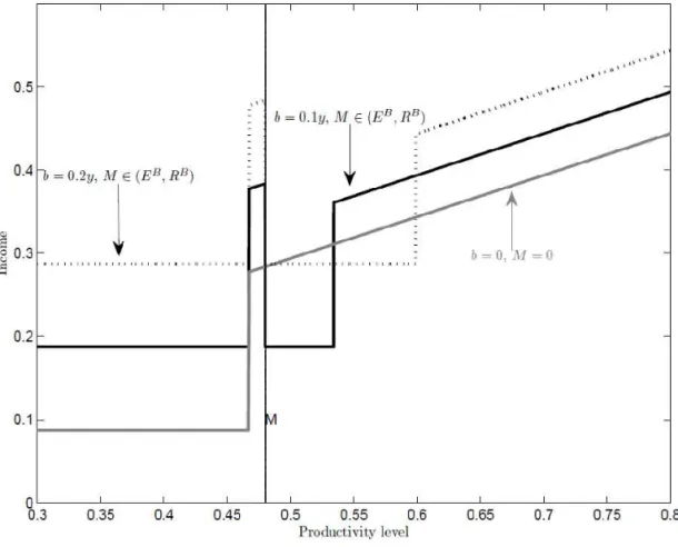
Figure 1 displays the effects of cash transfers on income for different levels of productivity. The grey solid line corresponds to the income of each household, who are heterogeneous in the labor market productivity, in the case without the cash transfer program. Notice that there is a threshold value of productivity, such that if agents’ productivity is below this level, they prefer to stay out of the labor force. When we introduce the cash transfer program10 (black solid line) labor market participation decreases, and some workers with productivity betweenM andEN Bdecide to leave the labor force.
They choose to do so because they will loose benefits in case they find a job. There are, however, workers with lower productivity that are actively working in the labor market. Notice that as we increase the size of transfers further (black dotted line), labor market participation decreases more.
3. EQUILIBRIUM AND ANALYTICAL RESULTS
The equations that describe employment and unemployment dynamics are given by:
˙
e = [θq(θ)u−ψG(EB)e]G(M) + [θq(θ)u−ψG(EN B)e][1−G(M)] (18)
˙
u = {−[θq(θ) +ψG(RB)]u+ψ[1−G(RB)](1−e−u)}G(M) +... (19)
{−[θq(θ) +ψG(RN B)]u+ψ[1−G(RN B)](1−e−u)}[1−G(M)]
Notice that in both equations we separate the flow of workers that receive or not benefits. In the employment equation, there are two flows: the first one represents the rate at which unemployed workers migrate to employment (θq(θ)u), while the second one equals the rate in which workers move from employment to home production (−ψG(Ej)e). In the unemployment equation there are three flows: the flow of unemployed workers who find a job in the market (−θq(θ)u); the flow of unemployed workers who move to home production (−ψG(Rj)u); and the flow of agents who move from home
production to unemployment (ψ[1−G(Rj)](1−e−u)).
In the steady-statee˙= ˙u= 0and therefore:
e = θq(θ)u
ψ{G(EB)G(M) +G(EN B)[1−G(M)]} (20)
u = (1−e)ψ{[1−G(R
B)]G(M) + [1−G(RN B)][1−G(M)]}
θq(θ) +ψ (21)
10This is the case in whichEB
Figure 1: The effects of cash transfers on income. Grey solid line: case without cash transfer. Black solid line: case with cash transferb= 0.1yandM ∈(EB,RB). Black dotted line: case with cash transfer b= 0.2yandM ∈(EB,RB)
Now, we can define the equilibrium for this economy.
Definition:Given government policies(b, w), a steady-state equilibrium for this economy is a seven-tuple:
(θ, Rj, Ej, wj
1(x), w
j
2(x), u, e)j=N B,Bsuch that equations (14)-(17), (10)-(13), (20) and (21) are satisfied.
The equilibrium has a block recursive structure. From equations (11) and (12), we can findEN Band
EB. Using equations (10) and (13) we obtain:
θ=(1−β)h
βc .
GivenθandEj, we can use (10) to findRj.
The following proposition establishes the analytical effects of government policies(b, M =w−1(w)) on the steady-state level of employment and unemployment.
Proposition3.1. Consider a steady-state equilibrium. Then, for given government policies(b, M=w−1(w))>>
0, we have that:
i. baffectsenegatively; andbaffectsuambiguously;
ii. Maffectsenon-negatively; andMaffectsuambiguously.
Proof:See Appendix B.
When cash transfer,b, increases there are two opposing effects on unemployment: First, for relative high productive workers (i.e., workers with productivity level higher thanRN B) the opportunity cost
of searching increases – because if they get a job they will loose benefits, therefore some of them choose to leave the labor market, which decreases unemployment. However, for less productive workers (i.e., with productivity slightly higher thanEN B) the opportunity cost of being employed increases, and
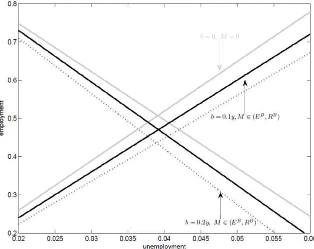
some of them choose to leave their job to home production. This decreases employment (and the labor force) and consequently increases the unemployment rate. Figure 2 illustrates the effects of cash transferbon the unemployment and employment rates. It shows that while the unemployment rate is almost unchanged, the employment rate decreases as the level of benefits increases.
The productivity levelsEi and Ri for i = BandN B are independent of the coverage of the program M. When the coverage of the program increases then there might be an increase in the fraction of workers that might work only because they receive benefitsx∈ [EB,min{M, RB}]. See
this also in Figure 1, which is the interval between the productivity in which workers are indifferent between working in the market or at home and the productivity in which workers become eligible to the program. This would increase the number of employed workers without increasing the number of workers searching for a job. In this case, the employment rate increases and the unemployment rate might decrease. However, ifM increases further such thatM > RB, then there might be some
workersx ∈[RB,M]that might look for a job only because if they find one they would still receive
benefits. The unemployment rate will increase.
4. QUANTITATIVE EXERCISES
4.1. Calibration
In order to quantitatively investigate the main results derived previously, we solve the model numer-ically. We choose a model economy without government benefits, i.e.,b= 0. We first have to calibrate the parameter values such that they are consistent to the empirical observations in the United States. We assume that distributionG(x)is uniform with support in the unit interval. We normalize output y to one. We let the model period be a month and set the discount rater = 0.0033, making the an-nual interest rate equal to 4 percent. Following Ljungqvist (2002), we let the matching technology be represented by a Cobb-Douglas type function:
m=m(u,v) =uαv1−α, with α∈(0,1) (22)
We assume the same elasticity of the matching technology with respect to each input, i.e.,α= 0.5, which was a number estimated by Blanchard and Diamond (1989). We let the worker’s surplus shareβ to be equal to 0.5, which is also used in the matching literature.
Figure 2: The effects of cash transfers on the employment and unemployment rate
rate is equal to 3.5 percent, the tightness of the labor market is equal to 0.5, and the extended unem-ployment rate11is 40 percent larger than the conventional measure (see Garibaldi and Wasmer (2005)). We found the following values for these three parameters:c= 0.175y,h= 0.5c, andψ= 0.11.
Table 1 lists the value of each parameter and includes a comment on how each was selected.
4.2. Simulations
The first row of Table 2 displays for the calibrated economy (b = 0andM = w−1(w) = 0) the unemployment rate, extended unemployment rate, the employment rate, and the income Gini index.12 Then, we introduce a cash transfer program in this economy. For the case thatb= 0.1yandM = 0.47
(i.e.,M ∈ (EB,RB)), cash transfers correspond to roughly one fifth of the average wage. Observe
11This is the unemployed rate plus the rate of marginally attached employed workers.
12The Gini index measures the level of income inequality. Income in this case corresponds to the labor income of those that are
Table 1: Parameter values, baseline economy.
Parameters Values Comment/Observations
y 1 Value normalized to one
r 0.0033 Discount rate: annual interest rate of 4%
β 0.5 Worker’s bargaining power
α 0.5 Parameter of the matching technology
c 0.175 Search cost: calibrated to matchθ= 0.5
h 0.0875 Home production: calibrated to matchu= 3.5
ψ 0.11 Calibrated to match extended unemployment rate,u+ema
=4.9%
that as the size of the income transfers increases, employment decreases and unemployment remains roughly constant (see also Figure 2), though our extended unemployment rate measure, which includes the marginally attached employed workers, increases substantially. It increases by 24 percent. Partici-pation rate also decreases and income inequality decreases sharply. Notice that when we increase the coverage of the program, keeping the size of the transfer constant, both employment and participation rate increase. The program seems to have a negligible impact on government finances. Total spending as a share of output13in the economy withb= 0.1andM = 0.47is about 0.01 percent.
Table 2: Quantitative effects: Cash Transfers
Unemployment Extended Employment Income rate,u Unempl. rate,u+ema
rate,e Gini
b= 0, M= 0 3.51% 4.90% 48.71% 0.51
b= 0.1y, M= 0.47 3.5% 6.06% 45.03% 0.37
b= 0.15y, M= 0.47 3.47% 5.88% 42.93% 0.31
b= 0.1y, M= 0.52 3.5% 6.08% 45.38% 0.35
b= 0.15y, M= 0.52 3.48% 5.92% 43.44% 0.30
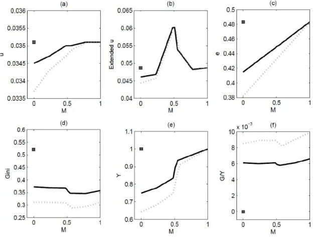
Figure 3 displays the effects of cash transfers on the economy (i.e, unemployment rate, extended unemployment rate, employment rate, Gini index, output, and government spending) for different levels of benefits and the coverage of the program. The square in each graph corresponds to the baseline case without any cash transfer. Observe that when the coverage of the program is small, cash transfers decrease both the unemployment and the employment rates.14Only when the eligibility of the program increases that the employment rate starts to increase. Some workers would receive benefits if they are working or not.15 Inequality decreases sharply. The Gini index decreases by roughly 30 percent with the introduction of cash transfers. However, inequality has a U-shape, since it starts to increase as more
13Total spending on cash transfers is:(1−e)b+bG(M)e.
14This is consistent with empirical findings. See, for instance, Hoynes (1996) who estimate how changes in benefit levels of the
program Aid to Families with Dependent Children affect labor supply in the United States.
15The model therefore could explain variation in the employment rate across countries by differences in the level of benefits
people become entitled to participate in this welfare program. Notice that output first decreases due to a decrease in the participation rate. However, as the employment rate increases with the coverage of the program, output starts to increase.16 Government spending as a share of income is roughly constant.
Figure 3: The effects of cash transfers on the economy. Black square: Baseline economy. Black solid line: b= 0.1yand different levels ofM. Gray dotted line:b= 0.15yand different levels ofM
Notice that as the level of benefits increase further the quantitative effects on the economy become stronger as well as on government finance.17When the eligibility of the program is low, the Gini index decreases by 15 percent when the level of benefits increases by 50 percent. Output, however, decreases by about 16 percent and government spending as a share of income in the welfare program increases by 35 percent. If the government target is to decrease inequality, the more efficient policy is to increase the level of benefits instead of increasing the eligibility of the program. However, such policy comes with a negative impact on efficiency (unless the majority of workers receive transfers) and on government finances.
supply and on home production. They use a consumer problem with a standard leisure-labor choice in which agents choose the allocation of their time endowment in leisure, market hours, and home production.
16As in Acemoglu et al. (2001), we are assuming that the taxes are financed by non-distortionary taxation. Results for aggregate
output might be different once we introduce distortionary taxes.
5. CONCLUDING REMARKS
This papers shows the effects of cash transfers on the labor market in a matching model with endogenous job destruction and labor market participation. In our model, the government provides cash transfers,b >0, to all workers with income less thanw, independently whether they are working, unemployed, or out of the labor force, i.e., working in home production. We also discuss the role of alternative policies, such as transfers conditional to labor market participation.
We show that the size of cash transfers has a negative effect on the employment rate, but an ambiguous effect on the unemployment rate. Participation rate is also affected negatively. In addition, the eligibility of the program has a positive effect on the employment rate, and an ambiguous effect on the unemployment rate. The numerical simulations show that the quantitative effects might be sizeable, specially on income inequality which decreases sharply with cash transfers. In order to avoid the negative effects on participation rate (and productivity) the government could also introduce a labor market participation program providing benefits for agents that are either working or searching for a job.18
There are some important extensions of this paper. First, it will be interesting, for instance, to inves-tigate the effects of cash transfers on the labor market using an alternative model with risk aversion in which agents accumulate assets, as the equilibrium search model of Alvarez and Veracierto (1999). Risk aversion would increase the welfare effects of cash transfers to the poor when agents cannot insure against idiosyncratic shocks. It will be also interesting to check whether or not the predictions of the model are consistent to the empirical evidence.
BIBLIOGRAPHY
Acemoglu, D., Johnson, S., & Robinson, J. A. (2001). The colonial origins of comparative development: An empirical investigation. American Economic Review, 91:1369–1401.
Alvarez, F. & Veracierto, M. (1999). Labor market policies in an equilibrium search model. 1999 NBER Macroeconomics Annual, 14:265–304.
Antunes, A. & Cavalcanti, T. (2007). Start up costs, limited enforcement, and the hidden economy.
European Economic Review, 51(1):203–224.
Bertola, G. & Rogerson, R. (1997). Institutions and labor reallocation. European Economic Review, 41(6):1147–1171.
Blanchard, O. & Diamond, P. (1989). The beveridge curve.Brookings Papers on Economic Activity, 1:1–76. Blanchard, O. & Portugal, P. (2001). What hides behind an unemployment rate: Comparing Portuguese
and US labor markets.American Economic Review, 91(1):187–207.
Cavalcanti, T. (2004). Layoff costs, tenure, and the labor market. Economics Letters, 84(3):383–390. Cavalcanti, T. & Corrêa, M. (2009). Cash transfers to the poor and the labor market. Mimeo, University of
Cambridge.
Currie, J. & Gahvari, F. (2008). Transfer in cash and in-kind: Theory meets the data. Journal of Economic Literature, 46(2):333–383.
18If we interpret the home production sector as the informal sector, this labor market program might be an effective mechanism
Diamond, P. (1982). Wage determination and efficiency in search equilibrium.Review of Economic Studies, 49(2):217–27.
Friedman, M. (1962). Capitalism and Freedom. The University of Chicago Press.
Garibaldi, P. & Wasmer, E. (2005). Equilibrium search unemployment, endogenous participation and labor market flows.Journal of the European Economic Association, 3(4):851–882.
Hoynes, H. W. (1996). Welfare transfers in two-parent families: Labor supply and welfare participation under AFDC-UP. Econometrica, 64(2):295–332.
Jones, S. R. G. & Riddell, W. C. (1999). The measurement of unemployment: an empirical approach.
Econometrica, 67(1):147–161.
Lindert, P. H. (2004). Growing Public: Social Spending and Economic Growth Since the Eighteenth Century, volume 1. Cambridge University Press.
Ljungqvist, L. (2002). How do layoff costs affect unemployment? Economic Journal, 112:829–853. Ljungqvist, L. & Sargent, T. (1998). The European unemployment dilemma. Journal of Political Economy,
106(3):514–550.
Mortensen, D. (1982). Property rights and efficiency in mating, racing and related games. American Economic Review, 72(5):968–979.
Mortensen, D. & Pissarides, C. (1994). Job creation and job destruction in the theory of unemployment.
Review of Economic Studies, 61:397–415.
Mortensen, D. & Pissarides, C. (1999). New developments in models of search in the labor market. In Ashenfelter, O. & Card, D., editors,Handbook of Labor Economics, volume 3, pages 2567–2627. Elsevier. Ngai, L. R. & Pissarides, C. (2008). Employment outcomes in the welfare state. Revue Economique,
59:413–436.
Pavoni, N. & Violante, G. L. (2007). Optimal welfare-to-work programs. Review of Economic Studies, 74(1):283–318.
Pissarides, C. (1990). Equilibrium Unemployment Theory. Oxford: Basil Blackwell.
Rogerson, R. (2007). Taxation and market work: is Scandinavia an outlier? Economic Theory, 32(1):59–85. Rogerson, R., Shimer, R., & Wright, R. (2005). Search-theoretic models of the labor market: A survey.
Journal of Economic Literature, 43(4):959–988.
Soares, F. V., Soares, S., Medeiros, M., & Osório, R. G. (2006). Cash transfer programmes in brazil: Impacts on inequality and poverty.United Nations Development Programme, Working Paper 21.
A. PROOF OF PROPOSITION 2.1
Using the implicit function theorem and Equation (11), we can show that:
∂EN B
∂b =
1
y
1 +r+ψψG(EN B)>0
Therefore,EN B > EB, sinceEN B =EB whenb = 0. Moreover,RN B−RB =EN B−EB,
B. PROOF OF PROPOSITION 3.1
Observe that, in the steady stateθ,EB, andRB do not depend onbandM. In addition,M does
not also affectEN BandRN B, however, from equations (11) and (10), we can show thatbaffectsEN B
andRN Bpositively, i.e., ∂EN B
∂b >0 ∂RN B
∂b >0.
From (20) and (21) we have that:
f1(e,u,b,M) = e− θq(θ)u
ψ{G(EB)G(M) +G(EN B)[1−G(M)]} = 0 (B-1)
f2(e,u,b,M) = u−(1−e)ψ{[1−G(R
B)]G(M) + [1−G(RN B)][1−G(M)]}
θq(θ) +ψ = 0 (B-2)
Observe that:
fe1= 1, fu1=− θq(θ)
ψ{G(EB)G(M) +G(EN B)[1−G(M)]} <0
fu2= 1, fe2=ψ{[1−G(R
B)]G(M) + [1−G(RN B)][1−G(M)]}
θq(θ) +ψ >0
Moreover,
fb1 = uθq(θ)G
′(EN B)[1−G(M)]∂EN B
∂b
ψ{G(EB)G(M) +G(EN B)[1−G(M)]}2 >0 fb2 = (1−e)ψG
′(RN B)[1−G(M)]∂RN B
∂b
θq(θ) +ψ >0 and
fM1 = − θq(θ)uG′(M)[G(E
N B)−G(EB)]
ψ{G(EB)G(M) +G(EN B)[1−G(M)]}2 <0 fM2 = −(1−e)ψG
′(M)[G(RN B)−G(RB)]}
θq(θ) +ψ <0
Since the determinant of the matrix with the derivative of functionsf1andf2with respect to the endogenous variableseanduis non-singular, we can use the implicit function theorem to show that:
∂e
∂b <0, and ∂u
∂b R0 ∂e