OCCUPATIONAL SEGREGATION AND THE GENDER
WAGE GAP IN BRAZIL: AN EMPIRICAL ANALYSIS
*Regina Madalozzo†
Abstract
Several countries experienced an increase in female labor participa-tion during the twentieth century. Even so, few can be proud of the con-ditions female workers faced. This paper analyzes the occupational dis-tribution by gender from 1978 to in 2007 in Brazil. It shows that women have penetrated traditionally male occupations to a certain extent, but that traditionally female occupations have maintained their gender com-position over the past 30 years. We also provide a regression analysis with an Oaxaca decomposition that shows that the gender wage gap is lower than in 1978, but that it has remained constant over the last decade.
Keywords:wage differentials, discrimination, and female labor market. Palavras-chave:diferenciais de salário, discriminação, mercado de traba-lho feminino
JEL classification:J24, J31, J71.
1
Introduction
Virtually all countries experienced an increase in female labor participation during the twentieth century. Even so, few can be proud of the conditions that female workers face in dealing with family responsibilities and the labor mar-ket. The division of labor within families continues to fall along traditional gender lines, even when women engage in labor market activities. Women who are engaged in the labor market are still expected to be available to
com-ply with theirfamily responsibilitiesof housework, childcare and other
activi-ties (Hersch & Stratton 1994,Alvarez et al. 2006,Lundberg 2008,Madalozzo
et al. 2008,Gupta & Ash 2008). Further, women continue to receive lower
wages than men, even when controlling for personal characteristics and job
attributes (Blau & Kahn 1997,Bertrand & Hallock 2001,Albrecht et al. 2003,
Bayard et al. 2003,Bucheli & Sanroman 2005,Galarza et al. 2006,Madalozzo
& Martins 2007,Olivetti & Petrongolo 2008). There is no consensus among
specialists as to whether a gendered division of labor at home causes the wage gap or vice versa. However, the majority of studies agree that some intrinsic
*This paper has benefited from the suggestions made by an anonymous referee and the excellent research assistance of Carolina Flores Gomes. The research was conducted with financial support from CNPq (Productivity Research Fellowship #307513/2007-6)
†Insper Instituto de Ensino e Pesquisa, email:[email protected]
features of gender have a significant influence on these outcomes of a lower wage and second shift.
One possibility is that the career interruptions that women experience
dur-ing their reproductive life1 make them less productive on the labor market
and, therefore, available to work for lower wage rates (Deloach & Hoffman
2002, Hersch & Stratton 2002, Moe 2003, Blau et al. 2006, Bryan & Sanz
2007). Another possibility is that women’s wages are lower because they ac-count for benefits that are available only to women, for example, maternity
leave (Waldfogel 1998,Edwards 2006,Bergmann 2008). As a final point,
an-other possibility is that women choose to work in occupations and activities
with lower remuneration than those chosen by men (Easterlin 1995,
Macpher-son & Hirsch 1995,Miller 2009). Any of these possibilities may impact – or
be impacted by – the gender division of labor by making it less costly to the household for women to spend more hours at home instead of men; if both spouses are equally productive to the market, but the husband receives higher remuneration for his work than his wife, he has a comparative advantage in
dedicating more time and effort to the market (Ferber 2003).
Our focus in this study is to analyze female labor participation in Brazil since the 1970s. Brazil is a highly unequal country in several aspects. It has one of the worst Gini indexes in the world, 0.567, and had the 10th worst
in-come distribution in the world in 2007. Concerning gender differences, Brazil
ranked 74th out of 127 countries in the 2007 World Economic Forum’s Gender
Gap index, with a score of 0.664.2 Using data from 1978 to 2007 will allow us
to understand two different problems related to women’s labor participation:
occupational segregation and the gender wage gap over time.
Female labor participation in Brazil increased substantially during the
sec-ond half of the twentieth century, as depicted in Figure1. In 1950, roughly
14 percent of females participated in the labor market. By 1980, this num-ber had nearly doubled to 27 percent. The 1980s was the decade that wit-nessed the biggest inclusion of women in the labor market and by 1992, 47 percent of women were engaged in some economic activity or were seeking work. Since them, female inclusion in the labor market has slowly continued to grow. In 2007, 52.4 percent of women were economically active. Nev-ertheless, women’s working conditions in the labor market and within their households has remained inequitable.
Other studies have analyzed labor market conditions for women in Brazil.
Bruschini (1989, 1998) reported the trends for the female labor market
re-garding insertion and intermittency. The present research continues these analyses into the new century. In addition, we use econometric resources to evaluate female entries into industry and occupations and to compare
fe-male and fe-male wages, controlling for individual characteristics. Giuberti &
Menezes-Filho(2005),Jacinto(2005) andBatista & Cacciamali(2009) all used
the Oaxaca-Blinder methodology to compare earning differentials between
men and women, though each of these studies had a different focus.3
Com-1Labor intermittency caused by marriage, childbirth or other family needs involving the woman.
2Where one represents complete equal treatment between genders and zero, total inequal-ity. The gender gap index considers four dimensions: economic participation and opportunity, educational attainment, health and survival, and political empowerment.
0 10 20 30 40 50 60 70 80
1950 1960 1970 1980 1990 2000
female male
Source: IBGE, Estatísticas do Século XX
Figure 1: Labor Market Participation. Male and Female, 1950– 2007.
plementing their work, we expanded the period analyzed and emphasized the role of occupation choice in wage profiles. Our analyses target the average dif-ferences in labor market earnings for men and women for the period between
1978 and 2007. Finally,Scorzafave & Pazello (2007) also studied the gender
wage gap in Brazil, however their goal was to apply normalized equations to solve the indetermination problem of the Oaxaca-Blinder decomposition ap-proach. We use their methodology in our research to better understand the impact of the occupation transition process on narrowing the gender wage
gap during this period.4
This paper is organized as follows: in the next section we describe
Brazil-ian labor characteristics, focusing on activities and gender differentials.
Sec-tion 3 explains the empirical model used to analyze the gender gap in
remu-neration and the impact of occupational differentials. The results are
pre-sented in Section 4. Section 5 offers conclusions.
2
The Brazilian labor market: are there gender di
ff
erences?
In this section, we describe Brazilian labor markets and highlight the diff
er-ences and similarities between genders with regard to them. Before entering into such a discussion, however, it is necessary to explain some peculiarities of the Brazilian labor market. First, it is highly regulated. Since the 1930s, with the implementation of the first laws concerning employment in Brazil, there have been an increased number of restrictions and fees employers must pay to be able to hire individuals. The constitution of 1988 aggravated this problem. Second, women have gained specific rights to maternity leave. Be-fore 1988, all female workers had the right to a fully paid maternity leave of 90 days. The new constitution increased this right to 120 days. In 2007,
new federal legislation was passed in response to the World Health Organiza-tion’s recommendation that babies should be breastfed for 6 months. Under this law, female workers may opt to take 6 months of maternity leave, also
fully paid by the employer.5 These stringent regulations on the labor market
are the concern of many researchers, who question their ability to guarantee workers’ rights by suggesting that such regulations may force workers into informal jobs, where they will have no rights at all.
Our analysis used microdata from PNAD (Pesquisa Nacional de Amostra
por Domicílios, which translates to National Survey of Sampled Households).
PNAD is an annual survey conducted by the Brazilian Bureau of Statistics, IBGE. It takes a representative sample of Brazilian households and studies, among other aspects of the population, labor, education and health. It con-tains data at an individual level for the sampled dwellings. Since 2004, PNAD
has investigated data for all national territory.6 With the purpose of
analyz-ing the past and current employment trends, we used data from four different
decades: 1978, 1988, 1998, and 2007, the most recent data released by IBGE. Questionnaires were modified during this period; however, we made some concatenations in order to make them comparable.
Table1presents the female distribution among different occupation
cat-egories.7 For each year, we divided the occupations into traditionally male
or traditionally female.8 It can be observed that the majority of
occupa-tions remain majority male over time (for example, carpenters, mechanics, drivers, etc.), while others maintain their tendency to be female-dominated occupations (including nurses, librarians, and schoolteachers). Nevertheless, some changes are visible. While in 1978 only 4.94 percent of engineers were women, in 2007 more than 10 percent of engineers were female. This is still a small number of individuals; however, it establishes a change in pattern. Other examples of traditionally male occupations that are being occupied by increasing numbers women are insurance agents, police and detectives, and managers and administrators.
On the other side, traditionally female occupations rarely present such a change. There are a few possible explanations for this phenomenon. The first is that men resist engaging in activities that are regarded as “female.” This would reflect gender preferences for certain activities and against others. His-torically, women engaged in market activities closely related to their domestic work (Folbre 1994). Considering that men have historically been distant from
such work, it is plausible to infer that males would prefer a different type
of activity and, therefore, favor traditionally male occupations.It may also be
the case that this difference is related to worker discrimination (Kaufman &
Hotchkiss 2003). This would be the case if men charged a premium to work
5Up to a ceiling of 12 thousand Reais, maternity leave is paid by the employer who is reim-bursed by the government in taxes. This is a very high ceiling. Less than 3 percent of female workers earn more than this value monthly.
6Until then, 1.9 percent of the Brazilian population was not included in the sample because they lived in areas not researched. However, the analysis contains weights that allow for compar-ison with earlier years.
7This table was inspired by Table 8.3, inKaufman & Hotchkiss(2003, p.425).
Table 1: Percentage of females in traditionally male and traditionally female occupations.
Traditionally Male Occupations
Occupation 1978 1988 1998 2007
Engineers 4.94
[4,778] 2[455].47 [158.,35682] [2910,.382]08
Lawyers 18.18
[15,386] 25[3,708].86 [10438.,003]40 [20743.,86225]
Physicians 18.29
[14,144] 22[4,285].07 [10648.,848]15 [9642,.607]87
Economists 18.76
[3,864] 16[665].84 [1332,451].44 [22876.,13013]
Clergy 20.54
[5,249] 14[1,060].25 [2427,984].79 [3324,.676]96
Insurance agents 10.46
[2,424] 0[0].00 [1428,625].69 [3232,.178]69
Managers and administrators 16.77
[92,505] [2617,.282]10 [29528.,689]59 [136,609.48,614]
Carpenters 1.05
[2,011] 0[207].28 [132.,20349] [82,.108]04
Auto mechanics 0.29
[1,110] [11,.132]19 [30,.351]47 [91,.286]36
Telephone line installers 0.76
[195] 0[0].00 [16,.620]28 [33,.393]05
Drivers 0.17
[2,070] 0[895].40 [251.,20395] [391.,59580]
Police and Detectives 2.28
[1,746] 11[1,348].86 [1711,188].71 [2712,.822]23
Traditionally Female Occupations
Occupation 1978 1988 1998 2007
Registered nurses 86.94
[247,258] [4089,.139]92 [5986,379].83 [8786,.428]48
Librarians 89.56
[14,847] 82[3,595].10 [1492,769].55 79[4,259].41
Schoolteachers 90.58
[796,709] [8888,.539]87 [191,261.41,264] [181,942.54,572]
Bank tellers 54.70
[119,922] [3872,.834]43 [11551.,502]94 [4955,.831]51
Secretaries 52.23
[944,816] [3698,.688]26 [19461.,194]48 [162,362.39,068]
Typists 37.04
[56,654] 26[2,699].25 [37291.,472]82 13[6,007].40
Sewing machine operators 95.17
[844,866] [14497.,00360] [193,200.54,793] [191,213.99,158]
Dental assistants 22.53
[10,467] 22[2,303].87 [5653,295].49 [9055,.547]27
Child care workers − 100.00
[6,739] [40797.,142]86 [30597.,76128] Source: PNADs and author’s tabulation.
with women in a “female job.” In that case, the premium could be so high that firm owners prefer to hire only women because they are less costly. An-other alternative is that society resists having men in these occupations. For example, male nurses may be less socially desirable than female nurses. A man who chooses to become a nurse may be viewed as a “failed doctor” more
easily than a woman.9 This explanation is commonly known as “consumer
prejudice” (Patterson & Engelberg 1978).
These differences in occupations and industry choices may be
determi-nants of the remuneration discrepancy between genders. In order to better
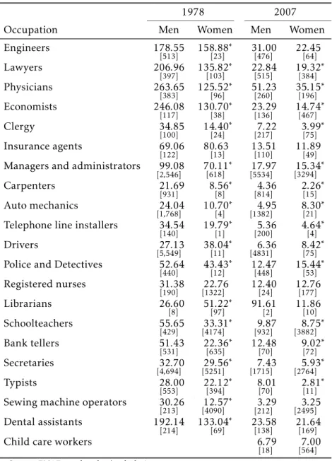
control this effect, Table2provides the individuals’ hourly pay by occupation
and gender10for 1978 and 2007. Table3does the same for economic sector
and gender.
Using the same categories analyzed in Table1, it can be seen that, in most
cases, men have higher salaries than women. In 1978, for only two occupa-tions, drivers and librarians, did females have a higher average salary than males. For another 16 occupations, men received higher remuneration than
women. In 2007, the situation is slightly different: in 12 occupations, men
earn greater wages than women and, for three others, women earn higher wages than men (auto mechanics, drivers, and police and detectives). With no controls for education and industry, which we examine in the next section, it appears that there has been little change in the gender wage gap over a long period of time.
Concerning industry sectors, Table3 shows that men typically received
higher wages than women in the past. However, in one activity, women’s salaries are higher: construction. This is also one of the activities with lower female engagement. One possible explanation for this premium on female wages is individual selection. In order to participate in this industry, women
have to be so different from the average that they receive higher wages than
men. Analyzing the education distribution among industries, it can be seen that in the construction industry women are more educated than men. In 1978, almost 60 percent of females in the construction industry had 9 or more years of education (completed the primary level of education), while less than 8 percent of males in this industry had this level of education. In 2007, 68 percent of women in this industry had more than 9 years of education, while 21 percent of men were in the same condition.
This question raises the importance of analyzing the degree of education.
Comparing 1978 and 2007 data, we can see some different trends by gender
in Table4. In 1978, men with a low level of education were concentrated in
the agribusiness sector. Women with no education were also in agribusiness, but those who had a small amount of education (1 to 4 years) were in services. Men who had 5 to 11 years of education were in the transformation indus-try, while women at this level were generally in the services and the social sector. Individuals of both genders with more than 11 years of education are
more concentrated in the social sector. The picture in 2007 is a little diff
er-ent. Men with low education levels continue to work in agribusiness (until 4 years of education), and women in services. However, after finishing the basic
9Anecdotal evidence of this can be seen in the Hollywood hit movie “Meet the Parents,” where the parents of the fiancée avoid saying that their future son-in-law is a nurse.
Table 2: Hourly wage by gender and occupation: 1978 and 2007.
1978 2007
Occupation Men Women Men Women
Engineers 178.55
[513] 158[23].88
∗ 31.00
[476] 22[64].45
Lawyers 206.96
[397] 135[103].82
∗ 22.84
[515] 19[384].32
∗
Physicians 263.65
[383] 125[96].52
∗ 51.23
[260] 35[196].15
∗
Economists 246.08
[117] 130[38].70
∗ 23.29
[136] 14[467].74
∗
Clergy 34.85
[100] 14[24].40
∗ 7.22
[217] 3[75].99
∗
Insurance agents 69.06
[122] 80[13].63 13[110].51 11[49].89
Managers and administrators 99.08
[2,546] 70[618].11
∗ 17.97
[5534] [3294]15.34
∗
Carpenters 21.69
[931] 8.[8]56
∗ 4.36
[814] 2[15].26
∗
Auto mechanics 24.04
[1,768] 10.[4]70
∗ 4.95
[1382] 8[21].30
∗
Telephone line installers 34.54
[140] 19.[1]79
∗ 5.36
[200] 4.[4]64
∗
Drivers 27.13
[5,549] 38[11].04
∗ 6.36
[4831] 8[75].42
∗
Police and Detectives 52.64
[440] 43[12].43
∗ 12.47
[448] 15[53].44
∗
Registered nurses 31.38
[190] [1322]22.76 12[24].40 12[177].76
Librarians 26.60
[8] 51[97].22
∗ 91.61
[2] 11[10].86
Schoolteachers 55.65
[429] [4174]33.31
∗ 9.87
[932] [3882]8.75
∗
Bank tellers 51.43
[531] 22[635].36
∗ 12.48
[70] 9[72].02
∗
Secretaries 32.70
[4,694] [5251]29.56
∗ 7.43
[1715] [2764]5.93
∗
Typists 28.00
[553] 22[394].12
∗ 8.01
[70] 2[11].81
∗
Sewing machine operators 30.26
[213] [4090]12.57
∗ 3.29
[212] [2495]3.25
Dental assistants 192.14
[214] 133[69].04
∗ 23.58
[138] 21[169].64
Child care workers 6.79
[18] [564]7.00 Source: PNADs and author’s tabulation.
All estimations are weighted by the individual weight available in the database.
Table 3: Hourly wage by gender and industries: 1978 and 2007.
1978 2007
Activity Men Women Men Women
Agricultural 14.86 6.49∗ 3.10 0.91∗
Transformation Industry 38.11 17.42∗ 7.12 4.33∗
Construction 23.21 38.82∗ 4.72 19.72∗
General Industry 31.46 33.10 10.45 11.02
Commerce 38.26 21.81∗ 6.48 4.83∗
Services 40.00 12.30∗ 7.65 3.56∗
Transportation 32.67 26.39∗ 7.28 7.45
Social Services 74.35 32.77∗ 13.45 8.26∗
Public Administration 50.08 45.15∗ 12.02 10.99∗
Other Activities 78.14 38.85∗ 9.12 7.04∗
Source: PNADs and author’s tabulation.
All estimations are weighted by the individual weight available in the database.
∗female and male values are different at the 95 percent confidence interval.
level of education, i.e., 4 years, men are employed in commerce. Women, for their part, continue to be concentrated in services until completing the fun-damental level of education, i.e., 8 years, and after that, they compose a larger fraction of commerce.
3
Econometric model to calculate discrimination between
genders
The previous analysis illustrates that male and female workers have different
allocations within and returns to the labor market in Brazil. We now present an econometric analysis in order to control for distinct influences on individ-ual remuneration. Using this procedure, we will also be able to measure the impact of occupational choices and individual characteristics on the hourly wage.
The basic model followsMincer(1995). The mincerian equation relates
the hourly wage with individual demographics and job definitions, as shown by equation (1).
lnwi=α+
k X
j=1 βjXi+
m X
s=1
γsZi+εi, (1)
wherewi is the hourly wage for individualiandXi are the demographics for
individuali.Zi represents dummy variables for activities and occupations for
each individual11.
By demographics, we mean individual age and its squared value (to
ac-count for the concavity on remuneration), residence region12 and education
dummies.13 Zi is composed of both occupation and industry dummies. For
11Excluded category is Agricultural Business.
12Excluded category is Southeast, the richest Brazilian region.
1978
years of education
0 1 to 4 5 to 8 9 to 11 12 + Male Workers
Agribusiness 62.82 30.92 9.28 3.39 1.39 Transformation 8.67 19.73 24.87 24.65 19.92 Construction 11.40 14.71 9.71 4.78 5.54 Other industrial activities 1.86 2.38 2.13 3.22 3.13 Commerce 5.45 9.75 15.55 17.10 7.66 Services 4.68 9.82 14.59 13.57 15.05 Transportation and Communication 2.68 6.87 9.47 6.17 3.34 Social 0.74 1.77 3.50 5.63 21.03 Public Administration 1.10 2.99 7.87 10.39 13.23 Other activities 0.59 1.07 3.03 11.11 9.71
Female Workers
Agribusiness 49.00 23.37 5.55 0.37 0.06 Transformation 6.71 14.00 17.68 11.16 6.89 Construction 0.10 0.24 0.47 1.29 1.55 Other industrial activities 0.32 0.28 0.31 1.05 1.56 Commerce 3.72 7.82 17.25 12.85 4.08 Services 35.87 42.26 31.07 12.27 7.70 Transportation and Communication 0.20 0.72 1.90 2.78 2.03 Social 2.65 8.95 20.00 43.35 57.74 Public Administration 0.39 1.06 3.33 7.35 10.46 Other activities 1.04 1.29 2.43 7.55 7.94
2007
years of education
0 1 to 4 5 to 8 9 to 11 12 +
Male Workers
Agribusiness 53.37 35.28 15.30 5.78 1.82 Transformation 7.95 12.11 18.36 21.93 13.70 Construction 14.54 18.55 16.50 7.07 3.43 Other industrial activities 0.84 0.93 1.13 1.83 1.66 Commerce 9.84 13.20 21.04 24.69 16.05 Services 2.86 3.27 3.72 3.95 4.86 Transportation and Communication 3.75 6.87 9.91 9.07 5.20 Social 0.67 1.01 1.40 3.53 16.42 Public Administration 2.03 2.67 3.12 7.89 13.38 Other activities 4.15 6.09 9.51 14.25 23.47
Female Workers
Agribusiness 44.39 31.19 11.32 2.93 0.59 Transformation 8.12 11.74 16.08 14.21 6.87 Construction 0.29 0.36 0.35 0.55 0.95 Other industrial activities 0.11 0.07 0.11 0.26 0.68 Commerce 8.32 9.43 15.36 25.48 11.86 Services 27.98 33.26 36.66 18.25 4.78 Transportation and Communication 0.31 0.42 0.85 2.43 2.55 Social 3.51 5.16 6.59 17.70 44.52 Public Administration 1.25 1.46 2.10 5.21 10.67 Other activities 5.71 6.90 10.57 12.98 16.53
Source: PNADs and author’s tabulation.
all years, we used the classification of these variables on two and three-digit dummies. Here, it is necessary to point out the endogeneity of these latter variables, especially occupation. It is well known that occupational choices are made according to individual preferences, and that such choices imply
different levels of remuneration, linking the dependent variable with this
in-dividual choice. An instrumental variable could be used to correct for this problem. Unfortunately, the database used in this study does not allow for the construction of such a variable. Therefore, we continue to control for
oc-cupation and industry choice while ignoring this possible effect, but using the
same methodology used in the literature.
We were also able to test for the influence of occupational distinction of
authority on wages.Budig & England(2001) created a dummy variable for
au-thority in their study on the wage penalty of motherhood. This variable was constructed by coding all occupations that have the words “management,” “supervisor” or “foreman” in their description as one. As a dependent vari-able, they used the natural log of hourly wage in the respondent’s current job. They find that mothers are less likely to be in jobs involving authority;
however, this does not seem to affect the estimated motherhood penalty. In
our work, “authority” was included as a variable of job characteristics. This variable is a dummy, coded one for occupational categories with titles contain-ing the words “supervisor,” “manager” or “director.” We used this additional variable only for the 2007 data, which is more complete. Also, for 2007, we
included race dummies14 and tenure on the job15 in order to have a more
complete set of controls.16
Since the main purpose of this study is to analyze female labor characteris-tics, we estimated equation (1) separately for men and women using ordinary least squares. We did not use a Heckman correction for the female equation
because we are concerned only with working individuals.17 These regressions
result in two different outcomes, posed as equations (2) and (3).
lnwFi = ˆαF+
k X
j=1
ˆ
βFjXiF+
m X
s=1
ˆ
γsFZiF+εi (2)
lnwMi = ˆαM+
k X
j=1
ˆ
βMj XiM+
m X
s=1
ˆ
γsMZiM+εi, (3)
where equation (2) uses only female data to estimate the coefficients, and
equation (3) uses the male data to this end. These features allow us use the
Oaxaca(1973) method to estimate the male–female differences not explained
by individual characteristics.
14Excluded category is White; other categories are Black, Mulato, Asian and Native.
15Excluded category is “less than 6 months”; other categories are “6 months to 1 year,” “1 to 2 years,” “2 to 5 years” and “more then 5 years.”
16Since 1976, IBGE changed the PNAD questionnaires many times. We do not have all of the basic variables for all years. Therefore, we estimated a more complete equation only for 2007, but kept the “basic” regression for all years for comparison.
and women) and the unexplained di erential.
Using the estimated coefficients for female and male individuals, we
cal-culate the hourly wage one individual would receive if he or she were male and, the alternative possibility, if he or she were female. We use these
compu-tations to determine the wage differential that is not explained by observable
characteristics, as shown in equation (4):
ˆ
Di= X
j
ˆ
βjMXi−
X
j
ˆ
βjFXi. (4)
We compare the estimated value of equation (4) for each individual and use the population average for this variable as the estimation of the non-explained portion of the gender wage gap across the years. The greater the
value of the difference in the sample, the greater the gender discrimination in
the sample.18 In the next section, we present the results.
4
And the di
ff
erence between genders is. . .
We estimate equations (2) and (3) separately for the different samples (1978,
1988, 1998 and 2007). As mentioned earlier, for 2007, because of the avail-ability of additional variables, we included extra controls for race, tenure and authority. Our baseline regression includes demographics, industry sector and two-digit occupational controls. The final model also includes
occupa-tional codes with three digits.19 All of our estimations were calculated using
the individual weight available in the PNAD, as well as robust standard errors to correct for heteroscedasticity.
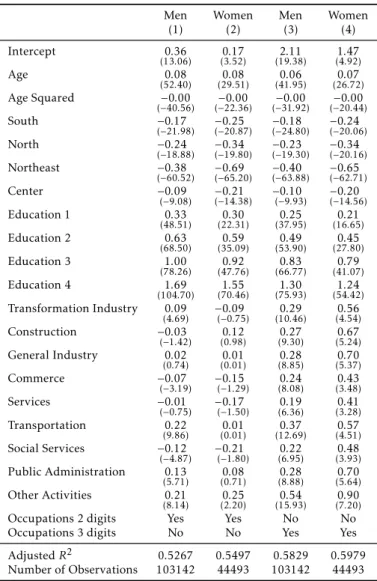
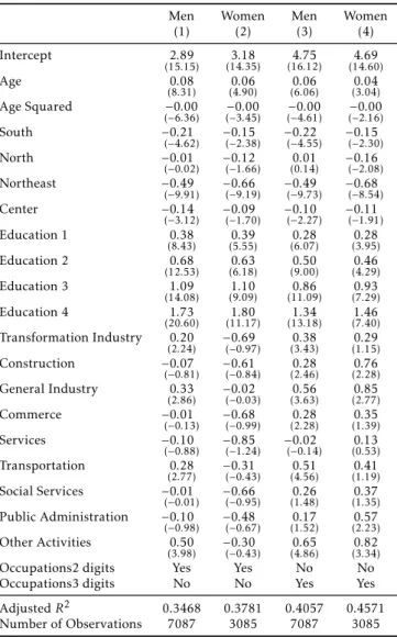
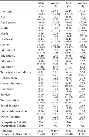
Tables5through8show the estimated results, disaggregated by gender.
Columns (1) and (3) refer to the male results, and columns (2) and (4) refer to
female results. For all years, we find a positive effect of age, with concavity
expressed by the variable age squared. These effects are expected, because
they reflect the worker’s experience with the labor market. The concavity is verified because the incremental value of experience along the years has decreasing returns to productivity and, consequently, to individual remuner-ation. Some studies use the age variable as a proxy for experience. However, this is not a good approach to infer women’s labor experience, because they experience time out of the labor market to have and raise children. Therefore, the variable “age” measures the impact of age itself, more so than labor ex-perience. In order to have some control for labor experience, the regression
18The D statistic can either be an overestimation or underestimation of discrimination. Not all of the differences verified on variable D can be considered discrimination per se. As the available microdata are not complete for the individual characteristics, we only can affirm that we control for the “observable” characteristics of each individual, and the D statistic represents the effect of “non-observable” characteristics available to neither the researcher nor the labor contractors. Therefore, any remaining differences would be the result of some sort of gender discrimination. On the other hand, D may underestimate the discrimination because we control for characteristics like occupation, and, if there is non-market discrimination that induces women to opt for easier and worse remunerated occupations, we would not see it on the final estimation. SeeOaxaca
(1973).
Table 5: Estimation Results, 1978.
Men Women Men Women
(1) (2) (3) (4)
Intercept 0.36
(13.06) (30..1752) (192.11.38) (41..4792)
Age 0.08
(52.40) (290.08.51) (410.06.95) (260.07.72) Age Squared −0.00
(−40.56) (−22−0.00.36) (−31−0.00.92) (−20−0.00.44)
South −0.17
(−21.98) −(−200.25.87) (−24−0.18.80) (−20−0.24.06)
North −0.24
(−18.88)
−0.34
(−19.80)
−0.23
(−19.30)
−0.34
(−20.16) Northeast −0.38
(−60.52) −(−650.69.20) (−63−0.40.88) (−62−0.65.71)
Center −0.09
(−9.08)
−0.21
(−14.38) −(−90.10.93) (−14−0.20.56) Education 1 0.33
(48.51) (220.30.31) (370.25.95) (160.21.65) Education 2 0.63
(68.50) (350.59.09) (530.49.90) (270.45.80) Education 3 1.00
(78.26) (470.92.76) (660.83.77) (410.79.07) Education 4 1.69
(104.70) (701.55.46) (751.30.93) (541.24.42) Transformation Industry 0.09
(4.69) −(−00.09.75) (100.29.46) (40..5654) Construction −0.03
(−1.42) (00..1298) (90..2730) (50..6724) General Industry 0.02
(0.74) (00..0101) (80..2885) (50..7037) Commerce −0.07
(−3.19) −(−10.15.29) (80..2408) (30..4348) Services −0.01
(−0.75) −(−10.17.50) (60..1936) (30..4128) Transportation 0.22
(9.86) (00..0101) (120.37.69) (40..5751) Social Services −0.12
(−4.87) −(−10.21.80) (60..2295) (30..4893) Public Administration 0.13
(5.71) (00..0871) (80..2888) (50..7064) Other Activities 0.21
(8.14) (20..2520) (150.54.93) (70..9020) Occupations 2 digits Yes Yes No No Occupations 3 digits No No Yes Yes
AdjustedR2 0.5267 0.5497 0.5829 0.5979 Number of Observations 103142 44493 103142 44493
Between parentheses are thet-statistics for each coefficient. All regressions have robust standard errors estimations
All estimations are weighted by the individual weight available in the database.
for 2007 also includes the variable “tenure on the job,” which captures part of
this effect.
The second variable category is the regional dummies. Except for 2007, Southeast, the excluded category, has the greatest positive impact on wages for both men and women. In 2007, it is possible to verify that Center is the region with higher wages for both men and women in all regressions. This
may be an effect of migration to the Southeast, which began in the 1960s and
stabilized at the end of the 1990s as growth registered in the Central region,
which was poorly occupied until the end of the 1980s.20
Table 6: Estimation Results, 1988.
Men Women Men Women
(1) (2) (3) (4)
Intercept 2.89
(15.15) (143.18.35) (164.75.12) (144.69.60)
Age 0.08
(8.31) (40..0690) (60..0606) (30..0404) Age Squared −0.00
(−6.36) (−3−0..45)00 (−4−0..61)00 (−2−0..16)00
South −0.21
(−4.62)
−0.15
(−2.38)
−0.22
(−4.55)
−0.15
(−2.30)
North −0.01
(−0.02) −(−10.12.66) (00..0114) −(−20.16.08) Northeast −0.49
(−9.91) −(−90.66.19) −(−90.49.73) −(−80.68.54)
Center −0.14
(−3.12) −(−10.09.70) −(−20.10.27) −(−10.11.91) Education 1 0.38
(8.43) (50..3955) (60..2807) (30..2895) Education 2 0.68
(12.53) (60..6318) (90..5000) (40..4629) Education 3 1.09
(14.08) (91..1009) (110.86.09) (70..9329) Education 4 1.73
(20.60) (111.80.17) (131.34.18) (71..4640) Transformation Industry 0.20
(2.24) −(−00.69.97) (30..3843) (10..2915) Construction −0.07
(−0.81) −(−00.61.84) (20..2846) (20..7628) General Industry 0.33
(2.86) −(−00.02.03) (30..5663) (20..8577) Commerce −0.01
(−0.13) −(−00.68.99) (20..2828) (10..3539) Services −0.10
(−0.88) −(−10.85.24) −(−00.02.14) (00..1353) Transportation 0.28
(2.77) −(−00.31.43) (40..5156) (10..4119) Social Services −0.01
(−0.01) −(−00.66.95) (10..2648) (10..3735) Public Administration −0.10
(−0.98) −(−00.48.67) (10..1752) (20..5723) Other Activities 0.50
(3.98) −(−00.30.43) (40..6586) (30..8234)
Occupations2 digits Yes Yes No No
Occupations3 digits No No Yes Yes
AdjustedR2 0.3468 0.3781 0.4057 0.4571 Number of Observations 7087 3085 7087 3085
Between parentheses are thet-statistics for each coefficient. All regressions have robust standard errors estimations
Table 7: Estimation Results, 1998.
Men Women Men Women
(1) (2) (3) (4)
Intercept −1.78
(−52.83) −(−351.72.25) −(−60.45.43) −(−10.60.63)
Age 0.07
(40.32) (230.06.79) (340.06.23) (200.05.67) Age Squared −0.00
(−31.77) (−17−0.00.10) (−27−0.00.07) (−15−0.00.09)
South −0.08
(−10.11) −(−170.09.10) (−10−0.08.41) −(−100.10.08)
North −0.26
(−21;64) −(−80.26.72) (−22−0.26.11) −(−190.27.18) Northeast −0.43
(−57.64)
−0.50
(−17.79)
−0.42
(−58.18)
−0.48
(−53.59)
Center −0.09
(−8.65) −(−530.12.54) −(−80.09.87) −(−100.12.33) Education 1 0.25
(25.13) (120.20.85) (200.20.61) (100.16.78) Education 2 0.49
(45.02) (240.40.30) (350.38.44) (200.33.47) Education 3 0.80
(64.65) (370.69.85) (510.64.19) (310.57.81) Education 4 1.46
(86.54) (621.32.86) (631.12.92) (481.03.04) Transformation Industry 0.21
(7.94) (10..1121) (70..1666) (40..2042) Construction 0.11
(4.00) (20..2327) (40..0913) (50..3494) General Industry 0.28
(8.74) (20..2215) (100.31.60) (80..5326)
Commerce 0.12
(4.30) (10..0901) (40..1034) (40..1904)
Services 0.10
(3.74) −(−00.02.20) −(−10.03.22) (10..0998) Transportation 0.38
(13.67) (3;38)0.33 (110.25.07) (60..3527) Social Services 0.10
(3.50) −(−00.01.07) (30..1082) (40..1933) Public Administration 0.34
(12.31) (20..2453) (30..0707) (60..3048) Other Activities 0.25
(9.23) (20..2679) (70..1623) (70..3425) Occupations 2 digits Yes Yes No No Occupations 3 digits No No Yes Yes AdjustedR2 0.5177 0.4994 0.57 0.5627 Number of Observations 70440 43320 70440 43320
Between parentheses are thet-statistics for each coefficient. All regressions have robust standard errors estimations
O cc u p at io n al Se gr eg at io n 16 1
Age 0.06
(36.94) (240.05.69) (330.05.94) (230.05.81) (310.05.40) (190.04.97) (280.05.94) (190.04.23)
Age Squared −0.00
(−27.09)
−0.00 (−17.67)
−0.00 (−25.06)
−0.00 (−16.84)
−0.00 (−23.69)
−0.00 (−14.94)
−0.00 (−21.89)
−0.00 (−14.15)
Black - - - - −0.14
(−14.92)
−0.07 (−6.34)
−0.12 (−13.18)
−0.05 (−4.83)
Mulato - - - - −0.12
(−21.31)
−0.10 (−15.00)
−0.11 (−19.22)
−0.08 (−12.67)
Asian - - - - 0.06
(1.28) 0(2.11.76) 0(1.08.73) 0(2.09.43)
Native /Indigenous - - - - −0.13
(−3.01)
−0.03 (−0.50)
−0.11 (−2.69)
−0.03 (−0.58)
Manager Position - - - - 0.20
(15.45) (100.28.81) −(0−.154.01) 0(1.66.17)
South 0.01
(0.88) −(0−.101.21)
0.01
(1.07) −(0−.001.46)
−0.02 (−2.93)
−0.03 (−3.35)
−0.01 (−2.05)
−0.02 (−2.16)
North −0.12
(−15.33)
−0.17 (−17.20)
−0.10 (−12.50)
−0.15 (−15.87)
−0.09 (−10.60)
−0.14 (−13.74)
−0.07 (−8.36)
−0.12 (−12.76)
Northeast −0.43
(−62.23)
−0.42 (−53.02)
−0.40 (−59.45)
−0.39 (−51.48)
−0.40 (−57.30)
−0.40 (−49.77)
−0.38 (−54.85)
−0.38 (−48.52)
Center 0.04
(4.84) 0(0.01.86) 0(3.03.93) 0(1.02.67) 0(7.06.26) 0(2.02.28) 0(6.05.22) 0(2.03.94)
Education 1 0.19
(16.89) 0(9.17.05) (140.17.78) 0(8.15.35) (150.18.95) 0(8.16.68) (140.16.22) 0(8.15.10)
Education 2 0.40
(34.10) (180.35.62) (290.34.20) (160.30.56) (320.38.65) (170.34.95) (280.33.40) (160.29.14)
Education 3 0.63
(51.79) (290.56.22) (440.54.07) (250.47.43) (490.60.69) (270.53.91) (420.52.98) (240.45.62)
Education 4 1.14
(73.62) (491.04.06) (620.98.03) (410.86.58) (701.09.68) (460.99.89) (600.95.37) (400.83.30)
Tenure on the job 1 - - - - 0.06
(5.52) 0(4.06.72) 0(5.06.54) 0(5.06.09)
Tenure on the job 2 - - - - 0.06
(6.10) 0(8.10.74) 0(6.06.39) 0(9.10.01)
Tenure on the job 3 - - - - 0.10
(10.70) (140.16.60) (100.09.90) (150.16.00)
Tenure on the job 4 - - - - 0.20
R
eg
in
a
M
ad
al
oz
zo
E
co
n
om
ia
A
p
lic
ad
a,
v.1
4
,
n
.2
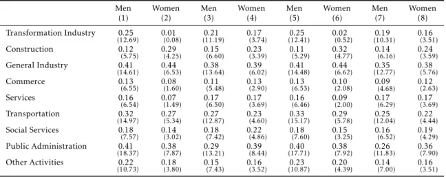
Table 8: Estimation Results, 2007. (continued)
Men Women Men Women Men Women Men Women
(1) (2) (3) (4) (5) (6) (7) (8)
Transformation Industry 0.25
(12.69) 0(0.01.08) (110.21.19) 0(3.17.74) (120.25.41) 0(0.02.52) (100.19.31) 0(3.16.51)
Construction 0.12
(5.75) 0(4.29.25) 0(6.15.60) 0(3.23.39) 0(5.11.29) 0(4.32.77) 0(6.14.16) 0(3.24.59)
General Industry 0.41
(14.61) 0(6.44.53) (130.38.64) 0(6.39.02) (140.41.48) 0(6.44.62) (120.35.77) 0(5.38.76)
Commerce 0.13
(6.55) 0(1.08.60) 0(5.11.48) 0(2.13.90) 0(6.13.53) 0(2.10.08) 0(4.09.68) 0(2.12.63)
Services 0.16
(6.54) 0(1.07.49) 0(6.17.50) 0(3.17.69) 0(6.16.46) 0(2.09.00) 0(6.17.29) 0(3.17.69)
Transportation 0.32
(14.97) 0(5.27.34) (120.27.87) 0(4.23.60) (150.33.17) 0(5.29.78) (120.25.04) 0(4.22.44)
Social Services 0.18
(7.57) 0(3.14.02) 0(7.18.42) 0(4.22.86) 0(7.18.60) 0(3.15.25) 0(6.16.52) 0(4.19.29)
Public Administration 0.41
(18.37) 0(7.38.87) (130.29.21) 0(8.39.44) (170.40.71) 0(7.38.92) (110.26.83) 0(7.36.90)
Other Activities 0.22
(10.73) 0(3.18.80) 0(7.15.43) 0(3.16.52) (100.23.87) 0(4.20.39) 0(7.14.00) 0(3.16.51) Between parentheses are thet-statistics for each coefficient. All regressions have robust standard errors estimations
tently greater for males than females throughout the categories and years. Finally, there is the occupation and industry impact on wages. We used
two different types of classification for occupational choice. The usual and
more appropriate one has a three-digit classification. Because it has too many groups, its analysis is excessively intricate. Therefore, for each year, we run a regression with occupational choice divided on two-digit and three-digit
classifications.22 Columns (1) and (2) in Tables5through7display the former
results and columns (3) and (4) of each table display the latter ones. Table8,
regarding 2007 data, has more columns, to include controls that were not
available on previous years. Therefore, in Table8, the controls for occupation
in columns (1), (2), (5) and (6) have a two digit classification and the other columns have a three digit classification. The more restricted classification of occupation interferes with the results of other variables. This is true for the
results by industry, which is our next focus.23
Industry indicators are fewer, and we can see a tendency in the estimated
coefficients. For males, the industrial sector pays more. For females,
pub-lic administration confers more wage benefits than other occupations. These
effects may be a combination of discrimination with a gender comparative
ad-vantage. Bergmann(1974) established a model to test the profitability
func-tion of occupafunc-tion discriminafunc-tion against its sociological purpose. She con-cluded that the latter may have a bigger influence on decision-makers. Using her model, we can conclude that activities with a greater social impact appear to suit women better, and that those where technical appeal is stronger suit men better. Therefore, recruiters prefer to place individuals in jobs associated with the characteristics of their gender (Hochschild 2003).
It is also important to control for diverse factors (included in the
regres-sions presented here) to really observe effects that are conditional on other
individual characteristics. For example, Table3compares gender wage
dif-ferentials by industries without other controls. In that table, we observe that men earn higher wages than women in almost all industries. Observing Table 5, columns (1) and (2) the first table with regression results, we see that, with poorer controls for occupations, the results stay the same. In other words, in certain industries, women are shown to receive lower pay than men when controls on occupation are poor. However, when we use occupations discrim-inated on three digits, the results change. For example, the “Transformation
Industry,” which showed a significant premium for males in Table3and on
columns (1) and (2) of Table5, has a bigger premium for females than males
agribusiness and the lumber industry took root.
21The same result was found using quantile estimation inSantos & Ribeiro(2006).
22The estimated coefficients for this category are not in the tables, since they would take too much space. However, the results show that women are better remunerated in occupations where they are a very small minority, such as the military, and that they have a smaller wage premium than men in categories where they are numerous, such as technical occupations. Full results are available upon request.
when better controls for occupation are in place.
For the 2007 data, we also created an additional model that includes race, a manager indicator and tenure on the job. The results are presented in columns
(5) and (6) of Table 8. The variables analyzed earlier maintain their impact
and significance. The included variables have significance for both men and women. The race impact demonstrates that Asian individuals earn higher wages than other races. Tenure on the job is another variable that consistently increases wages. However, in this case, the impact on female wages is greater than on male wages. Staying for more than 5 years in the same job has a positive impact on male and female wages; however, the impact on women’s
wages is 5 percent greater.24 This result is very interesting because it may
reflect women’s need to use their labor participation constancy to signal that they wish to continue in their jobs. Intermittency is one special characteristic of the labor market for women. For many years, women used to work only before getting married or, in some cases, until having the first child. However,
today, both maternity leave benefits and the degree of effort women put into
their education make remaining in the labor market after having a family possible. Even so, employers may doubt this intention and only reward those
women who are able to demonstrate their constancy. This effect appears to be
the same as the one posed by Spence for education (Spence 1973).
Finally, the “manager effect” has no significant impact for either men or
women. Our result is similar to that ofBudig & England(2001), who did not
find a significant effect of the variable authority on wages.
These results point to better conditions for females in the Brazilian labor market; however, they are by no means conclusive. One way to discover better answers is to use the Oaxaca decomposition, as shown in equation (4). Using the female characteristics and inputting them both on male and on female
estimated coefficients, we can compare a woman being paid “like a man” to
one paid “like a woman.” If the individual maintains all of her characteristics
but is paid differently, we have room to call this discrimination. Table9shows
these results for each of the four analyzed years.
For each year, we used the estimated coefficients in equations (2) and (3) to
estimate the predicted hourly wage for the women’s sample. Table9reports
the results without logarithmics, i.e., each value represents the predicted wage for women considering their own characteristics inputted on both men’s
es-timated coefficients and women’s estimated coefficients. We report the
dif-ference in market remuneration for men and women by a percentage. Rows
displaying the “difference” represent the percentage of women who earn less
than men. It is important to stress that this percentage refers only to the
unexplained wage difference between genders; the portion of the difference
explained by the variables that are controlled is not in these results. All of
the predicted values were tested and were significantly different. We observe
that men earned greater wages than women in the past and continue to do so. However, the gap was 33 percent in 1978, but dropped to just above than 16 percent in 2007. For 2007, we present two estimations: one with the equation
that retains the controls available for other years (Tables5to8), and the other
with the additional controls of race, tenure and authority (Table9). We note
that with better controls, the gender wage gap appears smaller.
Gap.
Estimated Average Hourly Wage
1978
As men 14.51
As women 9.71
Difference −33.05%
1988
As men 261.57
As women 201.35 Difference −23.02%
1998
As men 1.9
As women 1.55
Difference −18.42%
2007
As men 3.97
As women 3.22
Difference −16.19% 2007 with more controls
As men 3.96
As women 3.35
Difference −15.40%
A final comment concerning these results is that we conclude that the gen-der wage gap in Brazil is decreasing. However, this methodology cannot
ad-dress all factors that may affect the gap. Since we use a control for
occupa-tions, and the previous literature shows some evidence of gender segregation
in some occupations, we might be underestimating this difference.
5
Conclusion
As in other countries, the labor market conditions of women in Brazil are
im-proving. Labor regulation provides both the positive effect of guaranteeing
the presence of an adult in households with children, mainly through paid
maternity leave, and the negative effect of increasing informal hiring. In
addi-tion to regulaaddi-tion, discriminaaddi-tion and different preferences in hiring explain
part of the gender wage gap.
The present analysis of the Brazilian labor market shows that there is gen-der segregation in occupations and industries; however, such segregation does
not always negatively affect women’s wages. For industries and occupations
where women receive higher remuneration than men, we observe that women have higher education levels, indicating that their higher remuneration is due
to individual characteristics. This result is compatible with that ofMadalozzo
& Martins(2007), who used quantile regression to investigate the wage gap
by conditional distribution.
Estimation results show different returns for all variables depending on
this conclusion, showing that, when both have the same characteristics, men
are better paid than women. This difference in pay is decreasing but was still
a significant 15.4 percent, on average, in 2007. Compared with other studies, the present study improves the quantification of this wage gap, showing that the trend of a decreasing gap remains, but is losing pace overtime. Future
research on this area should consider investigating more deeply the affect of
occupation choice on the gender wage gap. For instance,Scorzafave & Pazello
(2007) demonstrated the impact of several variables on the wage gap, but also did not focus on occupation choice. Analyzing of the impact of occupational choice on the gender wage gap is a promising way to understand the evolution of the female labor market.
Since women’s participation in the labor market is a decision that is
en-dogenous to remuneration of their work, this persistent difference when
com-pared to men is a potential disincentive to better education and constancy in the market. Both conditions are dangerous to the economy: education by
perpetuating income inequality in Brazil,Bourguignon et al.(2007), and
con-stancy by appealing to women to leave the labor market more often because of the opportunity costs of maintaining “two shifts.” Researchers and
policy-makers should pay attention to these effects and provide viable alternatives
to ensure women’s entrance into the labor market.
Bibliography
Albrecht, J., Björklund, A. & Vroman, S. (2003), ‘Is there a glass ceiling in
sweden?’,Journal of Labor Economics21, 145–177.
Alvarez, L., Dhyne, E., Hoeberichts, M., Kwapil, C., Le Bihan, H., Lünne-mann, P., Martins, F., Sabbatini, R., Stahl, H., Vermeulen, P. & Vilmunen, J. (2006), ‘Sticky prices in the euro area: A summary of new micro-evidence’,
Journal of the European Economic Association4.
Batista, N. & Cacciamali, M. (2009), ‘Diferencial de salários entre homens e
mulheres segundo a condição de migração’,Revista Brasileira de Estudos de
População26, 97–115.
Bayard, K., Hellerstein, J. & Neumark, D. (2003), ‘New evidence on sex
segre-gation and sex differences in wages from matched employee-employer data’,
Journal of Labor Economics21, 887–922.
Bergmann, B. (1974), ‘Occupational segregation, wages and profits when
em-ployers discriminate by race or sex’,Eastern Economic Journal1, 103–110.
Bergmann, B. (2008), Basic income grants of the welfare state: Which better promotes gender equality?, Technical report, Basic Income Studies.
Bertrand, M. & Hallock, K. (2001), ‘The gender gap in top corporate jobs’,
Industrial and Labor Relations Review55, 3–21.
Blau, F., Ferber, M. & Winkler, A. (2006),The economics of women, men, and
work, Pearson Prentice Hall.
Blau, F. & Kahn, L. (1997), ‘Swimming upstream: Trends in the gender wage
Bruschini, C. (1989), Tendências da força de trabalho feminina brasileira nos anos setenta e oitenta: Algumas comparações regionais, Technical report, Fundação Carlos Chagas.
Bruschini, C. (1998), Trabalho das mulheres no brasil: Continuidades e mu-danças no período 1985–1995, Technical report, Fundação Carlos Chagas.
Bryan, M. & Sanz, A. (2007), Does housework lower wages and why? evi-dence for britain, Technical report, University of Oxford.
Bucheli, M. & Sanroman, G. (2005), ‘Salarios femeninos en el uruguay: Existe
un techo de cristal?’,Revista de Economia12, 63–88.
Budig, M. & England, P. (2001), ‘The wage penalty for motherhood’,
Ameri-can Sociological Review66, 204–225.
Deloach, S. & Hoffman, A. (2002), ‘Russia’s second shift: Is housework
hurt-ing women’s wages?’,Atlantic Economic Journal30, 422–433.
Easterlin, R. (1995), ‘Preferences and prices in choice of career: The switch to
business, 1972–87’,Journal of Economic Behavior and Organization27, 1–34.
Edwards, R. (2006), ‘Maternity leave and the evidence for compensating
wage differentials in australia.’,Economic Record82, 281–297.
Ferber, M. (2003), A feminist critique of the neoclassical theory of the family,
in‘Women, famiy, and work: Writings on the economics of gender’,
Black-well.
Folbre, N. (1994),Who Pays for the Kids? Gender and the Structures of
Con-straint, Routledge.
Galarza, J., Medina, R. & Díaz, L. (2006), Evolución de lãs diferencias salar-iales de género en seis países de américa latina, Technical report, Banco In-teramericano de Desarrollo.
Garcia, L., Ñopo, H. & Salardi, P. (2009), Gender and racial wage gaps in brazil 1996-2006: Evidence using a matching comparisions approach, Tech-nical report, Inter-American Development Bank Working Paper.
Giuberti, A. C. & Menezes-Filho, N. (2005), ‘Discriminação de rendimentos
por gênero: Uma comparação entre o brasil e os estados unidos’, Economia
Aplicada9, 369–383.
Gupta, S. & Ash, M. (2008), ‘Whose money, whose time? a nonparametric
ap-proach to modeling time spent on housework in the united states.’,Feminist
Economics14, 93–120.
Hersch, J. & Stratton, L. (1994), ‘Housework, wages, and the division of
housework time for employed spouses’,American Economic Review84, 120–
126.
Hersch, J. & Stratton, L. (2002), ‘Housework and wages’, Journal of Human
Hochschild, A. (2003), The second shift, Technical report, Penguin Group.
Jacinto, P. (2005), ‘Diferenciais de salaries por gênero na indústria avícola da
região sul do brasil: uma análise com micro dados’,Revista de Economia e
Sociologia Rural43, 529–555.
Kaufman, B. & Hotchkiss, J. (2003),The economics of labor markets, Thomson
South-Western.
Lundberg, S. (2008), Gender and household decision-making, in‘Frontiers
in the Economics of Gender’, Routledge.
Macpherson, D. & Hirsch, B. (1995), ‘Wages and gender composition: Why
do women’s jobs pay less?’,Journal of Labor Economics2, 426–471.
Madalozzo, R. C., Martins, S. R. & Shiratori, L. (2008), Participação no mer-cado de trabalho e no trabalho doméstico: Homens e mulheres têm condições iguais?, Technical report, IBMEC.
Madalozzo, R. & Martins, S. (2007), ‘Gender wage gaps: comparing the 80s,
90s and 00s in brazil’,Revista de Economia e Administração6, 141–156.
Miller, P. (2009), ‘The gender pay gap in the us: Does sector make a diff
er-ence?’,Journal of Labor Research30, 51–74.
Mincer, J. (1995), Labor force participation of married women: A study of
labor supply,in‘Gender and economics’, Aldershot.
Moe, K. (2003),Women, family, and work: Writings on the economics of gender,
Blackwell Publishing.
Oaxaca, R. (1973), ‘Male–female wage differentials in urban labor markets’,
International Economic Review14, 693–709.
Olivetti, C. & Petrongolo, B. (2008), ‘Unequal pay or unequal employment?
a cross-country analysis of gender gaps’,Journal of Labor Economics26, 621–
654.
Patterson, M. & Engelberg, L. (1978), Women in male-dominated
profes-sions,in‘Women working: Theories and facts in perspective’, Mayfield.
Santos, R. & Ribeiro, E. (2006), Diferenciais de rendimentos entre homens e mulheres no brasil revisitado: Explorando o “teto de vidro”, Technical re-port, UFRJ.
Scorzafave, L. & Pazello, E. (2007), ‘Using normalized equations to solve the indetermination problem in the oaxaca-blinder decomposition: An
applica-tion to the gender wage gap in brazil’,Revista Brasileira de Economia61, 535–
548.
Spence, A. M. (1973), ‘Job market signaling’,Quarterly Journal of Economics
87, 355–374.
Waldfogel, J. (1998), ‘Understanding the “family gap” in pay for women with