Dispersed Electrical-Relaxation Response:
Discrimination Between Conductive and
Dielectric Relaxation Processes
J. Ross Macdonald Department of Physics and Astronomy
University of North Carolina Chapel Hill, NC 27599-3255, USA
Received 9 February, 1998; received in revised form 24 June, 1998
Relations and distinctions which are relevant to small-signal electrical-relaxation behavior are re-viewed and applied to the important problem of identifying the physical processes leading to dispersed relaxation response. Complex-nonlinear-least-squares tting of a response model to frequency-response data is found not to allow one to distinguish unambiguously in most cases between conductive-system response of Wagner-Voigt type, which may be characterized by a distribution of conductive-system relaxation times [DCRT], and dielectric- system response of Maxwell type, characterized by a distribution of dielectric-system relaxation times [DDRT]. In general, one must include a parallel conductivity element, CP, as well as a
high-frequency-limiting dielectric-system dielectric constant, in a conductive-system tting model used to represent dielectric-system data with non-zero dc conductivity. Contrary to earlier predictions of Gross and Meixner, accurate numerical inversion of a set of exact frequency- response data to estimate the distribution with which it is associated shows that no discrete line necessarily appears in a DCRT associated with a truncated continuous DDRT. A discrete line can appear in general, however, when
CP
6
= 0 and is unaccounted for in an inversion process. The novel result is established that a data set mathematically described in terms of a dielectric system with dc leakage and involv-ing a Maxwell-circuit exponential distribution of relaxation times may be well represented within usual experimental error by a Wagner-Voigt conductive system involving a form of the important Kohlrausch-Williams-Watts response model.
I Introduction
An important problem in analyzing the small-signal electrical frequency response of solids and liquids is to determine whether the response arises principally from mobile charges or from dielectric eects, such as rotat-ing and/or induced dipoles. Although one sometimes knows enough about the material being analyzed to identify the type of electrical processes present in it, there are usually many sources of ambiguity that may make it dicult to distinguish between dispersive be-havior arising from charges which can percolate through the entire material at low frequencies or from dispersion associated with dielectric processes, especially for data at only a single temperature. Given a set of isothermal electrical frequency-response data, the present work is concerned with the question of how best to analyze the data to identify the dominant dispersion process and so how to use macroscopic measurements to gain some
mi-croscopic understanding of important physico-chemical processes present. A list of acronyms is included at the end of the present work.
For the electrical response area one denes four related immittance levels, which, expressed in terms of specic quantities, are (a) the complex resistivity level, (!); (b) the complex modulus level, M(!) i! "
V
(!); (c) the complex dielectric constant level, "(!) [M(!)]
,1; and (d) the complex conductivity level,(!)i! "
V
"(!) [1]. Here "
V is the permittivity of vacuum and"
V
Consider rst frequency-response data that are ob-tained from measurements on a pure dielectric material, one with no intrinsic dc conduction but with dispersed ac relaxation response associated with dipole rotation. Although one can never extend measurements to such low frequencies that the complete absence of any dc conduction can be absolutely established, in practice if no traces of such conduction appear in the data at the lowest practical frequencies, it will be an adequate approximation to ignore the possibility of dc conduc-tion when analyzing the data. One would then con-clude that impurity and surface-leakage conduction are negligible and that intrinsic conduction of charged en-tities involves so large a band gap that it too is neg-ligibly small at measurement temperatures of interest. We are then dealing, for all practical purposes, with pure dielectric dispersion response, denoted herein by dielectric-system dispersion [DSD].
Much experimental data of DSD type do show, how-ever, some apparent dc conduction eects in the avail-able frequency range. If such conduction is not itself dispersed and does not exhibit the same type of tem-perature dependence as does the peak dielectric loss frequency, it is unlikely to arise from the same pro-cesses as the DSD part of the response. Such combined response may be dened as full DSD.
There is, however, another important possibility. Suppose that, alternatively, there is no DSD present, but only a high-frequency-limiting dielectric constant, "
D 1, frequency-independent over the measurement range. The material can still, nevertheless, involve dc conduction and show dispersion arising from the hin-dered motion of mobile, charged monopoles, such as ions. In this case, it is reasonable to expect that the dc conductivity is an intrinsic part of the full disper-sive response, so that the dc conductivity and the peak loss frequency of the imaginary part of the complex resistivity show the same or nearly the same, possi-bly thermally activated, thermal response [2,3]. We may dene such behavior, exclusive of "
D 1 as pure conductive-system dispersion [CSD], and that with the always present "
D 1
>1 as full CSD.
Although a material involving only pure DSD will approach zero conductivity at limiting low frequencies [2,3], interestingly, in this dielectric case a non-zero low-frequency limiting resistivity is present and is consis-tent with zero limiting conductivity: i.e., no dc con-duction [4]. In the most dicult discrimination situa-tions, one might wish to distinguish between a dispersed conductive system with completely blocking electrodes and a dispersed dielectric system without dc leakage, or between a CSD situation without completely blocking electrodes and a pure dielectric system with dc
leak-age resistance. In the present work, the second of these possibilities, one which often arises in practice, will be emphasized.
We shall deal both with the frequency re-sponse directly and with the distributions of relaxation/retardation times [DRT] associated with CSD and DSD behavior. Although the distinction be-tween relaxation and retardation times is useful for mechanical systems [5-9], it is of lesser importance for dielectric systems [10], and here we shall often denote either a distribution of conductive-system relaxation times [DCRT] or a distribution of dielectric-system relaxation imes [DDRT] by DRT. Then, just as it is important to dene in the mechanical response area distributions of retardation times and distributions of relaxation times, and their inter-relationships, a subject pioneered by Bernhard Gross [5-9], it is appropriate in the electrical response area to consider both a DCRT and a DDRT and their interrelations.
But here a crucial distinction needs to be empha-sized. Given a set of electrical frequency-response data, whether arising from CSD or from DSD, it is often pos-sible to derive signicant estimates of both a DCRT and a DDRT from the data. In such cases, further informa-tion is required to decide whether the data involve CSD or DSD. Nevertheless, estimating both a DCRT and a DDRT from a data set can often help one throw useful light on the discrimination problem mentioned above, especially since it is now possible to derive good esti-mates of the DRTs associated with a given temporal- or frequency-response data set. Although such estimation is generally an ill-posed inversion process, recent work shows how high-resolution results maybe obtained from data which involve small or zero errors [2,4,11].
in parallel, all in series, thus leading to a DCRT and to non-zero dc conduction. It is often called a Voigt circuit and is most sensibly dened at the complex resistivity level. One can also describe dispersed relaxation re-sponse in terms ofMhierarchical RC elements (equiv-alently: ladder networks, transmission lines, or discrete continued-fraction expressions). These responses may involve a transmission line with either zero or non-zero dc conduction [9,13].
Complete electrical response involving one of the above systems requires that a parallel leakage resis-tor be added if needed to those systems with no dc conductance and that a parallel capacitance, repre-senting limiting high-frequency dielectric response al-ways be present; the corresponding dielectric constant is "
D 1. Further, for a conducting system a non-zero high- frequency-limiting series resistor may be required [16], as well as a separate parallel conductance when a CSD model is used to t leaky DRT response (see Section III-B below).
When one converts the full discrete-element Voigt model used for viscoelastic response [7] to an electri-cal equivalent circuit, one nds that it includes both a capacitor and a resistor in series with elemental Voigt response. Although it might be possible to t CSD re-sponse with such a circuit if a resistor, representing dc conduction, were added in parallel with it, such a re-sistor would not be an integral part of the dispersed response model. Thus, the series capacitor is inappro-priate for conducting systems with intrinsic non-zero dc conductivity and so must be removed, and the capac-itance associated with "
D 1 must be added in parallel with the rest of the circuit. The resulting complete Voigt electrical response model, made up of discrete or continuous Voigt response elements with a possible re-sistor in series with them, all in parallel with the "
D 1 capacitance and a possibly-present independent
paral-lel resistor, has not been previously considered. But there is substantial evidence that such a response model without the parallel resistor is appropriate for analyzing CSD data [2-4].
Although general dispersive response may involve both CSD and simultaneously present DSD [17,18], we shall follow common usage here and consider only the presence of dispersion of one or the other type. The ac behavior of CSD systems has often in the past been represented by DDRT response instead of by probably-more-appropriate DCRT response [e.g., 12,14,15,19-22]. While it is relatively straightforward to identify ther-mally activated CSD response (even with blocking elec-trodes) and pure dielectric response (no dc conductiv-ity), it is more dicult to discriminate between conduc-tive and dielectric dispersion for other situations where only data at a single temperature are available.
Let us use the subscript n, with n = D to designate DSD response and/or tting involving a DDRT-type model, and n = C to designate CSD response and/or tting involving a DCRT model. It proves convenient to further dene two types of DCRT models (with n = C0 or C1, or just n = 0 or 1 in the following), whose responses we shall denote by CSD0 or CSD1. The im-portant distinction between these two response types is discussed below.
II Some general response
rela-tions
DeneU
nas an unnormalized measured or model quan-tity of interest, such as a complex resistivity or complex dielectric constant. It is mathematically convenient to express the normalized form of U
n, I
n in terms of a DRT, sayg
n(
). Letx=
on, where
on is a charac-teristic response time of the tting model, and dene yln(x). We may now write [1,2,4,23]
c
I n(
!) U
n( !),U
n( 1) U
n(0) ,U
n( 1) =
Z 1 0
G n(
x)dx [1 +i!
on x] =
Z 1 ,1
F n(
y)dy [1 +i!
onexp( y)]
; (1)
where
d
U n(
!) =U 0 n(
!) +i n
U 00 n(
!); (2)
and thus I
n( !) =I
0 n(
!) +i n
I 00 n(
!); (3)
It is important to emphasize that the choice n = D species that the U
other hand, the choices n = 0 and n = 1 specify re-sponse at the complex resistivity (!) (or impedance) level and thus involve, through G0and G1, distributions
of conductive-system relaxation times, DCRTs. We fol-low the usual sign conventions and set the quantities 0
and 1 in Eqs. (2) and (3) equal to 1 and D equal to ,1.
Conservation of probability leads to the relations Gn(x)ongn() and Fn(y)xGn(x). The Fnform, which may be simply related to a distribution of acti-vation energies [24], is particularly appropriate for nu-merical quadrature. Here the DRTs are normalized, so In(0) = 1 and In(1) = 0, as indicated above. Sometimes, one needs to deal with a cut-o distribu-tion [2,25]. Then the limits of the integrals above may be changed from 0 to 1 to xmin to xmax, and from -,1to1to ymin to ymax:
The dimensionless moments of a general normalized DRT, Gn(x), may be expressed as
< xm>n Z
1
0 xmGn(x)dx; (4)
with m an integer. Then, for example, the average re-laxation time for the distribution is < >n= on <
x >n:
For CSD response, we set Un(!) = Cn(!) with n
= 0 or 1, and dene CnCn(0),Cn(1): Herein C1
Cn(1) will be taken zero since it usually can-not be distinguished from zero when tting CSD data [2-4,23]. Also dene ConCn(0): Recent work [2,23] has shown that for CSD response associated with a sin-gle DRT, e.g., Gn(x), limiting dielectric constant
con-tributions arising solely from CSD are "C1n
"n= < x ,1>
n (5)
and
"Con"n< x >n (6) where in the general case
"nonCn=["v(Con)2]: (7) For n = 1 with C1= 0, we obtain
"C11
o1=("vC01< x ,1>
1): (8)
The temporal relaxation function, n(t), corresponding
to the frequency response of Eq. (1) may be expressed as [2]
c n(t) =
Z 1
0 Gn(x)exp(,t=onx)dx = Z
1 ,1
Fn(y)expf,(t=on)e ,y
gdy: (9)
d The Kohlrausch-Williams-Watts [KWWl response model [26], one which has been derived from various physical assumptions and found to represent a large body of data quite well [2,3,13,23], involves fractional exponential time behavior for n = 0 or D (but not for n = 1 [25]) and may be written as
n(t) = exp[,(t= n
on)]; 0 < n1: (10) Although there is no closed-form expression available for KWW frequency response with arbitrary n, such
response can be calculated numerically with very high accuracy and is available in tting models incorporated in the free LEVM complex-nonlinear-least-squares com-puter program [11,27] for all three values of n. These KWW models will be designated by KWWn.
For full CSD response (n = 0 or 1) involving the Voigt circuit, and therefore associated with a DCRT, Eq. (1) may be rewritten at the complex resistivity level as
Cn(!) = C1+ CnIn(!); (11) not including the eect of a necessary "D1 contribu-tion. For DSD response (n = D) involving the full Maxwell circuit, and therefore associated with a DDRT, we set UD(!) = "D(!), the complex dielectric constant,
and obtain
"D(!) = "D1+ "DID(!) + (D0=i!"V); (12) where "D= "D(0),"D(1); "D
1
is a possibly-present dc leakage conductivity, also des-ignated as
0.
What is the dierence between CSD0 and CSD1 be-havior? Suppose that we are dealing with a particular form of the DRTG
o(
x), perhaps that associated with KWW0 response and often of the same form asG
D( x). Then the corresponding G
1(
x) to use in Eq. (1) to ob-tain KWW1 response is dened as the normalized form ofxG
o(
x) [2,23]. It follows from Eq. (1) that G
1(
x) =xG o(
x)=<x> o
; (13)
and one nds that < x ,1
> 1= 1
=<x >
o, where the same parameter values must be used in these relations. Thus, one must use
o1 = o0 and 1 =
0 in den-ing the KWW1 response which derives from KWW0. But note that CSD tting of data with these separate models will yield dierent parameter estimates [2,3,23].
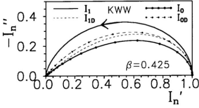
Figure 1. Complex plane plots of exact, normalized KWW frequency response. Curves I1 and I0 illustrate direct
KWW1 and KWW0 complex resistivity response (solid lines), and I
1D and I
0D show corresponding curves
calcu-lated by transforming the KWW data to the complex dielec-tric constant level and subtracting dc conductivity eects (dashed lines). The arrow shows the direction of increasing frequency.
Figure 1 presents complex plane plots ofI nfor
n= 0 and 1, results which demonstrate some of the dierences between exact KWW0 and the corresponding KWW1 model response. Because of the presence of the x -factor inG
1(
x), it yields response much closer to single-relaxation-timeDebye response than does KWW0 when
1 =
0, the present choice. Now when -level data (calculated as in Eq. (11) with
C1 = 0 using the KWWn form of G
n(
x)) are transformed to the complex"level, one can represent the results using Eq. (12). Then it is straightforward to use LEVM to remove the eects of"
D 1and
D ofrom the data in or-der to obtain the eective I
D response associated with
the original CSD data. To do so, we use the value of
Cn=
C0n employed in generating the data, calcu-late
D 0 = 1 =
C0nand set the "
D 1 in Eq. (12) equal to the value of "
C1n calculated using Eq. (5), when the original(!) data were generated with"
C1= 0 :It turns out that"
C10 is zero for data involving a DCRT without high-frequency cuto, but not"
C11. Because the data were originally of CSD type, the resulting I
D curves are denoted byI
1Dand I
0D. It is surprising that although theI
1and I
0curves are so dierent, those for I
1Dand I
0D are quite similar.
III Direct data tting
A. CSD-typ edata
We shall start with exact synthetic CSD1 KWWl data generated using Eq. (11), with I
1(
!) set equal to the KWW1 model, and with parameter values the same as or close to those obtained with earlier KWW1 tting of actual 321 K Na2O-3SiO2data with electrode eects eliminated [4,23]. The resulting CSD1 param-eters are
C01 = 1
:4510
9 -cm,
01 = 0
:001s, and
1 = 0
:425: No
1 value was initially included, and
C1 was taken zero, in accordance with the results of earlier ts of the original data. The above values led to <x
,1 >
1
'0:3526,<x> 1
'12:91, C01
'100:57, and
C11
'22:09, using Eqs. (4) through (8). These KWW1 values are summarized in row A of Table 1, where
C0
(
C01)
,1. In this table S
F is the rela-tive standard deviation of a t, the standard deviation of the relative residuals. The synthetic data extended over the range 0:01!10
10radians/s with 10 points per decade evenly spaced on a logarithmic scale. All the complex-nonlinear-least-squares ts of lines B, C, E, and F, and the ts discussed later, involved propor-tional weighting and used the LEVM V. 7.1 program [27].
Next, the complex--level data of line A were trans-formed to the complex dielectric constant level, as de-noted by the designation KWWlD in row B. The t results of lines B, C, E, and F were obtained using Eq. (12). Here, all the values shown in these lines are di-rect t estimates with very small relative standard de-viations (not shown). The I
D(
has been conventional to use the symbolfor the frac-tional exponent parameter of the EDRT model [2,17], for simplicity it will be denoted by herein for easy comparison with KWW parameters.
Comparison of the results of lines B and C shows that the EDRT model provided a much better t of the CSD data at the dielectric-constant level than did the KWW model. Further, except for the expected dier-ence [2,4,23] between the
01value of line A and the
0D value of line C, one sees that the line-C estimated pa-rameter values are in excellent agreement with the ex-act ones of line A, and, specically, that the
D 0 value of line C is an exceptionally close estimate of 1=
C01. Thus, although the
D 1values of lines B and C are de-noted by a subscriptn=Dto indicate their estimation at the dielectric level by a complex-dielectric- constant response model, we see that they are, in fact,
C1 es-timates, necessary here because no actual DSD
D 1 values have been included, and we are dealing solely with CSD-type data, not DSD.
Usually, additional information will be required to distinguish between a true DSD data set and its trans-form tted by a CSD approach, or, conversely, between a true CSD data set, and its transform tted by a DSD approach. Nevertheless, we shall, for convenience, des-ignate DSD data tted by a CSD approach, as in Eq. (11), by CSD designations, and CSD data tted by a DSD approach, as in Eq. (12), by the DSD designation. Finally, synthetic data like that of line A were gen-erated with a permittivity
V
Sin series with the rest of the response. Here the series dielectric constant
S = 10 is used to represent the eect of the capacitance of com-pletely blocking electrodes. The value of 6.884 in line D is just the series combination of 22.09 and 10, and (
D 1+
D) should equal 10, as it does for line D. Here we see from lines E and F that although the -K model leads to a better t than does the -E one, contrary to the results in lines B and C, both ts are relatively poor and are much worse than that of line C.
It is interesting that because of the presence of S it is unnecessary to include a
D 0 dc conductivity in the t models of lines E and F, unlike the situation for lines B and C. When either
S or
D 0is taken as a free parameter of the t at the dielectric level, the initial values progressively change until neither one makes any contribution to the t. Thus, while each can be accu-rately estimated from CSD1 tting of the data, neither can be estimated by tting at the dielectric level using Eq. (12)! For actual experimental data, if the presence
of complete blocking were unrecognized, one might well conclude that dielectric-level data similar to that used to obtain the t results of lines E and F were those of a pure dispersed dielectric material (true DSD response) without any dc resistive leakage. Here we know that it is not, and it is worth emphasizing that instead of the 3%S
F of the t of line E, transformation of the data to the complexor M level and its tting with the ap-propriate CSD model, here the KWW1, as in line D of Table 1, yields an exact t.
Although a zero value of
D 1 was used in gener-ating the CSD data of rows A and D, if a non-zero value had been included, as is always necessary for the analysis of experimental data, we would have found that the \
D 1" estimate in lines B and C should have been designated as
1 and would have included
D 1 since tting of this kind can only yield estimates of
1
C1+
D 1 [2,3,23]. Thus for actual CSD data, one can only estimate
D 1directly from a CSD t and then calculate
C1and
C0from such t results. In the absence of any DSD in the measured frequency range, one can take the actual, always present,
D 1 equal to
D 0, and we must identify the apparent DSD and non-zero
Das arising solely from CSD. Finally, it is worth remarking that an EDRT response model was found most appropriate for tting dispersion results for the conductive material CaTiO3:30%Al
3+at low tempera-tures using DSD tting at the dielectric level, as in row C of the present Table 1 [18]. The synthetic-data results of lines B and C perhaps suggest why a EDRT model was there found to yield a closer t of the experimental data than the KWWD model.
B. DSD-type data
Let us now regard the best-t EDRT results of row C of Table 1 as representing possible DSD response with non-negligible leakage resistance. For concreteness, the parameter estimates and EDRT response model of row C were used to generate a new exact data set. The data were then transformed to the complex resistivity level and tted with Eq. (11) using several models, all with
C1 = 0. The best-t model found, was, not surpris-ingly, the KWW. Since leakage resistance can be of any value, in order to investigate its eects three dierent values of the dc conductivity,
0=
D 0, are used in col-umn 7 for lines A, D, and G of Table 2. That for line A is the value shown in row C of Table 1, designated as
C0 1=
C01= (
C1)
Finally, all three of these sets of exact data implicitly involved
D 1 = 10, obtained by setting
1 = 32 :11
rather than the 22.11 of row C of Table 1.
TABLE 1. DSD tting results of exact CSD data calculated using Eq. (11) with the KWW1 model and the parameter values of rows A and D. These data sets were t at the complex dielectric constant level using Eq. (12). Here
S is the dielectric constant of a series capacitance, and -K and -E designate the use in this equation of the KWWD model or the EDRT model, respectively. The presence of a non-zero value of
S changes the interpretation of the
n1 and
nquantities, as discussed in the text.
n1 equals either
D 1 or
C11 as appropriate. S
F is the relative standard deviation of a t.
TABLE 2. CSD tting results of exact DSD data calculated using Eq. (12) with the EDRT model, the parameter values of rows A, D, and G, and
D = 78.48. These data sets were t at the complex resistivity level using Eq. (11) with a KWW1 or KWW0 model, and a parallel conductivity,
CP. For the KWW0 ts, the
D 1-column values are actually those of
1=
C1n+
D 1. The dimensions of the
's and of 1=
Cnare (-cm)
,1. Here
0 is the total dc conductivity.
Comparison of the results shown in lines A of Ta-ble 1 and B of TaTa-ble 2 shows that the EDRT model represents the original data at the dielectric level very well since the CSD t results of line B are very close to the exact ones of Table 1, line A, completing the circle of transformations and ts. The numbers shown in the
CP column of Table 2 are values of a
paral-lel conductivity parameter included in the KWW1 ts. Non-zero values are required in order to obtain a good estimate of the total dc conductivity,
0=
CP+
C0, when
C0
6
=
D 0. This is because the CSD constitutive equations, (5-8), hold for Eq. (11) ts, as indicated by the row-E t of Table 2. As we see, the
quan-tity even when the total dc resistivity is very dierent. Incidentally, in those situations where a non-zero value of
CP was required, taking
C1 as a free tting pa-rameter instead of
CPled to completely unsatisfactory ts.
Although the KWW0 t of line C is slightly better than the KWW1 one of line B, it requires a non-zero value of
CP, and, without it, the resulting S
F had the much larger value of 0.024. Further, since the original KWW1 data included no
CP, the non-zero KWW0
CP value is anomalous and helps one decide whether a KWW0 or KWW1 t is more appropriate for CSD data, where one usually expects to nd
CP = 0. Com-parison of the values shown in lines B and C, E and F, and H and I indicate, nevertheless, that the relation
0+
1= 1, proposed earlier [3,23], is closely obeyed. The results in the table show that when the esti-mated value of
CP is non-zero, the estimated parame-ter values in lines E and H are not as close to the ones used to generate the original KWW1 data as when it is zero, but the parameter values are still relatively close to the original exact-data values, and the CSD-t values of
0are good estimates of the proper dc conductivity. These results provide further useful discrimination in-formation. For experimental CSD response, good ts of the data are nearly always found without the need to include a parallel
CP tting parameter, and negative estimates of this quantity are physically unlikely for a passive system. Thus, the presence of a signicant non-zero CSD1 DCRT- model tting estimate of
CP is an excellent indication that one is not dealing with ordi-nary CSD response but probably with leaky dielectric dispersion.
The small but non-zero S
F = 0.0071 value in row B of Table 2 is an indication that the KWW1 CSD1 tting model, I
1(
!), is not quite entirely appropriate forI
D(
!) EDRT DSD data, and it is reasonable to as-sume that if an appropriate model were available, an exact t would be found. For actual experimental data, where the errors present in the data generally lead to S
F values greater than 0.0071, the distinction is usually unimportant.
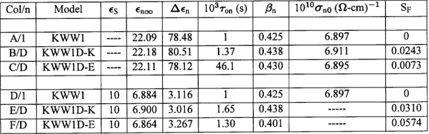
Figure 2 compares theM"(!) curves for the ts of lines B, E, and H of Table 2 and for two smaller val-ues of the dc conductivity. Particularly interesting is the double-peak curve present when
0is smaller than
C0. No trace of such behavior is apparent for any of the corresponding {"(!) curves. Because the line-H t is the worst of the three, both the original data and the
t points are included, but only the data lines or points are presented for the other curves. Estimation of the DRTs associated with these cases can shed further light on their dierences and is explored in the next section. When two peaks are present, the peak of the lower-frequency one appears at lower and lower frequencies as
0 decreases, as illustrated by the curve with
r= 0:01. Finally, when there is no dc conductivity, this response disappears from the measurable frequency range.
Figure 2. Comparison of the threeM"(!) data-line curves
for rows A, D, and G of Table 2, and t points for row H (open circles), and, as well, curves for two other smaller xed values of
0. Here
r
0 =
0A where
0A =
C0 =
6:89510
,10 (-cm),1 is the dc conductivity included in
the original exact EDRT dielectric data for row A of Table 2, and the rst three0values are those of rows D, A, and
G of column 7 of Table 2.
N = 1 s here and elsewhere.
IV Data inversion and
identi-cation of dispersion types
A. Background
Gross [5,7-9], Gross and Pelzer [6], and Kita [28] have been concerned with deriving analytic integral transforms connecting the DRTs associated with the I
1(
!) and I D(
involving inversion is illustrated, one which yields DRT estimates which represent their associated frequency re-sponse with extremely high accuracy and do not require analytic expressions.
For the KWW model in the small-x region, the G
0( x) orG
D(
x) DRT is proportional tox
,(1,n)and so diverges in the limit for
0 or
D
<1 [2,29,30]. There-fore, it is more instructive to plot F
D
; which does not diverge in the limit, vs. yor log(x), rather than to plot G
D(
x) vs. log(x). The above denitions and analysis show that for the KWW and other similar modelsF
D andG
1are proportional to xG
Dand xG
0 respectively, and do not diverge as x!0. For direct comparison of inversion results that estimateG
0 and G
1, or G
D and G
1 from the same frequency-response data, it is most useful to compare the normalized distribution estimates ofF
0or F
Dand G
1. For accurate inversions, F
0and G
1 should be identical. The LEVM program estimatesF
1 directly for CSD1 analysis, but then outputs the corre-spondingG
1while CSD0 or DSD inversion yields F
0or F
D. For convenience, let
H(x) denoteF D,
F 0, or
G 1. The high-resolution numerical inversion algorithm in the LEVM program yields a total of M points of a continuous, discrete, or mixed distribution, whereM is presently limited to a maximum of 19. Therefore, for such results, we replace H(x) by H
i, with 1
i19. LEVM inversion yields estimates of theM point pairs, fH
i ;x
i
g, where both quantities are free variables of the t [11], not the case for other inversion techniques. Dis-crete and continuous-distribution points may therefore be unambiguously identied by comparing results for two dierent values ofM [11]. For continuous distribu-tions, allx
iestimates will be dierent for the two inver-sions, but the x
i values of any discrete points present will remain the same. In the LEVM inversion algo-rithm, which uses numerical quadrature, it has not been found possible to account for end-point eects accu-rately for arbitrary distributions. Therefore, those H
i estimates with the smallest, and sometimes largest x
i values, and, to a lesser degree, their immediate near-est neighbors, will be less accurate than the remaining estimated points of the inversion [4,11,30].
In the preceding section, we have shown by tting of accurate numerical data that there is a very close con-nection between an EDRT representing a distribution of \dielectric" relaxation times and the corresponding KWW1 DRT representing a distribution of \resistiv-ity" relaxation times: data generated by one of these response functions may be closely t when the other is
used instead, as demonstrated by the results presented in Tables 1 and 2. This connection has been further investigated by inversion, and some of the results ob-tained are presented in Figs. 3 through 5.
B. DRT inversion estimates: Fig. 3
re-sults
To obtain the DRT results shown in Fig. 3, CSD1-type KWW1 frequency response data were produced using the parameters of row A of Table 1, except that
D 1 was usually taken as 10 rather than zero, yield-ing
1
'32:09. The 1,AF
D distribution-of-dielectric-relaxation- times curve shown in Fig. 3 was obtained by numerically inverting this data set, expressed at the complex dielectric constant level, using Eqs. (1) and (12). For comparison, the 2,A data for inversion in-volved the parameters obtained from a t of the 1,A data using the EDRT model. The close agreement be-tween the 1,A and 2,A curves again shows that the EDRT is a good approximation to the distribution of \dielectric" relaxation times associated directly with the original KWW1 data. Because of inaccuracies in the largest- points of the two curves, it is dicult to isolate any signicant dierence between them, al-though an accurate EDRT should yield a straight line until the appearance of an abrupt cuto near =
0 = 1. [17,30]. These inversions included the free parame-ters
1 and
0 as part of the full tting circuit and led to estimated values of them in virtually perfect agreement with those expected. No adequate inversions could be obtained without the inclusion of these param-eters since they contributed appreciably to the full data which were inverted. The errors in all the smallest- points for the various curves are clearly evident in this gure.
The points of theG
1DRT curve marked
1,A;CSD in Fig. 3 have been tted directly to the KWW0 dis-tribution using LEVM. Such tting yields estimates of
1and
01. The S
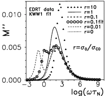
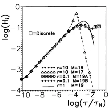
Figure 3. Log-log plots of H; DRT strengths vs. . In
the legend, indicates dielectric-level inversion to estimate
dielectric DRTs, whileindicates resistivity-level inversion
to estimate the related distributions of resistivity relaxation times. Here 1,A and 2,A denote data associated with the A-row of Tables 1 and 2, and CO identies a cuto distribu-tion withymin=,10.
D 1was 10, except where indicated
otherwise.
It is important to note that the 1,A;CSD and 2,A;CSD results represent basic distributions which do not include the eect of any non-zero
D 1. One obtains exactly the same results inverting data with
D 1= 0 or data with
D 1
6
= 0, provided that the eect of non-zero
D 1 is properly included in the inversion procedure. Unfortunately, unlike the inversion of data to obtain a distribution of dielectric relaxation times, as discussed above, inversion to obtain a distribution of resistive re-laxation times does not allow a quantity such as
D 1to be a free parameter, thus it cannot be estimated from the inversion t but must rst be estimated as in the ts of 1,B or 1,C and then taken as a xed parameter in the CSD inversion.
The curves in Fig. 3 with
D 1 = {1O and + 20 show the eect of not accounting for a non-zero
D 1in the inversion. As demonstrated, when
1
< (>) C1 the apparent DRT is wider (narrower) than the proper KWW0 distribution and is not well tted by such a distribution. When
D 1 is of the order of 100 and is not accounted for in the inversion, the resulting distri-bution shows a straight-line portion very close to that of the 2,A EDRT one.
Direct tting to the KWW0 distribution model of the 2,A;CSD results with end points omitted led to
S F
' 0:02, with parameter estimates equal to those of the original KWW1 model to nearly three signi-cant gures. Thus, although the KWW DRT is not quite the exact CSD distribution related to the DSD EDRT, comparison of the relevant curves in the gure shows that any dierence is virtually imperceptible in a log-log plot and suggests that for usual experimental data containing only random errors it would be dicult to verify any dierence. Incidentally, although CSD0-type inversion of the 2,A EDRT data was carried out, it did not lead to a DRT close to that of the KWW0 but instead to one nearer in form to the original EDRT of curve 2,A.
Meixner [31], and later Gross [5,8,9], stated that if one of a continuous-distribution DRT pair was trun-cated within a limited interval, then the other distribu-tion of the pair would be continuous in the same interval and be zero outside, except for the appearance of a sin-gle discrete line. Later, Gross [9] presciently pointed out that such lines need not always appear, but he did not explicitly specify the general conditions required for their appearance or absence. Here, we do so be-low. Incidentally, Gross [9] made the cogent comments that (a) either, but not both, of related Maxwell and Wagner-Voigt models can have physical signicance for a given real material, and (b) the discrete lines which sometimes appear have hardly more than mathemati-cal signicance. An important purpose of the present work is to nd clues from tting and inversion which may allow one to decide which one of the DRTs in (a) is associated with a physically signicant model.
The two curves marked \CO" in Fig. 3 are ones in which the EDRT used in generating the data was cut o by using ymin = ,10: Now since log(min=
N) = l og f0
Dexp( ymin)=
N
g with
N = 1 s, the result is about {5.68. The points with smallest on the two CO curves are both at about {5.60. As theM value used in the inversion increases, the smallest- value found decreases toward the cuto limit. The two DRTs are clearly non-zero over the same interval, as required by the earlier work, but no discrete line is found for the distribution of resistive relaxation times, contrary to the earlier predictions. Incidentally, the S
F values of LEVM inversion ts of the present type decrease sub-stantially for exact data asi!i+ 1 and as the width of the non-zero interval of a continuous distribution de-creases. For example, typical inversions such as the 2,A; CSD one of Fig. 3, where M = 19, have S
values of about 310
,4, while the CO curves with M = 13 lead to S
F values less than 10
,5. These re-sults show how closely the inversion-t models t the original frequency-response data and make it clear that with such good ts there is no possibility of missing a discrete line.
C. DRT inversion estimates: Fig. 4
re-sults
We have seen that while changes in
D 1change the shape of the DRT obtained by inversion of the full data when the presence of
D 1 is unaccounted for, no dis-crete line occurs. But since changes in
D 1 do not di-rectly involve the CSD constitutive equations, Eqs. (5-8), it is worthwhile investigating the eects of changes which do so. Some inversion results, with all non-zero
D 1 eects properly accounted for, are presented in Fig. 4 for the three dierent values of
0used in rows A, D, and G of Table 2. Dene r as the ratio of the xed
0 values of rows D or G of column 7 of Table 2 to the xed
0=
C0value listed in row A. The r= 10 and r = 0:1, M = 19A curves are inversion results obtained with no
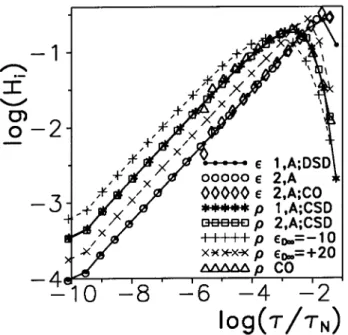
CP parameter included in the inver-sion; thus they should not be expected to yield proper DRT estimates.
The two r= 10 curves demonstrate that changing M does not signicantly change the optimized value of the peak point, thus suggesting that this point arises from a discrete line while the other points are associated with a continuous distribution. Similarly, appreciable changes inM for the rstr= 0.1 curve do not change the position of the circular-symbol point enclosed in the square, thus verifying that this point also represents a single discrete DRT.
Suppose that we now account for the need for a non-zero
CP by including such a separate, parallel conduc-tivity parameter in the full inversion model. For the r= 10 results, one nds, as expected, that the inclusion of such a parameter with a xed value of 69:0210
,10 (-cm),1 results in a DRT estimate in full agreement with that designated by 2,A; CSD in Fig. 3. Here that curve is reproduced as the solid line labeledr= 1, M = 19 and is shown without any points included. Thus, no discrete line appears when the eect of
CP is properly taken into account.
But what happens for the r = 0:1 situation when a negative
CP is included? Again one nds that the inversion points approach the usual CSD r = 1,
M = 19 distribution as
cpdecreases from zero toward the Table-2 row-H t value of,6:04610
,10(-cm),1. Inversion with a non-zero value of
cpnear that above is dicult because it involves the small dierence between two nearly equal large numbers. The points identied byr= 0:1,M = 19Bin the gure are the largest eight values found in the inversion when the parallel conduc-tivity used in the inversion was set to the intermediate value of ,1:710
,10(- cm),1. The other points of the 19 fell very closely on ther= 1 line. Here the last point on the right is still a discrete-distribution one, but we see that, as the added parallel conductivity be-comes more negative, all the higher- points approach ther= 1 line as the proper value of
CP is approached. For this value, the discrete point has disappeared and all points are those of the expected continuous distri-bution. The present results suggest that the presence of a discrete line in previous analytical calculations of a CSD DRT arose because the need for
CP was unrec-ognized and thus was not included in the analysis.
Figure 4. Inversion results similar to those of Fig. 3 except that the eects are demonstrated of three dierent choices for the conductivity ratio r dened in the Fig.-2 caption
and used in generating the data. All inversion results shown were carried out with the parallel conductivity, CP taken
zero except for theM = 19Bcurve, where
CP was xed at ,1:710
,10 (-cm),1. With the proper
CP values used
in the inversions (see Table 2), the r= 0:1 andr = 10
re-sults agreed with the KWW0-DRTr= 1 curve shown. All
D. DRT inversion estimates: Fig. 5
re-sults
Kita [28] was unable to obtain analytically a DCRT expression from a particular distribution of dielectric relaxation times, that of Davidson and Cole [DC] [32], which satised the principle of equivalence of Maxwell and Wagner circuits. See the Appendix for details about this important principle. Gross [8,9] showed that the principle was valid if the calculated Wagner-Voigt DRT included a discrete line, shown to arise from the intrinsic cuto (truncation) of the DC distribution at >0
D. Incidentally, Kita's work also suggests that the CSD response most appropriately associated with a Maxwell-model DSD data set is of CSD1 rather than CSD0 type.
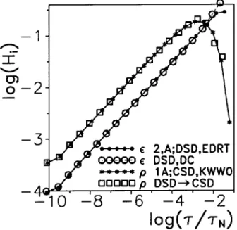
Figure 5. Inversion results for the dielectric DRTs (desig-nated with ): (a) the 2,A exponential DRT, EDRT,
re-peated from Fig.3, and (b) the Davidson-Cole DRT, DC. Also shown are CSD-inversion DRT estimates associated with (b), marked DSD !CSD, and the 1,A,CSD KWW0
DRT, also repeated from Fig.3, both designated with .
Since we have demonstrated earlier that abrupt cut-o cut-of an expcut-onential distributicut-on at a smallmin value does not lead to the appearance of a discrete line, it is worthwhile to apply the present methods to estimate points of a DDRT, starting with DC data at thelevel. First, however, for the convenience of the reader in com-paring the work of Gross and Kita, it is worth pointing out that Kita's symboldenotes the dielectric permit-tivity, here
V, while Gross [8] denes
as the com-plex dielectric constant but then omits a necessary
V term in his admittance and time-constant expressions.
For easy comparison, two DRT curves previously presented and discussed are included in Fig. 5. The curve marked DSD,DC is the distribution of dielectric relaxation times estimated by inversion of exact DC data. The original KWW1 frequency-response data were tted using the DC model (with a somewhat less accurate t found than that obtained with the EDRT model), and then exact DSD data were generated with the DC model using the values of the appropriate pa-rameters of Section III-A, except that 0
D was set to 0.025 s, the approximate t value. Comparison of the rst two curves identied in the gure indicates ex-tremely good agreement between the EDRT DRT es-timate and that for the DC situation except for the three highest- points. As expected, for the DC curve we see the approach to an innite value at cuto, but because of the problem with end-point estimates, the last two points do not rise as fast as required for an ex-act DC DRT. The maximum- estimate withM = 19 was about 0.021 s, and it was found to approach closer and closer to the cuto value of 0.025 s as the value of M used in the inversion was increased.
The last two curves in Fig. 5 compare the practi-cally exact KWW0F0, or, equivalently, the KWW1G1 distribution, with the CSD1 inversion estimate of G1 associated with the exact DSD DC data. We see that although the agreement is not quite as close as that for the comparable EDRT -level comparison of Fig. 3, the agreement is still suciently good that for typi-cal experimental data one would not be able to distin-guish well between the three dierent DRT estimates. Although tting comparisons for DDRT estimates ob-tained from the same data might allow somewhat bet-ter discrimination, the most appropriate tting model can be much better identied from direct tting in the frequency domain of original frequency-response data. The present results again conrm that accurate inver-sion estimates of truncated DSD DRTs need not lead to the appearance of a discrete response line.
V Summary and conclusions
mobile charges. This conclusion is foreshadowed by earlier work [3] in which it was demonstrated that the limiting high- and low-frequency log-log slopes of all immittance responses are exactly the same for DSD and CSD1 response when
1 =
D and for DSD and CSD0 response when
0 = 1 ,
D, provided the DSD response involved
0
6
= 0 and the CSD response in-volved
D 1
6
= 0:
Here, we nd that the requirement that CSD and DSD approaches (possibly involving conductive or di-electric distributions of relaxation times, respectively) be able to t data equally well necessitates an augmen-tation of the Wagner-Voigt relaxation circuit usually considered in applying the principle of equivalence of Maxwell and Wagner-Voigt circuits. CSD model re-sponse, Eq. (11), involving a discrete or continuous dis-tribution of conductive relaxation times in the Wagner-Voigt circuit, must not only be augmented by the ef-fects of a parallel specic susceptance (associated with the limiting dielectric constant
D 1) [2,3,23], but also by a parallel conductivity, here designated as
CP. See the results presented in Table 2. In exceptional cases,
CP, which is not a separate parameter in DSD tting, must be negative to allow adequate CSD tting of arbi-trary DSD data. When a
CP estimate is negative, it is highly unlikely that the response of the physical system investigated is dominated by dispersion associated with mobile charges, rather than by purely dielectric eects, and it is still unlikely even when
CP is positive and signicant compared to
0. Thus, though discrimina-tion is not unambiguously possible when
CP
6
= 0, it is nevertheless plausible. Conversely, when an estimate of
CP is statistically indistinguishable from zero, the data may, in principle, be equally well tted by a CSD or a DSD approach, thus precluding discrimination us-ing only a sus-ingle data set.
The present analysis leads to the important conclu-sion that if CSD data involves KWW1 I
1(
!) disper-sive response, then the EDRTI
D(
!) response model is an appropriate choice for DSD tting of the data using
Eq. (12). Although the use of the Davidson-ColeI D(
!) model for generating DSD data also leads rather closely to KWW1 CSD response, somewhat better results are found for the KWW1, EDRT pair.
The prediction [8,9,31] that truncating a full-range DSD DRT, or using the DC, which involves an intrin-sically truncated distribution, leads to CSD response with both a continuous DRT and a discrete response line has not been veried by the present work. It has, however, been found that when
CP is not accounted for in the inversion, such a line appears whether the original DSD DDRT is truncated or not. When inver-sion of frequency-reponse data is used to estimate a CSD DCRT, taking proper account in the tting pro-cedure of non-zero
D 1 and
CP parameters allows one to obtain an accurate estimate of the true continu-ous DRT involved, but omission of such parameters in the inversion leads to erroneous estimates, as shown in Figs. 3 and 4. None of the earlier analytical DRT work [8,9,28,31] took explicit account of these parameters, possibly explaining the present discrepancies.
Although DSD and CSD inversion results are in-structive and can be useful for distinguishing between continuous and discrete parts of a DRT, it appears that direct tting of frequency- (or temporal- [2,25]) response data is likely to allow better discrimination between various possible dispersive models for DSD or CSD tting, and, in some cases, it can lead to a plausi-ble conclusion about the identity of the dominant phys-ical processes involved in the dispersion. Measurements over a range of temperatures should allow even better decisions about the character of the dominant disper-sion process to be reached.
Acknowledgment
Denition of Acronyms
ac Alternating current
CSD Conductive-system dispersion
CSDn n = 0 or 1; see below for denitions of the n values dc Direct current
DC Davidson-Cole response model
DCRT Distribution of conductive-system relaxation times DDRT Distribution of dielectric-system relaxation times DRT Distribution of relaxation times
DSD Dielectric-system dispersion
EDRT Exponential distribution of relaxation times KWW Kohlrausch-Williams-Watts response model
KWWn KWW response dened by index n, where n = D, 0, or 1 (see below) LEVM The complex-nonlinear-least-squares tting program used herein n=D The response is of DSD character involving a DDRT
n=C The response is of CSD character involving a DCRT and n = 0 or 1 n=0 The response is of CSDO character, possibly involving a DCRT formally
equivalent to a given DDRT
n=1 The response is of CSDl character involving a DCRT related to a given CSDO DCRT by Eq. (13) of the text
APPENDIX
Because of the importance of the principle of equiva-lence for relaxation systems, it is worthwhile to summa-rize some historical information about it, most of which appears in Ref. 33. Two two-terminal passive circuits with time-invariant elements are said to be equivalent when their responses over the full frequency range are exactly the same. Consider pure reactance circuits rst, ones made up only of non-dissipative ideal capacitative and inductive elements. In 1924 Foster [34] proved that any such reactance system can be equivalently repre-sented by a parallel combination of resonant elements (capacitance and inductance in series) or by a series combination of antiresonant elements (capacitance and inductance in parallel). To account properly for pole and zero behavior at zero and innite frequencies, sin-gle elements must also be included in order to obtain full equivalence [35].
Later, Bode [36] showed that the Foster reac-tance theorem could be generalized by a frequency-transformation method. For a relaxation situation, his procedure replaces inductances in the original re-actance system by resistances. This procedure can thus lead to Maxwell and Wagner-Voigt circuits which are equivalent. As shown herein, for full equivalence of dielectric- system response to conductive-system re-sponse (in which the eective resistance at innite fre-quency associated with the dispersion process is zero), the Maxwell circuit must, in general, include a capaci-tor and a resiscapaci-tor in parallel with the rest of the circuit,
and the Wagner-Voigt circuit must also include such parallel elements. The parallel capacitance represents the high- frequency-limiting dielectric constant of the system, and the parallel resistances are dierent for the two cases. Actual transformations from one circuit to the other are best carried out by complex-nonlinear-least-squares tting [27], but Novoseleskii et. al. [37] have provided some useful analytical expressions for do-ing so for circuits with only three or four elements. The present work demonstrates that the principle of equiv-alence applies for continuous distributions as well.
References
1. J. R. Macdonald, J. Appl. Phys. 58, 1955 (1985). 2. J. R. Macdonald, J. Non-Cryst. Solids 197, 83
(1996); erratum: ibid204, 309 (1996), andG Din Eq. (A2) should beG
CD, the present G
1quantity. 3. J. R. Macdonald, J. Appl. Phys. 82, 3962 (1997). 4. J. R. Macdonald, inElectrically Based Microstruc-tural Characterization, Proceedings, p. 71, Vol. 411, Fall meeting, November 1995, Boston, MA (Materials Research Society, Pittsburgh, PA, 1996).
5. B. Gross, J. Appl. Phys. 18, 212 (1947);ibid19, 257 (1948),ibid62, 2763 (1987).
6. B. Gross and H. Pelzer, J. Appl. Phys. 22, 1035 (1951).
7. B. Gross, Mathematical Structure of the Theories of Viscoelasticity(Hermann & Cie, Paris, France, 1953).
10. J. R. Macdonald and C. A. Barlow, Jr., Rev. Mod. Phys. 35, 940 (1963).
11. J. R. Macdonald, J. Chem. Phys. 102, 6241 (1995); Computers in Physics9, 546 (1995). 12. A. R. Long, Adv. Phys. 31, 553 (1982).
13. J. R. Macdonald, J. Appl. Phys. 62, R51 (1987). 14. S. R. Elliott, Adv. in Phys. 36, 135 (1987). 15. S. R. Elliott, Solid State Ionics70&71, 27 (1994). 16. J. R. Macdonald, Phys. Rev. B 49, 9428
(1994-II).
17. J. R. Macdonald and J. C. Wang, Solid State Ion-ics60, 319 (1993).
18. J. R. Macdonald, J. Non-Cryst. Solids 210, 70 (1997).
19. S. R. Elliott, Phil. Mag. 36, 1291 (1977). 20. A. K. Jonscher, Dielectric Relaxation in Solids
(Chelsea Dielectric, London, 1983).
21. L. A. Dissado and R. M. Hill, J. Chem. Soc. Fara-day Trans. 280, 291 (1984).
22. J. C. Giuntini, J. V. Zanchetta, and F. Henn, Solid State Ionics28-30, 142 (1988).
23. J. R. Macdonald, J. Non-Cryst. Solids 212, 95 (1997). The symbol
0 should be removed from the right end of Eq. (12); Eq. (7) in this work does not apply to Eqs. (3) and (4) when
C1
6
= 0 (see Ref. 2, above); and the word \frequency" in the third line from the bottom of the seconf col-umn of p.111 should be \temperature".
24. J. R. Macdonald, J. Chem. Phys. 36, 345 (1962). 25. J. R. Macdonald, J. Appl. Phys. 84, 812 (1998). The word \out" in the third line from the bottom of the rst column on p.820 should be \but". 26. R. Kohlrausch, Pogg. Ann. der Phys. und
Chemie, (2) 91, 179 (1854); G. Williams and D.
C. Watts, Trans. Faraday Soc. 66, 80 (1970), G. Williams, D. C. Watts, S. B. Dev, and A. M. North, Trans. Faraday Soc. 67, 1323 (1971). 27. J. R. Macdonald and L. D. Potter, Jr., Solid
State Ionics 23, 61 (1987). The latest ver-sion of the LEVM tting program, V. 7.1, may be obtained at no cost from Solartron Instru-ments, Victoria Road, Farnborough, Hampshire, GU147PW, England; e-mail, attention Mary Cut-ler, lab,[email protected]. More details about the program appear in
http://www.physics.unc.edu/macd/. 28. Y. Kita, J. Appl. Phys. 55, 3747 (1984).
29. E. W. Montroll and J. T. Bendler, J. Stat. Physics 14, 129 (1984).
30. B. A. Boukamp and J. R. Macdonald, Solid State Ionics74, 85 (1994).
31. J. Meixner, Kolloid Z.134, 3 (1953).
32. D. W. Davidson and R. H. Cole, J. Chem. Phys. 19, 1484 (1951).
33. B. Gross and M. T. de Figueiredo, J. Appl. Phys. D18, 617 (1985).
34. R. M. Foster, Bell Syst. Tech. J. April, 259 (1924).
35. H. W. Bode,Network Analysis and Feedback Am-plier Design (New York, Van Nostrand, 1945), pp. 181-182.
36. H. W. Bode,Network Analysis and Feedback Am-plier Design (New York, Van Nostrand, 1945), pp. 214-215.