doi: 10.1590/0101-7438.2016.036.03.0421
MODELING AND SOLVING A RICH VEHICLE ROUTING PROBLEM FOR THE DELIVERY OF GOODS IN URBAN AREAS
Jos´e Ferreira de Souza Neto and Vit´oria Pureza*
Received June 10, 2015 / Accepted October 25, 2016
ABSTRACT.This work addresses a vehicle routing problem that aims at representing delivery operations of large volumes of products in dense urban areas. Inspired by a case study in a drinks producer and dis-tributor, we propose a mathematical programming model and solution approaches that take into account costs with own and chartered vehicles, multiple deliverymen, time windows in customers, compatibility of vehicles and customers, time limitations for the circulation of large vehicles in city centers and multiple daily trips. Results with instances based on real data provided by the company highlight the potential of applicability of some of the proposed methods.
Keywords: city logistics, vehicle routing problem, time windows, multiple deliverymen, multiple trips.
1 INTRODUCTION
Vehicle routing problems arise in many practical situations, including the delivery of goods to customers, the pick-up and the transportation of urban waste to regulated landfills, the elabora-tion of itineraries for electrical vehicles with stops in recharging staelabora-tions, the transportaelabora-tion of people with reduced mobility, and equipment repair in different houses. The literature presents several surveys on problem variants, solution methods and real applications, such as Bodin et al. (1983), Assad (1988), Ronen (1988), Osman (1993), Desroisiers et al. (1995), Cunha (2000), Breedam (2001), Br¨aysy & Gendreau (2005a, 2005b), Parragh et al. (2008), Laporte (2009), Bal-dacci et al. (2010), Belfiore & Yoshizaki (2013) and Schneider et al. (2014). The large number of contributions shows that a great deal of effort has been made for over 50 years by the scientific community when tackling these problems. This is due not only to their practical relevance but also to the difficulties faced when solving them. Nevertheless, as each studied case can present distinct features from what has already been discussed in the literature, new variations of the general problem continue to appear and require differentiated treatments.
*Corresponding author.
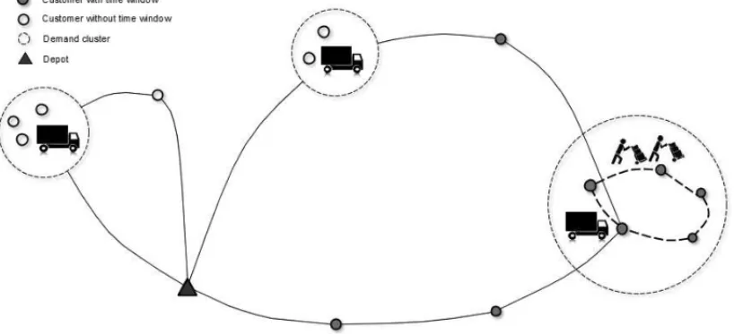
In this paper, we consider a variant that represents the situation of many companies that deliver large quantities of goods in highly dense urban areas in a daily basis. Given the difficulties in driving and parking, customers close to each other are clustered, and for each cluster, a single parking slot is used by the vehicle assigned to serve those customers. The deliveries are then performed on foot by the vehicles’ crew from the parking slot. The relatively long service times in each cluster when compared to the vehicles traveling times justify the use of multiple deliv-erymen as it allows the reduction of the time required by a single deliveryman to serve a cluster and consequently increases the number of customers visited during working hours. Avoiding the violation of working hours is a primary objective of such companies given its direct impact on overtime costs.
Situations such as the one described are common in Brazilian drinks and tobacco companies, for which a large number of customers consists of small and medium sized retailers located in urban areas. In addition to the traditional routing and scheduling decisions, the route plan must elect the crew size in each vehicle as service times depend on the number of deliverymen employed. Time windows for the deliveries are often present since they avoid conflicts in critical hours (for example, lunch time in restaurants) or with the deliveries from other suppliers. In addition, due to large demands or constraints that impede some customers from being visited by large vehicles, it is often necessary that one or more vehicles make a second tour (trip) from the depot (warehouse) to serve additional customers. The problem can therefore be referred as a Multi-trip Vehicle Routing Problem with Time Windows and Multiple Deliverymen (MTVRPTWMD).
The concept of routes with multiple trips for each vehicle was first addressed for the VRP in the working paper by Fleischmann (1990). The author propose an extension of the Clark & Wright (1964) savings heuristic to generate trips and use a heuristic for the bin packing problem to assign the trips to a homogeneous fleet. As pointed out in Petch & Salhi (2004), enabling multi-ple trips can be essential for tactical and strategic planning, allowing savings in all transportation costs. Since the introduction of the concept, several papers explore heuristic solution approaches such as tabu search (Taillard et al., 1996; Brand˜ao & Mercer, 1997; Olivera & Viera, 2007; Alonso et al., 2008; Seixas & Mendes, 2013), genetic algorithms (Salhi & Petch, 2007), and exact algorithms (Azi et al., 2010).
Our research, on the other hand, is inspired by the urban delivery operations of a drinks manu-facturer and distributor located in the state of S˜ao Paulo, Brazil. The delivery is carried out by multiple deliverymen in each vehicle (truck) and the logistic operation considers different char-acteristics and additional constraints from the models of the previous works, such as a limited heterogeneous fleet, the use of chartered trucks, multiple trips for the same truck, varying number of deliverymen in each trip, the existence of dangerous routes, limitations on circulation times of truck types in city centers and incompatibility of truck types and customers.
Delivery operations in urban areas are often difficult to implement due to several real-life con-straints. The consideration of multiple deliverymen and multiple trips adds more complexity to the problem, therefore, well-structured procedures capable to provide efficient solutions is of great interest to distributors. As far as we know, the decision on the number of deliverymen has not been explored in current computational systems designed to support vehicle routing and scheduling decisions. Nevertheless, its practical and theoretical relevance is highlighted in the taxonomy of routing problems, recently proposed in Braekers et al. (2015).
In addition to this motivation, in the case of the company studied, the number of deliverymen in each truck is fixed. Therefore, it is interesting to verify whether setting the number of deliverymen based on the specificities of each trip can bring benefits, such as cost reduction, satisfaction of constraints formerly violated, and the increase of the number of demand clusters visited within the deliverymen working hours. The last advantage is particularly relevant and directly related to the first; in our study case, we observe that even with multiple deliverymen and multiple trips, meeting the daily demand usually require the use of overtime. As the company is typical of the drinks sector, the model and solution approaches proposed can be useful for other suppliers, as well as for companies from other sectors with similar distribution operations. Besides the practical motivation, vehicle routing problems with multiple deliverymen remain little explored, which means that its continuing study can represent contributions to the body of knowledge in combinatorial optimization and distribution logistics.
The remainder of this paper is organized as follows. Section 2 presents a brief description of the company and the relevant aspects of its distribution operations. The mathematical model is pre-sented in Section 3, while Section 4 describes a GRASP approach for solving instances based on real data provided by the company. Section 5 presents the results and analysis of computational experiments with the model, the heuristic and a hybrid approach, followed by conclusions and perspectives of future research in Section 6.
2 THE COMPANY’S DISTRIBUTION LOGISTICS
In 2014, the company’s fleet accounted a total of 222 trucks for product delivery. The fleet encompasses six types of trucks, characterized by different numbers of doors, weight and space capacities and functionalities. In particular, some truck types have mobile platforms that allow lifting the cargo to a higher ground. In addition to the own fleet, the company hires trucks for periods of the year during which the requirements of the demand exceeds the transportation capacity (e.g., school vacations and national holidays).
Nevertheless, even with the use of additional trucks, a second trip from the warehouse may be necessary for each available truck, not only to meet high demands but also as the result of regulations that restrain the use of certain types of trucks. One example is a municipal law, valid in most large Brazilian cities, that allows the circulation of large trucks in city centers only in early working hours (usually up to 9:00 or 10:00 a.m.). The company also prohibits the use of some of its largest trucks in city centers due to their riding difficulties when the traffic is intense. Other constraints include the compatibility between the truck type and the customer. For instance, most supermarkets and hypermarkets require trucks equipped with mobile platforms while retailers whose location can only be accessed through narrow streets must be served by smaller trucks. However, in order to perform a second trip, the truck capacity utilization must be equal or greater than a minimum percentage (usually 83%).
In addition to the driver, the standard crew in each truck comprises a second man and they both deliver the goods to the customers. However, if the cargo is addressed to areas controlled by drug gangs (called “dangerous routes” by the company), a security guard is added to the standard crew. It should be noted that the guard does not act as a deliveryman; his/her role is solely to ensure the security of the crew, the cargo and the truck. For the two-man crew, service times in each customer are estimated by the company as 5 minutes plus 20 seconds per product pack (in case of hypermarkets or supermarkets) or 30 seconds per product pack (other market segments).
routing software. In fact, the only recorded scheduling constraints on customers are time win-dows in restaurants. For this market segment, deliveries must occur at least two hours prior the opening hours (mostly 9:00 a.m.) in order to cool the products.
Figure 1– A two-trip two-echelon distribution route.
At the time of the study case, the major challenge faced by the company regarding their delivery operations was cost reduction. Since the Brazilian drinks market is highly competitive, the com-pany’s policy is to meet all daily requests on the same day, which often exceeds the deliverymen working hours. In these cases, instead of overtime payment, the company offers compensatory time off. However, if the banked time is not taken by the end of the current fiscal year, the em-ployees must be paid for the overtime hours in the beginning of the following year. In order to avoid these costs, the company wants to eliminate overtime while maintaining the service level provided to the customers.
3 PROBLEM DESCRIPTION AND MODELING
Formally, the problem tackled in this paper consists of planning daily routes for a fleet of het-erogeneous vehicles in order to deliver goods to customers in urban areas. The fleet departs (and returns) to the company’s warehouse and encompasses own and chartered vehicles. For each of these categories, distinct costs are applied; fuel and maintenance (variable) costs incur in own ve-hicles while the affreightment contract between the company and the autonomous truck owners prescribe only hiring (fixed) costs to the chartered vehicles.
deliverymen lunch time (i.e., no overtime is allowed). If a second trip is performed, the vehicle is reloaded at the warehouse.
Each node in a given route represents the warehouse or a demand node. A demand node is a single customer or a cluster of customers, and it is represented by the associated parking site. We assume that clusters were previously defined (either manually or by a clustering algorithm) in order to ensure a maximum radial distance between each costumer and the parking site, and that parking sites are in the exact location of the single customer or one of the customers in case of clusters.
In each trip, the total cargo must not exceed the vehicle capacity, and the crew size is limited to 3, the capacity of the vehicle’s cabin. The number of deliverymen in a vehicle can vary from the first to the second trip, since changes in the workload may require a different number of deliverymen. In case of dangerous routes, the maximum number of deliverymen reduces to 2 in order to accommodate the security guard. Customers served in a given route must be compatible to the type of vehicle. In addition, large vehicles are limited to ride in city centers in determined periods of day.
Given the aforementioned constraints, the route plan should otimize three objectives according to the following order of priority: (1) maximize the number of demand nodes served; (2) minimize the cost with own and chartered vehicles; and (3) minimize the number of deliverymen employed.
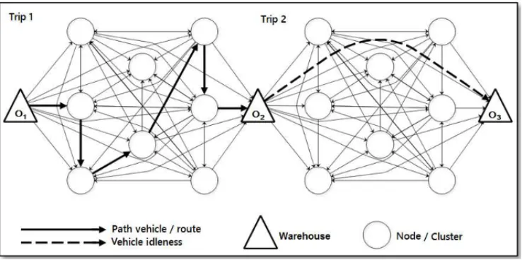
The problem combines characteristics of the VRPTWMD addressed in Pureza et al. (2012) and the MTVRPTW presented in Seixas & Mendes (2013), with several additional constraints. The flow network (Fig. 2) is represented by a graphG(n +2,A)with three types of nodes: n−1 demand nodes (represented by the associated parking sites) and three origins and/or destinations of the trips. Note that the warehouse is both origin and destination of trips, therefore, it is represented by the following three copies: nodes O1(origin of the first trip),O2(destination of the first trip and origin of the second trip) andO3(destination of the second trip).
Note that for modeling purposes, a route consists of exact two trips, which can represent three possible situations: (i) the vehicle idleness if the itinerary of the first and the second trip are
O1 → O2 andO2 → O3, respectively; (ii) a delivery trip followed by the vehicle idleness if the itinerary of the first trip is different fromO1 → O2and the itinerary of the second trip is
O2 → O3; and (iii) two delivery trips if the itinerary of both the first and the second trip are different fromO1→O2andO2→ O3, respectively. Figure 2 depicts situation (ii).
Consider the following notation:
• Indexes
i, j,h,m Demand nodes (represented by associated parking sites) and the ware-house copies. Ifi is a demand node, i = C1,C2, . . . ,Cn. If i is a warehouse copy theni =O1,O2,O3;
k,o Fleet(k,o=1, . . . ,K);
l,g Crew size assigned to a vehicle(l,g =1, . . . ,L). If the crew size isl, we say that the vehicle travels in model;
r Trips(r =1,2).
• Sets
C Demand nodes;
D Warehouse copies;
O W N Own fleet;
C H ART E R Chartered fleet;
B Demand nodes located in the city center;
A Demand nodes located in drug gangs areas;
E Vehicles with time circulation limitation in the city center;
Ui Vehicles compatible with demand nodei;
• Parameters
Co Unitary traveling cost of the own fleet (R$/km);
Cs Unitary hiring cost of the chartered fleet (R$/vehicle);
Pi Prize for serving nodei(R$);
G Unitary personnel cost (R$/deliveryman);
Di j Distance between nodesi andj (km);
DCi j Distance between nodei ∈ B and the border of the city center, given that the vehicle goes fromito j ∈/ B(km);
Vk Average speed of vehiclek(km/h);
Qk Capacity of vehiclek(cubes);
ai,bi Earliest and latest time to start service in nodei;
T Sil Service time in nodeiin model(min);
T C Loading time preceding a second trip (min);
F Maximum circulation time of a vehiclek∈Ein the city center (min);
W Working hours length (min);
Pmin Minimum capacity utilization of a vehicle in the second trip (%);
• Variables
xi j klr
1 if arc(i,j)is traversed by vehiclekin modelin tripr
0, otherwise
(i, j ∈C∪D; i = j; k=1, . . . ,K; l=1, . . . ,L; r=1,2);
yiklr Load onboard vehiclekafter serving nodeiin modelin tripr
(i, j ∈C∪D; k=1, . . . ,K; l=1, . . . ,L; r =1, 2);
tiklr Service starting time in nodei by vehiclekin modelin tripr
(i, j ∈C∪D; k=1, . . . ,K; l=1, . . . ,L; r=1,2).
Fori ∈D, it is also the arrival time ini.
The problem is formulated as a linear mixed integer program, as follows. We also consider that some variables are previously fixed. For example,xi j klr =0 ifi = jorai+T Sil+DVi j
k ≥bjor
qi+qj >Qkork∈ {/ Ui∩Uj}ori(or j)∈Aandl=L, among other conditions.
Min f = Co
2
r=1
i∈C∪{Or}
j∈C∪{Or+1}
k∈O W N L
l=1
Di jxi j klr
+Cs j∈C∪{O2}
k∈C H ART E R L
l=1
xO1j kl1+G
2
r=1
j∈C K k=1 L l=1
lxOrj klr (1)
− 2
r=1
i∈C∪{Or}
j∈C K k=1 L l=1
Pjxi j klr
2
r=1
i∈C∪{Or} L l=1 K k=1
xi jlkr ≤1, j ∈C (2)
2
r=1
j∈C∪{Or+1}
L l=1 K k=1
xi jlkr ≤1, i ∈C (3)
i∈C∪{Or}
xihklr=
j∈C∪{Or+1}
r =1,2; h∈C; k=1, . . . ,K; l =1, . . . ,L (4)
i∈C∪{Or}
L
l=1
xi Or+1klr =1, r =1,2; k=1, . . . ,K (5)
j∈C∪{Or+1}
L
l=1
xOrj klr =1, r =1,2; k=1, . . . ,K (6)
i∈C∪{O1}
L
g=1
xi O2kg1=
j∈C∪{O3}
L
l=1
xO2j kl2,k=1, . . . ,K (7)
yOrklr =
i∈C∪{Or}
j∈C L
l=1
qjxi j klr, r =1,2; k=1, . . . ,K (8)
yj klr ≤yiklr −qjxi j klr +Qk(1−xi j klr),
r =1,2; i∈C∪ {Or}; j ∈C∪ {Or+1};
k=1, . . . ,K; l=1, . . . ,L (9)
tj klr ≥tiklr +T Sil+ Di j
Vk
−W(1−xi j klr),
r =1, 2; i∈C∪ {Or}; j∈C∪ {Or+1};
k=1, . . . ,K; l=1, . . . ,L (10)
tO3kl2≤W, k=1, . . . ,K; l =1, . . . ,L (11)
tiklr +T Sil+ DCi j
Vk
−W(1−xi j klr)≤ F,
r =1,2; i∈ B; j ∈/ B; k∈ E; l=1, . . . ,L (12)
tO2kg2≥tO2kl1+T C−W(2−
j∈C
xO1j kl1−
j∈C
xO2j kg2),
k=1, . . . ,K; l,g=1, . . . ,L (13)
L
l=1
xO1O2kl1≤
L
g=1
xO2O3kg2 (14)
i∈C∪{O2}
j∈C
qjxi j kl2≥ Pmin Qk −Qk
j∈C
(1−xO2j kl2),
k=1, . . . ,K; l=1, . . . ,L (15)
xi j klr = {0,1}, r =1,2; i,j ∈C∪D; k=1, . . . ,K; l =1, . . . ,L (16)
ai ≤tiklr ≤bi, r =1,2; i,j ∈C∪D; k=1, . . . ,K; l=1, . . . ,L (18)
The model’s objective (1) is to minimize costs with own and chartered vehicles as well as the number of deliverymen decremented by the aggregate “priority” of the costumers associated to each visited parking site. The values of parameters Pj,Co,Cs andGare set to guarantee the lexicographic order <number of served clusters, own and chartered vehicles cost, number of deliverymen>. In our experiments, all costumers have the same priority, thereforePj is replaced byP.
Constraints (2) impose that at most one vehiclekin modelin a triprarrives at a demand node
jfrom other demand nodeior from the origin node ofr, while constraints (3) force that at most one vehiclekin model in a tripr departs from a demand nodei to another demand node j or to the destination node of the trip. Constraints (4) guarantee that the same vehiclekthat enters a demand nodeh in modelleaveshto another demand node or the node destination of the trip in the same model.
Constraints (5) guarantee that each vehiclekin triprarrives at the destination node ofrin mode
l from a single nodei (demand type or origin node of tripr). Constraints (6) ensure that each vehicle k in tripr leaves the origin node ofr in model to a single node j (demand type or the destination node ofr). Constraints (7) ensure that each vehiclekin the first trip arrives at its destination node in a mode g and departs in the second trip to a node j (demand type or destination node of the second trip) in a model.
Constraints (8) impose that the load onboard each vehiclekin the origin node of each tripr as the total demand of the nodes served bykinr. Constraints (9) compute the load onboard vehicle
kin a modelin triprwhen it arrives at node j after visiting nodei. Constraints (10) define the starting time of service in each node j visited after nodeiin routerwith vehiclekin model.
Constraints (11) prescribe that the total route time must not exceed the maximum time that guar-antees the return to the warehouse within the deliverymen working hours. Constraints (12) en-sure that vehicles with circulation limitations do not ride in the city center after the maximum circulation timeF. This is done by imposing that if the vehicle departs from a nodei located in the city center to visit a node j outside that area (among which, the warehouse) then the vehicle must cross the border of the city center at timeFat most. Therefore, for each pair of nodes (i, j)
(i ∈ B; j ∈/ B)the most probable border crossing is identified in a pre-processing phase by, for example, computing the shortest path betweeniandj. As the distance betweeniand the border is a function of the destination j, it can be refereed asDCi j, i.e., in terms ofiand j.
Constraints (14) guarantee the precedence between the first and second trips, eliminating sym-metric solutions. Constraints (15) ensure the minimum capacity utilization of the vehicles in the second trip. Finally, constraints (16) to (18) impose the decision variables domain. It should be noted that the model can be easily extended to cope with situations with more than two trips.
4 A HEURISTIC APPROACH
This section describes a GRASP algorithm (Feo & Resende, 1995) for solving model (1)-(18), presented in the previous section. GRASP is an iterative procedure for which each iteration con-sists of the construction of an initial solution followed by an improvement stage. The initial solution is constructed by randomly selecting solution components from a restricted list of candi-dates, which seeks to ensure a good quality selection. The best generated (and improved) solution obtained along the iterations is, therefore, the solution returned by the method.
The general steps of our algorithm are presented in Figure 3, and a detailed description of each step is shown in the following sections. Note that the construction stage (step 2.1) is applied with set FD, corresponding to the original fleet (own and chartered vehicles) duplicated. The fleet duplication allows us to easily address the first and the second trip of a given vehicle. Specifically, each vehiclekhas an exact copyk′, so that in casekis used in the solution and a second trip is required, the first trip is performed bykwhilek′ serves the customers of the second trip. The coupling of the two trips is ensured by imposing that the departure time ofk′from the warehouse is equal to the arrival ofkto the warehouse plus the vehicle loading time.
1. Let τmax be maximum computational time. Make t (elapsed computational time)=0,S(current solution)= S∗(incumbent solution)=∅, and the value
of the incumbent solution f(S∗)= ∞.
2. Whilet≤τmaxdo
2.1. Construction stage: For the set of demand nodes C and the set of dupli-cated vehicles FD, obtain a starting solution with the insertion heuristic described in Section 4.1. If the solution comprises one or more second trips with violated minimum load constraints, apply the feasibility proce-dure described in Section 4.2.
2.2. Improvement stage: Apply the trip reduction procedure to the starting solution, followed by the travelled distance reduction procedure, followed by the deliverymen reduction procedure (Section 4.3). LetSbe the result-ing solution. If f(S)≤ f(S∗), makeS∗=S.
3. ReturnS∗.
The construction stage comprises the insertion heuristic described in Section 4.1, which guaran-tees feasible solutions except for the minimum load constraints for the second trip. In case these constraints are violated, the heuristic uses a feasibility procedure (described in Section 4.2) to transfer demand nodes from feasible trips to infeasible second trips. If there are still infeasible second trips, these are deconstructed and the demand nodes are reconsidered for insertion.
The algorithm improvement stage (step 2.2), in turn, consists of the three-phase local search described in Section 4.3. The first phase aims at reducing the number of trips, followed by the reduction of the travelled distance and finally, by the decrease of the number of deliverymen. Note that the order of the phases reflects the order of importance of the model’s objectives: by reducing the number of trips, the number of routes may also decrease, making the resulting idle vehicles available for serving yet unrouted customers and perhaps eliminating the need for chartered vehicles; by reducing the travelled distance, the cost with own vehicles lessens, while reducing the number of deliverymen completes the effort to make the solution more efficient.
4.1 The insertion heuristic
Starting solutions are generated as described in Figure 4. Due to the problem highly constrained nature, the limited resources (vehicles) must be well allocated, therefore, in step 2 the set of the duplicated vehicles FD is partitioned into subsets (i) own vehicles, (ii) own vehicles copies, (iii) chartered vehicles, and (iv) chartered vehicles copies. In each of these subsets, vehicles are sorted according to the following criteria: (1) smaller number of compatible customers, (2) sub-jected to circulation limitations, and (3) smaller capacity, so that criterioni decides the sorting if criterioni−1 declares the vehicles tied. A list LV is then constructed by sorting the subsets from (i) to (iv), which reflects the vehicles priority for selection when a new trip is initialized in step 3.2.1. Note that this ranking favors the selection of lower cost, more constrained vehicles, and complies with the trips sequencing as well.
Also due to the constrained nature of the problem, the restricted list of candidates LRC prioritizes demand nodes with smaller chances of insertion. First, the list exclusively comprises all nodes with time windows (step 3.1), which are randomly selected, one by one, and inserted in the least costly feasible position among all current trips (step 3.2.1). In case there is no feasible insertion, the selected demand node pstarts a new trip with the first compatible vehiclekfrom the sorted list LV. The largest possible crew is assigned to the trip, i.e., two deliverymen ifpis located in a drug gang area or three deliverymen, otherwise. The departure ofkfrom the warehouse occurs at time 0 if kis a first trip vehicle; otherwise, its departure is equal to the return time to the warehouse of the associated first trip vehicle added by the reloading time.
Nodes that cannot be inserted in any partial route or start a new trip are removed from LRC and stored in set NCI (step 3.2.1). After concluding the insertion and scheduling of nodes with time windows, the solution construction resumes with LRC redefined withα% of the best eval-uated nodes (without time windows) according to the following criteria: (4) smaller number of compatible vehicles, and (5) larger demand. As before, criterionidecides the sorting if criterion
1. Let NCR=set of unserved demand nodes=C, FA=set of idle vehicles=FD, andS =∅.
2. Let NCI=set of unserved demand nodes whose insertion failed= ∅, CT=
set of unserved demand nodes with time windows, andnew=false. Build the sorted list LV of available vehicles.
3. For j =1 to 2:
3.1. If j = 1, build LRC with demand nodes∈ (NCR ∩CT) −NCI (i.e., unserved nodes with time windows). Otherwise (j =2), build LRC with
α% of the best evaluated nodes with no time windows from set NCR− CT−NCI.
3.2. While LRC=∅:
3.2.1 If FA=FD ornew=true, start a new trip. Randomly select a node
pfrom list LRC and the first vehiclekfrom list LV that can serve p
without violating any of the problem constraints, disregarded the min-imum load in the second trip. If there is no such (p,k), make NCI= NCI+ {p}and go to step 3.1. Otherwise, start the trip associated to vehiclekwith node pand the maximum possible crew. Make LV= LV− {k}, update the capacity of vehiclekand schedule the trip. Otherwise, if FA=FD andnew=false, insert nodes in the current solution. Select the first node p from list LRC that can be served in one of the existent trips, and its feasible insertion position (disre-garded the minimum load constraints) that result in the smallest cost increase. If there is no such p, makenew=trueand go to step 3.2; otherwise, insert p, update the vehicle capacity and reschedule the trip.
3.2.2 Let S the current partial solution. Make NCR= NCR− {p} and return to step 3.1.
4. ReturnS.
Figure 4– Steps of the insertion heuristic.
4.2 The feasibility procedure
1. Let LI be a list of second trip vehicles with violated minimum load constraints and LF a list of feasible second trip vehicles, both sorted in non-increasing order of capacity utilization.
2. Following the lists, for each pair of vehicleskandk′(kin LI andk′in LF): 2.1. Identify the demand nodes served byk′that can relocated tok, maintaining
the trip ofk′feasible and not producing additional infeasibilities in the trip ofk. Create a list LP comprising the node with the smallest demand that makes the trip ofkfeasible, or in case no such a node exists, of the nodes sorted in non-increasing order of demand.
2.2. While LP = ∅and the trip of k is infeasible, insert the first node (p)
listed in LP in the insertion least costly position identified in step 2.1 and make LP=LP− {p}. After each node relocation, update LP by removing demand nodes that can no longer be relocated to the trip of k and the capacity utilization of vehicleskandk′.
3. Update LI by removing vehicles whose trips are no longer infeasible. If LI=∅,
redefine list LF with first trip vehicles sorted in non-increasing order of capacity utilization and redo steps 2 and 3.
4. If there are still infeasible second trips, deconstruct these trips by returning their demand nodes to set NCR and their vehicles to set FA, and apply the insertion heuristic (described in Fig. 4) from step 2.
5. Return the resulting solutionS.
Figure 5– Steps of the feasibility procedure.
In step 1, unfeasible second trip vehicles regarding minimum load constraints are sorted in list LI in non-increasing order of capacity utilization, and feasible second trip vehicles are sorted in list LF, also in non-increasing order of capacity utilization. The vehicles sorting in both lists is justified by the fact that unfeasible trips carried out by vehicles with larger capacity utilization require less additional load to become feasible, while feasible trips have a larger number of demand nodes that can be relocated to other trips without the former become infeasible.
A list LP is then built with nodes that can be relocated from a given vehiclek′in LF to a vehicle
kin LI. LP either comprises the node with the smallest demand that makes the trip ofkfeasible (unitary list), or in case no such a node exists, it includes all nodes sorted in non-increasing order of demand (step 2.1). The first node in LP is then inserted in the least costly position of vehicle
k’s trip. This procedure is repeated until LP= ∅or all trips in LI become feasible (step 2.2).
Remaining infeasible trips are deconstructed in step 4, with their demand nodes returned to the set of unserved nodes NCR and their vehicles returned to set FA. The procedure then takes advantage of possible route slack resulting from the node relocations in step 2.2 and idle vehicles to include unserved nodes in the solution.
4.3 The local search procedure
The local search procedure (LS) proposed in this work is inspired by the tabu search algorithm by Pureza et al. (2012) and aims at improving the construction heuristic solution by applying three phases in sequence. Firstly, it seeks to reduce the number of vehicles/routes (with the possibility of creating new routes for serving unrouted nodes), followed by the minimization of the total distance travelled by own vehicles, and finally, it attempts to decrement the crew size in each trip. Figure 6 illustrates the steps of the procedure. Note that the phases sequencing follows the hierarchy of the problem’s objectives.
1. From solutionSobtained by the construction stage described in Figure 3: 1.1. Apply the route reduction phase by relocating nodes, one by one, from the
tripr with the least number of nodes to other routes. The nodes are in-serted in the least costly feasible position. LetS′be the resulting solution. Ifris completely emptied, makeS=S′.
1.2. Apply the distance reduction phase toS by performing an intra-route 2-opt, an inter-route two-node exchange, and an inter-route one-node inser-tion. Each neighborhood is searched until a neighbor solution with shorter own vehicle travelled distance is found or all moves are investigated. Re-peat the step until no improved solution is found for all three neighbor-hoods. LetS be the resulting solution.
1.3. Apply the crew size reduction phase toSby decrementing the number of deliverymen in each trip, one by one, until any additional decrement makes the trip infeasible or the crew size is equal to 1. Let S be the resulting solution.
2. Return solutionS.
Figure 6– Steps of the local search heuristic.
first-improve policy, i.e., each neighborhood is searched until a solution with shorter own vehicle travelled distance is found or all neighbors are investigated. The types of moves are applied on a cyclical basis until no improved solution is found for all three neighborhoods.
5 COMPUTATIONAL EXPERIMENTS
The purpose of the experiments discussed in this section is to verify the applicability of model (1)-(18) and our solution approach and to compare the results obtained with the company’s es-timated solutions. For this, we collected data on some daily deliveries in a major city served by the company, and present the solutions of 14 instances. As depicted in Table 1, the instances range from 9 to 209 customers and are divided in 5 sets according to the city area type (Central, Peripheral andDangerous) or market segment (Supermarkets andAll segments).
Table 1– Sets of instances.
Set Number of Fleet customers size
C
58 3
42 3
75 3
P
55 2
78 3
87 3
D
37 2
34 2
47 2
S 9 7
17 10
A
134 7
170 8
209 8
clusters were defined, route times were calculated based on the demand of each cluster, average traveling speed, reloading time for a second trip (60 minutes) and service carried out by the standard crew (two deliverymen). As discussed in Section 2, the company provided us estimated service times for a two-man crew, hence we set the service time in a given cluster as the sum of the estimated service time of the customers in the cluster.
Instances with distances and times computed according to previous paragraph are denoted by RC01, RC02 and RC03 (set C); RP01, RP02 and RP03 (set P); RS01 and RS02 (set S); RD01, RD02 and RD03 (set D); and RA01, RA02 and RA03 (set A). Instance RA01 comprises the data of RC02, RP01 and RD01; instance RA02 comprises the data of RC01, RP02 and RD02 and instance RA03 comprises the data of RC03, RP03 and RD03. Their solutions correspond therefore to what we call the company’s estimated solutions.
The corresponding instances used to solve model (1)-(18) are, in turn, denoted by MC01, MC02 and MC03 (set C); MP01, MP02 and MP03 (set P), MS01 and MS02 (set S); MD01, MD02 and MD03 (set D); and MA01, MA02 and MA03 (set A). Note that the only difference between RC01..RA03 and the corresponding MC01..MA03 is the clusters formation, which in the latter case was done a priori, according to the following requirements: (i) clusters are formed exclu-sively by either customers with time window or customers without time windows; (ii) the radial distance between each customer in a cluster and the truck parking site cannot exceed 150 meters; (iii) the total demand in a given cluster must be less than or equal to the capacity of the smallest truck that can serve the corresponding region (central, peripheral, dangerous). Single customer clusters are formed if the customer’s demand is greater than the capacity of the smallest truck.
The modeling language GAMS with solver CPLEX 12.5.0.1 was used to implement and solve model (1)-(18). Based on real data, we set model parametersPi,Co,CsandGto 900, 1.1, 500 and 1, respectively. CPLEX’s branch-and-cut ran with standard parameters, except for options fpheur=1, heurfreq=100, lbheur=1, threads=4, and maximum processing time (τmax) equal to 18000 seconds (5 hours). GRASP was implemented in Oracle 11g with the programming language PL/SQL and run with parameter α =30%. According to the company, each route is planned in 3 minutes, so as an attempt to reproduce the conditions under which the route planning is carried out, the maximum processing time employed in GRASP was set to the size of the available fleet multiplied by 180 seconds. For the sake of simplicity, for the cases with one and three deliverymen (modes 1 and 3), we simply divided the estimated service times for a two-man crew (provided by the company) by 1/2 and 3/2, respectively. From the perspective of the company’s deliverymen, these estimates are close enough to their expectations of service time.
All experiments were conducted in a Dell computer, model Optiplex 9010 with processor Intel i7 with 3.4 GHz, 16 GB RAM and operational system Windows 7 Professional with 64 bits.
5.1 Results
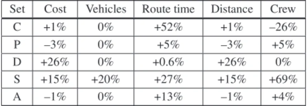
cost, the fleet size employed, the distance travelled by the vehicles, the total crew size (excluding the security guard, and equal to 2 per vehicle), and if the solution is feasible according to the model constraints. For the CPLEX’s solutions, Table 2 presents the number of clusters defined according to the requirements discussed in the beginning of Section 5, the solution cost, the fleet size employed, the distance travelled by the vehicles, the total crew size (variable and equal to the sum of the largest delivery crews in the two possible trips of each vehicle), the number of unserved clusters, and the solutions gap between the best feasible MIP solution found and the LP relaxation. Table 3 summarizes the comparisons by depicting the average percent difference between GAMS/CPLEX’s solutions and the company’s estimated solutions.
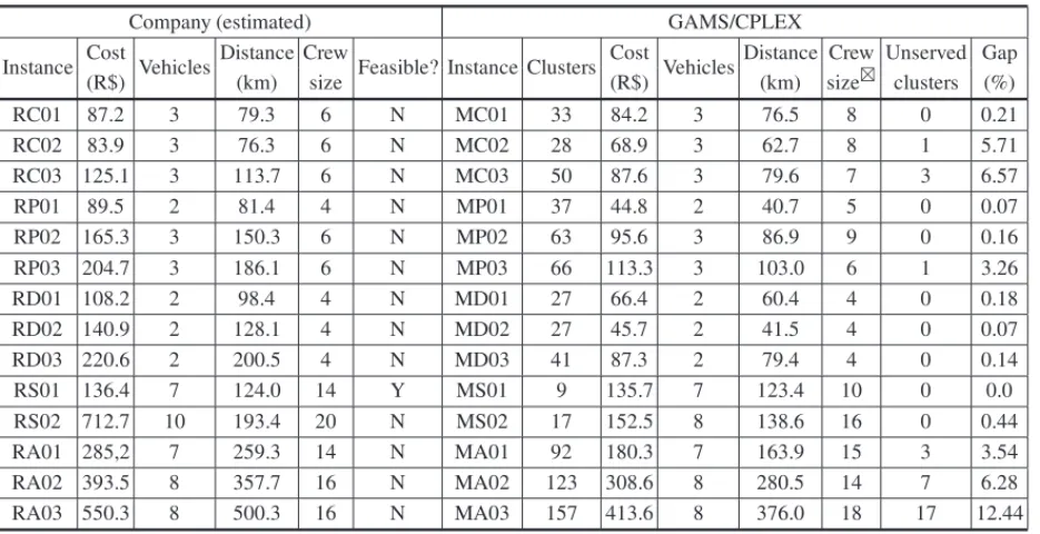
As shown in the sixth column of Table 2, the company’s solutions are infeasible for all instances but one, either for violating route time, time windows, truck capacity or minimum load in the second trip. Even though route scheduling had to be estimated, the company’s logistics operators confirm that such violations are, in fact, very common. As an example, the company’s estimated solution for instance RC02 exhibits violation of the time window upper limit of 3 clusters of restaurants, ranging from 47 to 110 minutes beyond the maximum limit of 120. We note that if we increase the time window upper limit of the only unserved cluster in the corresponding instance MC02 from 120 to 180 minutes (i.e., a 60 minute violation), CPLEX succesfully incorporates the cluster in a route, resulting in a less infeasible option than the company’s solution in less than 100 seconds of computing time.
Table 3 shows that CPLEX produced average reductions in cost, number of vehicles, route time, and travelled distance of 41%, 2%, 30%, 31%, respectively. The improvements were achieved at the expense of only 6% average increase in the number of deliverymen. We note that the large crew size increments in sets C and P compensate the overtime hours present in the company’s solutions (set P) or the clusters’ time windows violation (set C). In fact, overtime accounts for an average of 2:45 h per vehicle in set P and time windows violations accounts for an average of 18 min per cluster with time window in set C. Similarly, the large decrement in set S crew size indicates that some of the vehicles in the company’s solutions are overmanned. This can be clearly observed in the results of instances RS01 (the only case with a feasible company’s estimated route plan) and MS01. Both solutions have equal or very similar costs, number of ve-hicles and total distance, whereas the number of deliverymen is four men larger in the company’s solution. That is, setting the crew size based on the specificities of each trip can indeed bring benefits, either by impeding overtime/time windows violations or overmanning.
JOS
´E
F
E
RRE
IRA
D
E
S
O
U
Z
A
NE
T
O
a
n
d
V
IT
´O
R
IA
P
URE
Z
A
Table 2– Company’s estimated solutions and solutions of model (1)-(18) solved with GAMS/CPLEX.
Company (estimated) GAMS/CPLEX
Instance Cost Vehicles Distance Crew Feasible? Instance Clusters Cost VehiclesDistance Crew Unserved Gap (R$) (km) size (R$) (km) size⊠ clusters (%) RC01 87.2 3 79.3 6 N MC01 33 84.2 3 76.5 8 0 0.21 RC02 83.9 3 76.3 6 N MC02 28 68.9 3 62.7 8 1 5.71 RC03 125.1 3 113.7 6 N MC03 50 87.6 3 79.6 7 3 6.57 RP01 89.5 2 81.4 4 N MP01 37 44.8 2 40.7 5 0 0.07 RP02 165.3 3 150.3 6 N MP02 63 95.6 3 86.9 9 0 0.16 RP03 204.7 3 186.1 6 N MP03 66 113.3 3 103.0 6 1 3.26 RD01 108.2 2 98.4 4 N MD01 27 66.4 2 60.4 4 0 0.18 RD02 140.9 2 128.1 4 N MD02 27 45.7 2 41.5 4 0 0.07 RD03 220.6 2 200.5 4 N MD03 41 87.3 2 79.4 4 0 0.14 RS01 136.4 7 124.0 14 Y MS01 9 135.7 7 123.4 10 0 0.0 RS02 712.7 10 193.4 20 N MS02 17 152.5 8 138.6 16 0 0.44 RA01 285,2 7 259.3 14 N MA01 92 180.3 7 163.9 15 3 3.54 RA02 393.5 8 357.7 16 N MA02 123 308.6 8 280.5 14 7 6.28 RA03 550.3 8 500.3 16 N MA03 157 413.6 8 376.0 18 17 12.44
⊠Largest crew in the two possible trips of each vehicle.
a
O
per
ac
ional,
V
ol.
36(
3)
,
Table 3– Average percentage difference between GAMS/ CPLEX’s solutions and the company’s estimated solutions.
Set Cost Vehicles Route time Distance Crew
C –19% 0% –25% –19% +28%
P –45% 0% –37% –45% +25%
D –58% 0% –29% –58% 0%
S –66% –12% –29% –18% –24%
A –27% 0% –30% –27% +2%
we felt necessary to verify the quality of the solutions obtained within the route planning time used in practice (3 minutes per vehicle). Table 4 presents the results.
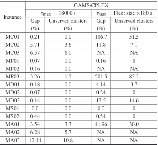
We note in Table 4 that limiting the computation time to the company route planning time results in solutions substantianly inferior, with increases of the travelled distance cost of 58%, 11% and 6% in instances MP01, MD02 and MS02, respectively. For instances MC01, MC02, MP03, MD01, MD03 and MA01, the gaps are substantially higher since the average served clusters goes down to 32%. In other four instances (MC03, MP02, MA02 and MA03) the computational time is not even sufficient to obtain a feasible solution.
Table 4– GAMS/CPLEX performance with two computational times.
Instance
GAMS/CPLEX
τmax=18000 s τmax=Fleet size×180 s Gap Unserved clusters Gap Unserved clusters
(%) (%) (%) (%)
MC01 0.21 0.0 106.7 51.5
MC02 5.71 3.6 11.8 7.1
MC03 6.57 6.0 NA NA
MP01 0.07 0.0 0.16 0
MP02 0.16 0.0 NA NA
MP03 3.26 1.5 501.5 83.3
MD01 0.18 0.0 4.14 3.7
MD02 0.07 0.0 0.24 0
MD03 0.14 0.0 17.5 14.6
MS01 0.0 0.0 0.0 0
MS02 0.44 0.0 0.54 0
MA01 3.54 3.3 41.96 30.0
MA02 6.28 5.7 NA NA
MA03 12.44 10.8 NA NA
We therefore conclude that the time required by CPLEX’s branch-and-cut (and possibly, other exact methods) to generate good quality solutions, makes its use unviable in practical contexts, as one might expect, and points to the investigation of heuristic or hybrid methods. Table 5 presents the results from the application of our GRASP implementation, limited to the route planning time practiced by the company. We also include the number of unserved clusters and the gaps of the solutions found with GAMS/CPLEX for a quick comparison and Table 6 summarizes the differences.
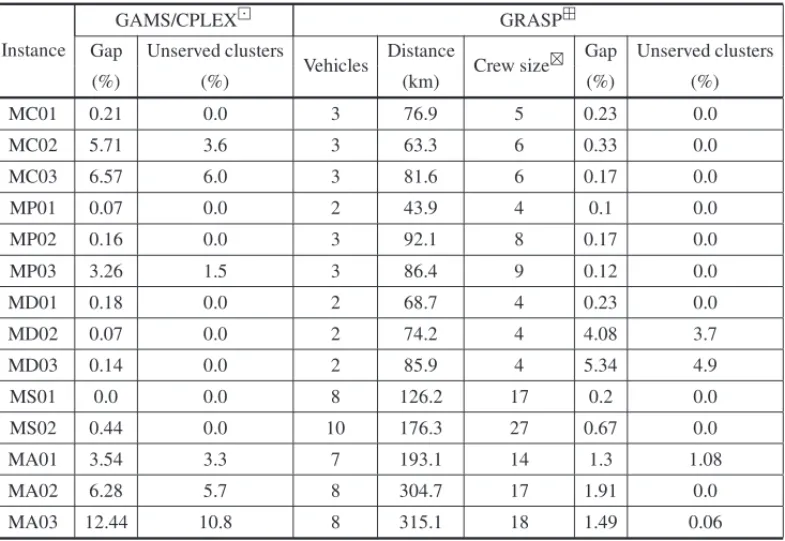
Table 5 shows that GRASP produced solutions with smaller gaps than GAMS/CPLEX in 43% of the instances as the result of a larger number of served clusters. For example, among the 372 clusters of set A, GRASP fails to serve 2 clusters while GAMS/CPLEX’s solutions exhibit 27 unserved clusters. Average gaps with GAMS/CPLEX and GRASP are equal to 2.79% and 1.17%, respectively, indicating that the heuristic approach is capable of generating better quality solutions in much shorter computational times. However, regarding instances MD02 and MD03 (dangerous areas), GRASP’s solutions present an average of 4.3% of unserved clusters. CPLEX’s routes, on the other hand, incorporated all clusters in these two instances.
Table 5– Solutions of model (1)-(18) solved with GRASP.
Instance
GAMS/CPLEX GRASP
Gap Unserved clusters
Vehicles Distance Crew size⊠ Gap Unserved clusters
(%) (%) (km) (%) (%)
MC01 0.21 0.0 3 76.9 5 0.23 0.0
MC02 5.71 3.6 3 63.3 6 0.33 0.0
MC03 6.57 6.0 3 81.6 6 0.17 0.0
MP01 0.07 0.0 2 43.9 4 0.1 0.0
MP02 0.16 0.0 3 92.1 8 0.17 0.0
MP03 3.26 1.5 3 86.4 9 0.12 0.0
MD01 0.18 0.0 2 68.7 4 0.23 0.0
MD02 0.07 0.0 2 74.2 4 4.08 3.7
MD03 0.14 0.0 2 85.9 4 5.34 4.9
MS01 0.0 0.0 8 126.2 17 0.2 0.0
MS02 0.44 0.0 10 176.3 27 0.67 0.0
MA01 3.54 3.3 7 193.1 14 1.3 1.08
MA02 6.28 5.7 8 304.7 17 1.91 0.0
MA03 12.44 10.8 8 315.1 18 1.49 0.06
τmax=18000 seconds.
τmax=Fleet size×180 seconds.
Table 6 – Average percentage difference between GRASP’s solutions and GAMS/CPLEX’s solutions.
Set Cost Vehicles Route time Distance Crew
C +1% 0% +52% +1% –26%
P –3% 0% +5% –3% +5%
D +26% 0% +0.6% +26% 0%
S +15% +20% +27% +15% +69%
A –1% 0% +13% –1% +4%
5.2 A simple hybrid approach
As means to investigate the performance of a hybrid method, we solve the 14 instances with GAMS/CPLEX from the best solution produced by GRASP. Since these best solutions are usu-ally obtained within 40% of the computational time, we set the time for the application of the metaheuristic and GAMS/CPLEX as 0.4 (Fleet size×180) seconds and 0.6 (Fleet size×180), respectively. That is, the time provided to the hybrid method is equal to the route planning time practiced by the company. Table 7 shows the results, along with the number of unserved clus-ters and the gaps of the solutions found by GAMS/CPLEX without the starting solution and
τmax=18000 seconds. Table 8 summarizes the comparisons.
The application of the hybrid method (within the company route planning time) improved 6 of the 14 solutions of GAMS/CPLEX (obtained within 18000 seconds of processing time) regard-ing the number of served clusters. In particular, Table 7 shows that service is provided to all clusters of instances MC02, MC03, MP03 and MA02, despite the fact that the travelled distance is 6.5% shorter. When compared to the solutions provided by GRASP, the average percentage of unserved clusters in instances MD02, MD03, MA01 and MA03 decreases from 2.4% to 0.9%, while solutions for set D exhibit an increased number of served clusters in 2 instances and reduc-tions of 16.5% on the travelled distance. For set S, the improvements are even larger, disclosing an average of 22.2% decrease on the number of vehicles employed. In addition, reductions of 1, 7 and 12 deliverymen are observed in the solutions of instances MP02, MS01 and MS02, respectively, representing a 38.4% savings on the crew size prescribed by GRASP.
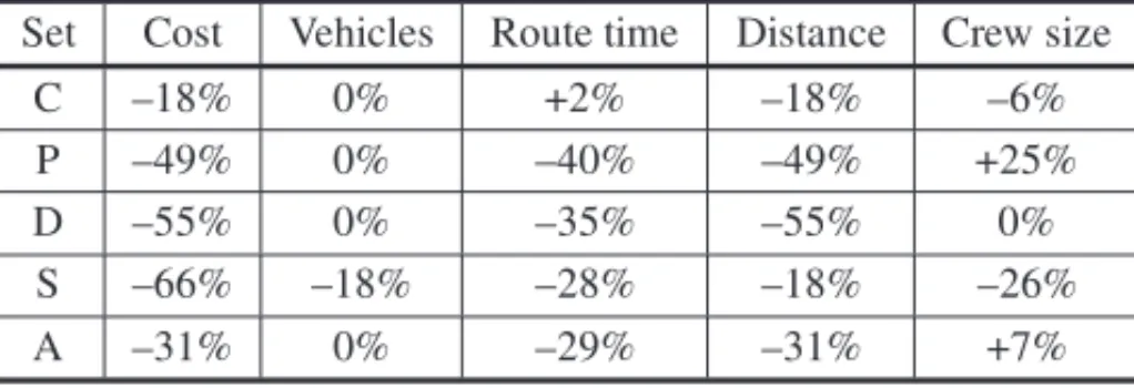
We conclude that the performance of the hybrid method is superior to the other proposed meth-ods, as it combines mostly high quality solutions to low computational time. The method can be considered satisfactory for all instances but MD03, MA01 and MA03; in these cases, an average of 1.2% of the clusters remained unserved (note in Table 2 that all clusters in instance MD03 can actually be served). Table 9 summarizes the comparisons between the hybrid method solutions and the company’s solution.
6 CONCLUSIONS AND PERSPECTIVES OF FUTURE RESEARCH
Table 7– Solutions of model (1)-(18) solved with the hybrid method.
Instance
GAMS/CPLEX Hybrid
Gap Unserved clusters
Vehicles Distance Crew size⊠ Gap Unserved clusters
(%) (%) (km) (%) (%)
MC01 0.21 0.0 3 76.7 5 0.22 0.0
MC02 5.71 3.6 3 63.3 6 0.33 0.0
MC03 6.57 6.0 3 80.2 6 0.16 0.0
MP01 0.07 0.0 2 43.9 4 0.1 0.0
MP02 0.16 0.0 3 85.1 7 0.15 0.0
MP03 3.26 1.5 3 85.9 9 0.11 0.0
MD01 0.18 0.0 2 68.7 4 0.23 0.0
MD02 0.07 0.0 2 44.5 4 0.12 0.0
MD03 0.14 0.0 2 77.8 4 2.65 2.4
MS01 0,00 0.0 7 123.4 10 0 0.0
MS02 0.44 0.0 7 136.2 15 0.43 0.0
MA01 3.54 3.3 7 178.1 14 1.28 1.08
MA02 6.28 5.7 8 285.4 17 1.89 0.0
MA03 12.44 10.8 8 303.7 18 1.48 0.06
τmax=18000 seconds.
τmax=0.4×Fleet size×180 (starting solution produced by GRASP) + 0.6×Fleet
size×180 (improvement produced by GAMS/CPLEX) seconds.
⊠Largest crew in the two possible trips of each vehicle.
Table 8 – Average percentage difference between the hybrid method’s solutions and GAMS/CPLEX’s solutions.
Set Cost Vehicles Route time Distance Crew size
C +1% 0% +35% +1% –26%
P –7% 0% –5% –7% 0%
D +5% 0% –8% +5% 0%
S –1% –7% +15% –1% –4%
A –7% 0% +2% –7% +4%
Table 9 – Average percentage difference between the hybrid method’s solutions and the company’s estimated solutions.
Set Cost Vehicles Route time Distance Crew size
C –18% 0% +2% –18% –6%
P –49% 0% –40% –49% +25%
D –55% 0% –35% –55% 0%
S –66% –18% –28% –18% –26%
A –31% 0% –29% –31% +7%
Sets of instances based on real data provided by the company and comprising 1 to 3 market areas were solved with the branch-and-cut algorithm of the software GAMS/CPLEX, a GRASP meta-heuristic and a simple hybrid method that applies GAMS/CPLEX from the incumbent solution provided by the metaheuristic. In particular, the hybrid method was capable to generate high quality solutions for most of the instances within the route planning time required by the pany, in these cases presenting an impressive average cost reduction of 37% relative to the com-pany’s estimated solutions. It should be emphasized that the resulting solutions were analyzed and validated by the company’s logistic operators, indicating the potential of the application of operations research techniques in real environments. The cases for which the methods failed to route all demand clusters motivate the development of more sophisticated metaheuristics or hybrid methods.
Since limited experiments during this research revealed a close relation between cluster forma-tion and the routing quality, another interesting avenue of research is to study the problem that combines clustering to the routing/scheduling/crew size decisions. Finally, considering uncer-tainties in travel times and/or demand with the application of robust optimization techniques also follows as a suggestion of future research. For instance, it is clear that urban centers are partic-ularly susceptible to traffic jams, which may not justify the trucks travelling times based on an average speed adopted in the present study.
ACKNOWLEDGMENTS
The authors thank the two anonymous reviewers for their useful comments and suggestions, the Brazilian drinks company for its extensive collaboration with this study, and CNPq (grant 304803/2013-8) and FAPESP for their financial support.
REFERENCES
[1] ALONSOF, ALVAREZMJ & BEASLEYJE. 2007. A tabu search algorithm for the periodic vehicle routing problem with multiple vehicle trips and accessibility restrictions.Journal of the Operational Research Society,59: 963–976.
[3] ASSADAA. 1988. Modeling and Implementation Issues in Vehicle Routing.In Vehicle Routing: Methods and Studies, B.L. Golden and A.A. Assad (eds.) North-Holland, Amsterdam, pp. 7–46. [4] AZIN, GENDREAUM & POTVIN J-Y. 2010. An exact algorithm for a vehicle routing problem
with time windows and multiple use of vehicles.European Journal of Operational Research,202: 756–763.
[5] BALDACCIR, TOTHP & VIGOP. 2010. Exact algorithms for routing problems under vehicle capac-ity constraints.Annals of Operation Research,175: 213–245.
[6] BELFIOREP & YOSHIZAKIHTY. 2013. Heuristic methods for the fleet size and mix vehicle routing problem with time windows and split deliveries.Computers & Industrial Engineering,63: 589–601. [7] BODIN L, GOLDENB, ASSADA & BALL M. 1983. Special Issue – Routing and scheduling of
vehicles and crews – the state of the art.Computers & Operations Research,10.
[8] BRAEKERSK, RAMAEKERSK & NIEUWENHUYSEIV. 2015. The vehicle routing problem: State of the art classification and review.Computers & Industrial Engineering.
[9] BRANDAO˜ J & MERCER A. 1997. A tabu search algorithm for the multi-trip vehicle routing and scheduling problem.European Journal of Operational Research,100: 180–191.
[10] BRAYSY¨ O & GENDREAU M. 2005a. Vehicle routing problem with time windows, part I: Route construction and local search algorithms.Transportation Science,39(1): 104–118.
[11] BRAYSY¨ O & GENDREAUM. 2005b. Vehicle routing problem with time windows, part II: Meta-heuristics.Transportation Science,39: 119–139.
[12] BREEDAMAV. 2001. Comparing Descent Heuristic and Metaheuristics for the Vehicle Routing Prob-lem.Computer & Operations Research,28(4): 289–315.
[13] CLARKEG & WRIGHT WJ. 1964. Scheduling of Vehicle from a Central Depot to a Number of Delivery Points.Operations Research,12: 568–581.
[14] CUNHACB. 2000. Aspectos Pr´aticos da Aplicac¸˜ao de Modelos de Roteirizac¸˜ao de Ve´ıculos a Pro-blemas Reais.Transportes, Rio de Janeiro,8(2): 51–74.
[15] DESROISIERSJ, DUMASY, SOLOMONMWP & SOUMISF. 1995. Time constrained routing and scheduling. In: Network Routing, Handbooks in Operations Research and Management Science [edited by Ball MT, Magnanti L, Monma CL & Nemhauser GL.], North-Holland, Amsterdam, pp. 35– 139.
[16] FEOTA & RESENDEMGC. 1995. Greedy Randomized Adaptive Search Procedures.Journal of Global Optimization,6: 109–134.
[17] FERREIRAVO & PUREZAV. 2012. Some experiments with a savings heuristic and a tabu search approach for the vehicle routing problem with multiple deliverymen.Pesquisa Operacional,32: 443– 463.
[18] FLEISCHMANNB. 1990. The vehicle routing problem with multiple use of vehicles. Working paper. Fachbereich Wirtschaftswissenschaften, Universit¨at Hamburg.
[19] GRANCYGS & REIMANNM. 2014a. Vehicle routing problems with time windows and multiple service workers: a systematic comparison between ACO and GRASP.Central European Journal of Operations Research.
[21] MUNARIP & MORABITOR. The vehicle routing problem with time windows and multiple deliv-erymen: exact solution approaches. S˜ao Carlos – SP: [s.n.]. Available in:< http://www.optimization-online.org/DB HTML/2016/01/5289.html>.
[22] OLIVERA A & VIERA O. 2007. Adaptive memory programming for the vehicle routing problem with multiple trips.Computers and Operations Research,34: 28–47.
[23] OSMANIH. 1993. Metastrategy simulated annealing and tabu search algorithms for the vehicle rout-ing problem.Annals of Operation Research,41: 421–452.
[24] PARRAGHS, DOERNERK & HARTLR. 2008. A survey on pickup and delivery problems.Journal f¨ur Betriebswirtschaft,58: 21–51.
[25] PETCHRJ & SALHIS. 2004. A multi-phase constructive heuristic for the vehicle routing problems with multiple trips.Discrete Applied Mathematics,133: 69–92.
[26] PUREZAV, MORABITOR & REIMANNM. 2012. Vehicle routing with multiple deliverymen: Mod-eling and heuristic approaches for the VRPTW.European Journal of Operational Research,218: 636–647.
[27] RONEND. 1988. Perspectives on pratical aspects of truck routing and scheduling.European Journal of Operational Research,35(2): 137–145.
[28] SALHIS & PETCHRJ. 2007. A GA based heuristic for the vehicle routing problem with multiple trips.Journal of Mathematical Modelling and Algorithms,6: 591–613.
[29] SCHNEIDERM, STENGERA & GOEKED. 2014. The Electric Vehicle-Routing Problem with Time Windows and Recharging Stations.Logistics Planning and Information Systems,48(4): 500–520. [30] SEIXASMP & MENDESAB. 2013. Column generation for a multitrip vehicle routing problem with
time windows, driver work hours, and heterogeneous fleet.Mathematical Problems in Engineering, http://dx.doi.org/10.1155/2013/824961.