ABSTRACT: This study presents an empirical examination of climate change related to vulnerabil-ity impacts on food securvulnerabil-ity and remedial adaptation options as a suitable strategy by prioritizing needs over a 50-year period. An Empirical Dynamic Commutable General Equilibrium Model for Climate and the Economy (EDCGECE) is applied using future strategies for Malaysia against a baseline scenario of existing conditions, following the top-down options. The model takes into account various climatic variables, including climatic damage, carbon cycle, temperature and rainfall fluctuation, carbon emissions, vulnerability and carbon concentrations, which were adapted from national observational predictions of climatic changes caused by global warming from 2015 to 2065. The results prioritize climate change mitigation for the future. Specifically, this study estimates Malaysia’s food sustainability prospects without adaptation actions and with 5 % to 20 % adaptation actions overtime in different adaptation scenarios, as contrasted with the baseline. The results indicate that food sustainability cost in the baseline in 2015 is 859.3 million US Dollar (USD), which is about a 30-35 % shortage compared with the national targets, and that the shortage will rise over time to USD 987.3 million in 2065. However, the cost of applying different levels of adaptation for food sustainability over time is rising considerably. However, the residual damage also decreases with all adaptation actions in the different scenarios. Thus, adaptation shows a positive sign for Malaysia’s agricultural sectors. As growth values are posi-tive and show rising trends, therefore the projected adaptation policy can be effecposi-tive for food sustainability for sustainable future strategies in Malaysia.
Keywords:CGE,policy development, strategies, agricultural sustainability 1University of Malaya/IGS, 50603 Kuala Lumpur − Malaysia.
2Universiti Teknologi Malaysia/IBS, 54100 Kuala Lumpur − Malaysia.
3University of Malaya/Faculty of Science − Dept. of Science & Technology Studies.
4University of Malaya/FEA − Dept. of Economics. *Corresponding author <[email protected]>
Edited by: Carlos Eduardo Pellegrino Cerri
Agriculture and food security challenge of climate change: a dynamic analysis for
Ferdous Ahmed1*, Abul Quasem Al-Amin2, Zeeda Fatimah Mohamad3, Santha Chenayah4
Received April 07, 2015
Accepted October 19, 2015
Introduction
Climate change is currently one of the most chal-lenging threats that the world faces. The scientific evi-dence is overwhelming and climate change is recognized as a serious problem that demands an urgent response (Al-Amin and Filho, 2014). It is now established that climate change has overwhelmed traditional climatic patterns, severely affecting most developing nations (Chambwera and Stage, 2010; Pachauri et al., 2014; Nelson et al., 2014; Fankhauser, 2013; Kurukulasuriya and Rosenthal, 2013; Wheeler and Braun, 2013; Hansen et al., 2013; Porter et al., 2014; Downing, 2013; Nelson et al., 2010; Holzworth et al., 2015; Furman et al., 2014; Williamson et al., 2014; Adger et al., 2013; Calzadilla et al., 2013). As the back-ground to research on climate change, there is, of course, a number of recognized studies in the literature on the mat-ter, including Lobell et al. (2011), Rowhani et al. (2011), Georgescu et al. (2011), Ahmed et al. (2011), Burke et al. (2010), Hertel et al. (2010), Bonfils et al. (2008), Lobell and Field (2007), Cahill et al. (2007) and Parry (2007). Al-though there was a positive agreement among developed countries at the 20th COP Convention in Lima, Peru 2014,
to decrease carbon emissions to within a certain level, this will take time and it will be necessary to wait and see the reality for the future (COP-20, 2014).
Al-Amin et al. (2015) reported that the damage to food production in Malaysia might be up to 4-6 % per 1
°C temperature variation due to climate change and
tra-ditional climatic patterns. Not only will the food security issue be exacerbated for climate change, but the whole economy of a state may also be at stake, and the Ma-laysian economy will be no exception. Moreover, there is still a food security gap in the Malaysian economy, which is assessed at about 30-35 % from the current demand. Thus, climate change could worsen the food security gap from the current level at year 2014 over time. Therefore, the fundamental question relies on how Malaysia can achieve self-sufficiency for food security, given the rising demands on agriculture and foodstuffs, by managing the climatic issues. Thus, we propose a rel-evant explanation of the fundamental question from the Malaysian perspective and introduce some new ideas and concepts regarding the challenges to policy guide-lines to achieve long-term expositions of possible devel-opments. Therefore, an adaptation option is considered for the scientific establishment on agriculture and food-stuffs (Figure 1). The findings of our study may be useful for Malaysian policy-makers dealing with the impacts of climate change. Finally, this study aims to achieve a cer-tain food security option with positive impacts on the Malaysian economy.
Materials and Methods
This study uses economic, earth sciences and eco-logical approaches to climate change in weighing options dealing with an applicable assessment aimed at reducing
climatic impacts for the long term. To identify and priori-tize the needs for climate change adaptation, the Empiri-cal Dynamic Commutable General Equilibrium Model for Climate and the Economy (EDCGECE) is considered in this study. Mainly, it uses an economic inquiry to con-vert all economic activities and impacts into a common unit for the total amount and then it calibrates in the com-mon unit based on current economic data generated by the Malaysian Social Accounting Matrix (SAM). The mod-el links climatic factors such as climatic damage, carbon cycle, temperature and rainfall fluctuation, carbon emis-sions, vulnerability and carbon concentration that affect economic growth, and it takes certain variables such as national population, the national targeted aim and agen-das for food sustainability, as assumed or specified. Other related variables of the SAM are generated by the model and are endogenous in nature. These endogenous vari-ables include capital stock, output, temperature change, and climatic damage. In contrast, the exogenous variable is the corrective adaptation policy thrust, applying differ-ent levels of adaptation to food sustainability over time. The measurable units are the value of goods and services (including vulnerabilities) in 2015 and current Malaysian prices. Mainly, the EDCGECE integrated model sees the concept of economic theory such as national growth, capi-tal investment, consumption, interest rates, and national thrust, and thereby it considers today’s growth along with all the related climatic effects and vulnerabilities to sus-tain future growth. The details of our study materials and approaches are given below.
Climate change in the EDCGECE
The impacts of climate change are entered into our study model as monetized damage, and aggregate
mon-etized gross damage (namely GD) is modeled as a func-tion of the climate variable. Thus, the gross damage as a function of the climate variable is given as:
GDt =αi∆Tt
2 (1)
The climate change that affects the economy is considered to be quadratic (or at least the power is great-er than 1) and this allows the climate impact function to be a function of climatic factors:
Tt = ajTt–1 + akEMt (2)
Here, exogenous shocks assumed as an increase in emissions (EMt) by a certain amount lead to an increase in the climate impact function (Tt) compared to the level of the preceding period. The damage grows linearly with output Qx, which is a constant fraction of the national output of commodities (denoted as c in the standard ap-plied general equilibrium modelling equations). This lin-ear trend may be influenced by further factors that shift the amount of damage up and result in a change of the affecting valuation:
Emt = Ω . Qxt (1 – mt –ALt) (3)
The cost of adaptation depends on the output as well as the adaptation level, while the gross damage de-pends on the output and emission values as follows:
AC
Qx AL
t t
t t
=γ1− ⋅ γ2 (4)
GD
Qx M
t t
t
=ω⋅ (5)
The gross damage (GD) of climate change is ex-pressed as a function of the climate variables:
GD
Qx T T
t t
t t
=α∆ +α∆ α
1 2
3 (6)
To obtain the monetary value of gross damage (GD) as a percentage of output (Qx), it is considered as a summation of RDt(residual damage) and ACt (adaptation costs):
GD Qx
RD GD AL AB Qx
AC AL AB Qx
t t
t t t t t
t t t t
=
(
, ,)
+(
,)
(7)Gross damage as a percentage of output depends on the residual damage and the adaptation cost for a certain adaptation level. Thus, the value of the residual damage depends on the gross damage GDtand adapta-tion level ALt.
Study area
The climate measurements used in this study were carried out in the East and West of Malaysia. All the national climatic data come from the four towns of Kuching (Sarawak) and Kota Kinabalu (Sabah) in eastern Figure 1 − Getting started leads to study the gap identification for
Malaysia, and Kuantan (Pahang) and Petaling Jaya (Se-langor) in western Malaysia, located at 1°25'0" N and 110°20'0" E, 5°58'50" N and 116°4'37" E, 3°48'0" N and 103°20'0" E and 3°5'0" N and 101°39'0" E, respectively.
Empirical economizing
The scenario and assessment involved in this study use the EDCGECE with the adoption of empirical econo-mizing to observe the complex interaction between glob-al warming and climate variability, with capitglob-al stock, carbon concentrations, carbon emissions, temperature and rainfall fluctuations, and agricultural productivity. The economizing measurements mean a range of reason-able climatic outcomes from the years 2015 to 2065 and are endogenous in nature. The adopted modelling takes a top-down approach, focusing on the impacts on Malay-sia given a wide range of likely climate outcomes related to a specific climate prediction on a global level adjusted to country-specific level. The EDCGECE is constructed by applying national observational large-scale data to: (a) the predicted annual cycle of observed regional tem-perature and rainfall, and (b) the predicted annual cycle observed in large-scale circulation fields (western and eastern Malaysia).
The EDCGECE subsequently included the yearly average circulation parameters as predictor variables and the yearly average temperatures and rainfall fluc-tuations with carbon concentrations as predicted vari-ables to determine changes in large-scale exchange over time. All large-scale predictor data used in this study was taken from the climate change scenarios for Malay-sia 2001-2090 projected by the MalayMalay-sian Meteorologi-cal Department (MMD, 2009). The national temperature variations, derived from historical records, were applied to the EDCGECE to project changes in large-scale varia-tions by the concentravaria-tions of Green House Gases (280 parts per million - ppm - in pre-industrial times to 650 ppm in 2065). This study considers the quantitative analysis. Figure 2 shows the steps and procedures for this study and how MCE (Malaysian Climatic Equations) were embedded into the EDCGECE. However, some modifications were made to the data obtained from the SAM and MMD to fulfill the study scope. The annual cycle of local temperatures adopted for the EDCGECE is based on locations at 1°25'0" N and 110°20'0" E, 5°58'50" N and 116°4'37" E, 3°48'0" N and 103°20'0" E and 3°5'0" N and 101°39'0" E to capture the long-term temperature effects with a standard elevation set-up for the years 2015 to 2065.
Two datasets are used in this study. The first one is from macroeconomic variables such as data from the Malaysian national accounts (DOS, 2010, 2013a, b; MDP, 2010). This study modified the SAM as construc-tion of the SAM from different data sources for different periods. Subsequently, the SAM was updated and bal-anced by a cross-entropy process. The second dataset is from the Meteorological Department on climate change and meteorological parameters (MMD, 2009; NAHRIM,
2006). The data on climate change, particularly meteoro-logical (i.e. climatic) parameters, were used for the sce-nario exercise based on two monsoons and four seasons from 1969 to 2007 to apply the baseline year in 2015. The summer monsoon data are categorized as the south-west monsoon (SM), which influences the climate of Ma-laysia from May to September. The winter monsoon is categorized as the northeast monsoon (NM), which influ-ences the climate from November to February (Al-Amin and Leal, 2014). The modeling adopted in the EDCGECE helps to quantify the likelihood of exceeding thresholds as core data for impact and vulnerability until the year 2065. The threshold variable data are: (a) the probabil-ity of unforeseen climatic shocks in present and like-ly future (i.e. 2065) climate situations, and (b) climate vulnerabilities with their likely impacts. This study has selected several diverse scenario data of temperatures between 0.8 and 3.1 °C and 280-650 ppm carbon con-centration (CO2) with certain levels of fluctuation with several climatic damage intercepts.
Study of the different levels of adaptation options for climate change
This study has also used the extensions of AD-DICE and AD-RICE modelling. To compare the different levels of adaptation options, we followed the AD-RICE model (de Bruin et al., 2009), which defines the opti-mum level of adaptation using the following equation:
ALt w M
t
=
− .
. γ γ
γ
2 1 1 21
where (
ω
j.Mt) is the equivalent value of the gross dam-age (GD) that we found from the Malaysian model, and the rest of the parameters are adaptation coefficients de-Figure 2 − Process of Empirical Dynamic Commutable Generalfined in Equation (4). We estimated the value of these coefficients from the AD-RICE model adapted for a income country (Malaysia is currently a middle-income country). We also considered the values of these coefficients exogenously from the AD-RICE model to our EDCGECE to achieve the optimum level of adaptation and support sustainable future strategies (Figure 3).
Description of simulations
In this study, we estimated the impacts of climate change over a 50-year period. We divided the 50 years into five 10-year different segments, which are indepen-dent of each other. We considered 2015 as the bench-mark year (base year) for this study to simulate the sce-nario outcomes. Therefore, all the simulations start from this benchmark year and end in 2065. Table 1 shows time segments 1 to 5, starting in year 2015 and ending in year 2065.
Results
This study seeks to focus on different damage lev-els, such as gross damage, residual damage and net dam-age. All these categories of damage are discussed based on different scenarios with reference to different adap-tation actions, and these calibrated adapadap-tation scenarios are finally compared with the baseline. In the case of re-sidual damage, this is presented with adaptation actions
(Figure 3), as residual damage scenarios with different adaptation actions, net residual damage (Figure 4) and comparing different scenarios with the baseline. In par-ticular, the impacts of taking no adaptation actions are shown in Figure 3. Obviously, as seen in Figure 3, if no adaptation action takes place then the residual damage according to our optimized model will increase gradu-ally. Thus, the residual damage is RM 1746.86 million in baseline 2015, but in 2065 it shows a rapid increase up to RM 2017.94 million without any adaptation actions. The findings show an increase in trends of damage in all segments of the study period, namely from 2015 to 2025, from 2025 to 2035, from 2035 to 2045, from 2045 to 2055 and from 2055 to 2065.
However, this study also focuses on different sce-narios of residual damage, applying different levels of adaptation ranging from 5 to 20 %. Figure 3 shows the different scenarios of residual damage. Specifically, it shows that the residual damage is decreased significant-ly with reference to the baseline after implementing 5 % adaptation policies. The trend of residual damage for other scenarios taking 10, 15 and 20 % adaptation poli-cies is similar, as it gradually declines compared with the baseline values of each segments of 2015. Thus, the findings justify the rationale for the adaptation actions in different scenarios from 2015 to 2065. On the other hand, comparing all the scenarios of net residual damage with the baseline, we find that all the values are negative in Figure 4. These findings provide further clarification of our forecasts and scenarios. Thus, by taking adapta-tion opadapta-tions, these projecadapta-tions show the emergence of positive signs in the Malaysian agricultural sector.
Results, thus, show that the adaptation policy for Malaysia is positive in reducing the effect of climate change on food sustainability and future issues regard-ing food security. Importantly, the cost of applyregard-ing the 5 % adaptation policy will be below RM 1 million based on the baseline 2015 until 2065. The comparative find-ings are shown in Figure 5, with the rationale for why
Figure 3 − Residual damage with and without adaptation action in different scenarios (million Malaysian Ringgit).
Figure 4 − Net residual damage in different scenarios with baseline (absolute value in million Malaysian Ringgit).
Table 1 − Time segments for the scenario studies.
Time segment 1 Year 2015
Time segment 2 Year 2025
Time segment 3 Year 2035
Time segment 4 Year 2045
Time segment 5 Year 2055
the cost of adaptation would be higher over time. It is important to know the causes, as the adaptation cost will rise progressively if a higher percentage of adaptation pol-icy is applied. The cause is apparent, as the higher level of adaptation trends needs to increase over time to ensure food sustainability and that a higher level of adaptation is required because the continued economic activities also cause climate change and gross damage over time. For example, if the 10 % adaptation policy is applied based on the baseline (2015), then the cost will be about USD 3.6 million. If the 15 % adaptation policy is applied based on the baseline (2015), then the cost will be about RM 53 mil-lion and just over USD 14.4 milmil-lion in 2065. If the 20 % adaptation policy is applied based on the baseline (2015), then the cost will be about USD 40.2 million in 2015 and RM USD 46.5 million in 2065 (Figure 5).
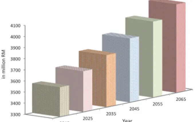
This study considers several adaptation costs in ag-riculture as government expenditure and as a percentage of the Gross Domestic Product (GDP) and it compares their comparative dimensions based on impacts on other related macroeconomic variables. The likely figures of our findings over time are shown in Figures 6 and 7. Many studies consider a level of adaptation of about 10 % as optimal. As we find that an adaptation level greater than 10 % gives higher benefits, we tried to increase it based on the country’s specific conditions and related to other agricultural issues such as food sustainability and food security over time in Malaysia. Figures 6 and 7 show the estimated values of government expenditure before and after the adaptation policy, respectively. Our findings show that the general trend with continued eco-nomic activities shows a linear increase in government expenditure over time after applying different adapta-tion scenarios, as shown in Figure 7.
Government expenditure is essential for the imple-mentation of public policies. Thus, to enforce adaptive
actions, the government has to bear the adaptation costs. The costs in terms of percentages of GDP and govern-ment expenditure must be identified and it is important to find and allocate the resources to different adaptation level options for food security. In particular, this study evaluated the different adaptation costs in terms of per-centages of GDP and government expenditure with and without adaptation to contrast the results of the differ-ent scenarios. Clearly, governmdiffer-ent expenditure would be higher with adaptation than without adaptation costs, but the additional costs of adaptation here are found to be marginal compared to the damage in terms of mon-etary value and percentage change (Figure 7). These findings can be seen from the scenario outcomes with and without adaptation actions in Figures 6 and 7. Find-ings relating to the different levels of adaptation actions show that even for the year 2065, the additional adapta-tion costs of supporting sustainable future strategies are marginal.
According to our main objective, food sustainabil-ity over time has been prioritized to investigate the long-term scenarios of food security and food sustainability for Malaysia. Figure 8 shows the different outcomes for food sustainability over time with and without adapta-tion acadapta-tions with reference to the baseline and with
ad-Figure 5 – Comparison of adaptation costs in different levels with baseline in different scenarios (million Malaysian Ringgit).
Figure 6 − Government expenditure without adaptation actions (million Malaysian Ringgit).
justment actions over time in different adaptation sce-narios, and finally, the various differentiated scenarios compared with the baseline over time. The findings indicate that after applying different adaptation levels over time, food sustainability rose considerably (Figure 9). Specifically, in Figure 8, the findings project that food sustainability in the baseline year 2015 will cost USD 859.3 million and USD 987.3 million in 2065, without adaptation actions, but comparatively it shows a prog-ress of 10 % or more in different adaptation scenarios.
Thus, food sustainability in the baseline year 2015 costs USD 861.9 million with a 10 % adaptation level, USD 872.1 million with a 15 % adaptation level, and higher adaptation levels show higher progress over time. Similarly, food sustainability in 2065 will cost USD 990.2 million at a 10 % adaptation level, USD 1,002.1 million at a 15 % adaptation level, and higher adaptation lev-els also show higher progress. The scenarios contrasted with the baseline and over time are found to be progres-sive and food sustainability rises proportionately as the percentage of adaptation policy is considered higher. As the growth values are positive and show a rising trend in
this study, the clearly projected adaptation actions can, thus, be considered an applicable policy option for food sustainability in Malaysia.
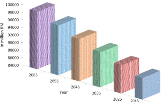
Further, Figures 10 and 11 are related to Real Gross Domestic Product (RGDP) as, considering poli-cies, the outcomes related to RGDP and adaptation op-tions are important to find. Thus, Figure 10 shows the Real Gross Domestic Product (RGDP) without any ad-aptation policy and Figure 11 indicates different RGDP scenarios after taking into consideration different adap-tation actions over time (from 2015 to 2065). We have considered the estimation of Real Gross Domestic Prod-uct (RGDP) because it is a vital issue for Malaysia to justify and understand the importance of the adaptive actions to be considered from an economic viewpoint. According to our findings, the RGDP figures as projected progress are in line with the different levels of adapta-tion acadapta-tions. Adaptaadapta-tion acadapta-tions between 5-15 % reflect a rising RGDP, but applying a 20 % adaptation action results in an abrupt decline in RGDP. This shows that the 20 % adaptation action level is not appropriate to the current national agenda to ensure food security. Some
Figure 8 − Food sustainability over time without adaptation actions (million Malaysian Ringgit).
Figure 9 − Food sustainability over time with different adaptation actions (million Malaysian Ringgit).
Figure 10 – Real Gross Domestic Product (RGDP) without an adaptation policy (million Malaysian Ringgit).
critical factors need to be considered before applying that level of adaptation action to overcome the decline in RGDP.
Figure 10 and 11 indicate the benefits of RGDP in different adaptation scenarios from different actions in terms of their comparative dimensions. The figures indicate policy actions that are suitable and appropriate to consider further as concerns the food sustainability issue. According to the projections, we find that, without adaptation actions, the RGDP in 2015 would be USD 111,998.3million, USD 115,2923 million in 2025, USD 118,677.1 million in 2035, USD 122,149 million in 2045, USD 125,717.4 million in 2055, and USD 129,378.74 million in 2065. Conversely, with a 5 % adaptation ac-tion, the RGDP increases from the baseline in 2015 to USD 17.8 million, to USD 18.3 million in 2025, to USD 17.2 million in 2035, to USD 19.6 million 2045, to USD 18.47 million in 2055, and to USD 20.8 million in 2065. The trend is progressive over time with a higher level of adaptation action, except for 20 %. We performed a cost-benefit analysis of the trends related to the issue of climate change and challenges for food security and support for sustainable future strategies. The economic theory suggests that for any kind of policy action where the benefit is higher than the cost, then, obviously that policy option is suitable to be considered.
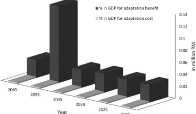
Thus, according to our findings, the percentage in GDP for the adaptation cost (USD) in 2015 is 0.00055 and the benefit is 0.00725, the percentage in GDP for adaptation in 2025 is 0.00055 and the benefit is 0.00728, the percentage in GDP for adaptation in 2035 is 0.00055 and the benefit is 0.00781, the percentage in GDP for adaptation in 2045 is 0.00055 and the benefit is 0.0073, the percentage in GDP for adaptation in 2055 is 0.00055 and the benefit is 0.063 and, finally, the percentage in GDP for adaptation in 2065 is 0.00057 and the benefit is 0.00734 (Figure 12). It is evident that the benefits of ad-aptation are higher than the costs for each time segment in terms of both monetary value and percentage change (Figure 12). This implies that the benefit over cost ratio will continue to increase over the period.
Discussion
Regarding references, most impacts of climate change on agricultural and climatic policy are presented as either global or regional. However, the impacts and costs of climate change cannot be optimally determined on a global basis, as they vary with the changing geo-graphical status both within a country and between countries. Therefore, it is necessary to evaluate the vi-ability of the country’s impending selection of an ap-propriate adaptation policy to support sustainable future strategies in order to address the food security challenge. Considering the importance of the agricultural sector for the Malaysian economy, this study evaluates the impact of climate change and tries to find a suitable adaptation option to support future agro-food sustainability strate-gies. The key questions to answer are: which level of adaptation is appropriate for a tropical country like Ma-laysia? What will be the estimated cost of adaptation? How does this adaptation affect the agricultural sector in maintaining Malaysia’s targeted food sustainabil-ity vision? This study shows that, with continued eco-nomic activities that cause climate change, along with increased gross damage values, the optimum level of ad-aptation trends (5-20 %) to maintain food sustainability increase over time.
According to the results and findings of this study, the proper level of adaptation depends on the continu-ing change in temperature, emissions, economic growth, population growth, and it is based on changes in other related climatic variables for each time segment. This study suggests that a different level of adaptation over time is effective in terms of the decrease in climate change and its negative impacts. This study showed an increasing trend in the cost of adaptation over the 50 years from 2015 to 2065. The growing economic activi-ties that are causing climate change and the associated damage reduction options would cause the required level of adaptation to increase over time. This study focused on reactive adaptation actions and studied the benefits and costs of adaptation. In the case of the ag-ricultural sector, reactive adaptation is particularly rel-evant rather than a pro-active response, especially in developing countries, since this sector is a substantial source of national income for developing countries and the adaptation is to be effective within a very short ges-tation period. The findings are similar to related studies particularly those addressed by the Stern reports (Stern, 2007) and United Nations Framework Convention on Climate Change (UNFCCC) estimates.
As a step ahead toward food sustainability, our study considered an Empirical Dynamic Commutable General Equilibrium Model for Climate and the Econo-my (EDCGECE) model in which the impacts of climate change are influenced by relevant climatic change as ad-dressed in the introduction. We also investigated the im-pacts of climate change adaptation policy with its associ-ated costs on agricultural food security. In addition, this Figure 12 – Comparison of adaptation benefits and costs in % of
study evaluated the costs of adaptation in terms of the percentage of GDP, as macroeconomic costs. The results from the simulations showed that the costs of adaptation are a small percentage of the estimated GDP. Interest-ingly, the results showed that the costs of early actions are small, whereas if the adaptation is to be taken in the later periods, the cost will increase as a GDP percentage. Furthermore, the results established that, for the agricul-tural sector, the adaptation cost is very small as a GDP percentage. These estimations are found to be similar to some earlier global estimates. For example, subject to the aggregation criteria, funding adaptation would be indi-cated by 0.1 % of the industrialized regions as a percent-age of the national GDP (Stephan and Schenker, 2012).
Based on the findings of the study, a suitable ad-aptation policy can be suggested for implementation by Malaysian policy-makers. This proposition is valid be-cause our research showed that the impacts of climate change are projected to increase overtime, which will ultimately reduce the outputs of all economic sectors. Hence, it is the government’s responsibility to formu-late the optimum adaptation policy so that the benefits of adaptation could be achieved collectively. Taking into account these facts, our study has taken initiatives to identify the best ways to ensure food security and sus-tainability over time.
We found different optimum levels of adaptation with different climate conditions in different time seg-ments. Our suggestion to policy-makers is to implement this policy with the investment necessary to improve awareness and change attitudes of Malaysians toward adopting the new policy. The issues highlighted in this study are not new in some developed countries, but are quite new for the development and advances of develop-ing countries. Thus, some critical issues need to be con-sidered effectively in developing countries, as there may be some advantages and disadvantages in solving the new research issues addressed in this study. Though there are some complications in estimating the economic impacts of climate change to determine the most favorable adapta-tion policy, due to the allocaadapta-tion of resources for a suitable option, the study has the following strengths: (a) impacts and costs of the climate change measures cannot be opti-mally determined on a global basis as they are different for other countries, but they have been solved here for the case of Malaysia; (b) the impacts of climate change can af-fect each sector of the economy differently. Agriculture is one of the most vulnerable sectors as it depends directly on weather conditions. It is also the most important sec-tor as it is directly related to food security and economic development, which are addressed in this study, and (c) appropriate adaptations can greatly reduce the magnitude of the impacts of climate change. Existing knowledge re-garding the adaptive capability and adaptation options is not sufficient in Malaysia. Therefore, there is the issue regarding lack of reliability in future projections of adap-tation options and policy and the associated costs in terms of monetary value, as highlighted in this research.
The ultimate contribution of this study is a better understanding of the macroeconomic effects of adapta-tion policies on the Malaysian economy. Specifically, the study enhances current knowledge on: (a) setting up a long-term national climate change adaptation policy framework for Malaysia in response to Malaysian na-tional policy on climate change, (b) filling in the research gap by determining the distribution of impacts on adap-tation costs for the agricultural sector, and (c) formulat-ing guidelines for policy-makers in the macroeconomic measurement unit with accurate data on the overall impacts of adaptive measures to support sustainable fu-ture strategies. Although the ultimate target groups are principally Malaysian policy-makers, a wide range of people and organizations are expected to benefit due to the general nature of the scientific outcome of this study. In essence, it is evident that the adaptation benefits are greater than its costs for every time segment analyzed. Furthermore, the adaptation benefits tend to increase at a higher rate than the increase rate of the costs overtime. This implies that the benefits to cost ratio will contin-ue to increase over time. Conseqcontin-uently, the adaptation policy will be effective for Malaysia in terms of the sce-narios for costs and benefits.
Conclusion
This study used simulation-based dynamic model (EDCGECE) to examine the various adaptation actions toward the food sustainability strategies over time in Malaysia.
Specifically, the study identified that without ad-aptation actions, the maximum food sustainability cost is USD 859.3 million in 2015, which is about a 30-35 % shortage and the shortage would be USD 987.3 million in 2065, which is more than a 40 % shortage from the national targets. Thus, a suitable adaptation for the agri-cultural sector is necessary, as justified by our short- to long-term adaptive modelling.
knowledge of the overall impacts of long-term adaptive measures. Thus, the suggested guidelines enhance the current knowledge needed to establish a long-term na-tional adaptation policy.
Acknowledgements
This study is supported by the project fund-ing RG157-12SBS, University Malaya Research Grant (UMRG)-SBS. The authors would like to thank Univer-sity of Malaya for this financial support.
References
Adger, W.N.; Barnett, J.; Brown, K.; Marshall, N.; O'Brien, K. 2013. Cultural dimensions of climate change impacts and adaptation. Nature Climate Change 3: 112-117.
Ahmed, S.A.; Diffenbaugh, N.S.; Hertel, T.W.; Lobell, D.B.; Ramankutty, N.; Rios, A.R.; Rowhani, P. 2011. Climate volatility and poverty vulnerability in Tanzania. Global Environmental Change 21: 46-55.
Al-Amin, A.Q.; Leal Filho, W. 2014. A return to prioritizing needs: adaptation or mitigation alternatives? Progress in Development Studies 14: 359-371.
Al-Amin, A.Q.; Rasiah, R.; Chenayah, S. 2015. Prioritizing climate change mitigation: an assessment using Malaysia to reduce carbon emissions in future. Environmental Science & Policy 50: 24-33.
Bonfils, C.; Duffy, P.B.; Santer, B.D.; Wigley, T.M.; Lobell, D.B.; Phillips, T.J.; Doutriaux, C. 2008. Identification of external influences on temperatures in California. Climatic Change 87: 43-55.
Burke, M.B.; Miguel, E.; Satyanath, S.; Dykema, J.A.; Lobell, D.B. 2010. Climate robustly linked to African civil war. Proceedings of the National Academy of Sciences 107: E185-E185.
Cahill, K.N.; Lobell, D.B.; Field, C.B.; Bonfils, C.; Hayhoe, K. 2007. Modeling climate and climate change impacts on wine grape yields in California. American Journal of Enology and Viticulture 58: 414A-414A.
Calzadilla, A.; Rehdanz, K.; Betts, R.; Falloon, P.; Wiltshire, A.; Tol, R.S. 2013. Climate change impacts on global agriculture. Climatic Change 120: 357-374.
Chambwera, M.; Stage, J. 2010. Climate Change Adaptation in Developing Countries: Issues and Perspectives for Economic Analysis. International Institute for Environment and Development, London, UK.
COP-20. 2014. The cornerstone for commitment to the future of our climate. Available at: http://www.cop20lima.org/ [Accessed Dec. 10, 2014]
Downing, T.E. 2013. Climate Change and World Food Security. Springer Science & Business Media, Berlin, Germany.
Fankhauser, S. 2013. Valuing Climate Change: The Economics of the Greenhouse. Routledge, New York, NY, USA.
Furman, C.; Roncoli, C.; Nelson, D.R.; Hoogenboom, G. 2014. Growing food, growing a movement: climate adaptation and civic agriculture in the southeastern United States. Agriculture and Human Values 31: 69-82.
Georgescu, M.; Lobell, D.B.; Field, C.B. 2011. Direct climate effects of perennial bioenergy crops in the United States. Proceedings of the National Academy of Sciences 108: 4307-4312.
Hansen, M.C.; Potapov, P.V.; Moore, R.; Hancher, M.; Turubanova, S.A.; Tyukavina, A.; Townshend, J.R.G. 2013. High-resolution global maps of 21st-century forest cover change. Science 342: 850-853.
Hertel, T.W.; Burke, M.B.; Lobell, D.B. 2010. The poverty implications of climate-induced crop yield changes by 2030. Global Environmental Change 20: 577-585.
Holzworth, D.P.; Snow, V.; Janssen, S.; Athanasiadis, I.N.; Donatelli, M.; Hoogenboom, G.; Thorburn, P. 2015. Agricultural production systems modelling and software: current status and future prospects. Environmental Modelling & Software. Kurukulasuriya, P.; Rosenthal, S. 2013. Climate change and
agriculture: a review of impacts and adaptations. The World Bank, Washington, DC, USA. (Environment Department Papers). Lobell, D.B.; Field, C.B. 2007. Global scale climate-crop yield
relationships and the impacts of recent warming. Environmental Research Letters 2: 014002.
Lobell, D.B.; Schlenker, W.; Costa-Roberts, J. 2011. Climate trends and global crop production since 1980. Science 333: 616-620. Nelson, G.C.; Valin, H.; Sands, R.D.; Havlík, P.; Ahammad,
H.; Deryng, D.; Willenbockel, D. 2014. Climate change effects on agriculture: economic responses to biophysical shocks. Proceedings of the National Academy of Sciences 111: 3274-3279.
Nelson, G.C.; Rosegrant, M.W.; Palazzo, A.; Gray, I.; Ingersoll, C.; Robertson, R.; You, L. 2010. Food security, farming, and climate change to 2050: scenarios, results, policy options. International Food Policy Research Institute, Washington, DC, USA. Parry, M.L. 2007. Climate Change 2007: Impacts, Adaptation and
Vulnerability: Contribution of Working Group II to the Fourth Assessment Report of the Intergovernmental Panel on Climate Change. Cambridge University Press, Cambridge, UK. Pachauri, R.K.; Allen, M.R.; Barros, V.R.; Broome, J.; Cramer, W.;
Christ, R.; Dasgupta, P. 2014. Climate Change 2014: Synthesis Report. Contribution of Working Groups I, II and III to the Fifth Assessment Report of the Intergovernmental Panel on Climate Change. Cambridge University Press, Cambridge, UK. Porter, J.R.; Xie, L.; Challinor, A.J.; Cochrane, K.; Howden, S.M.;
Iqbal, M.M.; Ziska, L. 2014. Food Security and Food Production Systems. Cambridge University Press, Cambridge, UK.
Rowhani, P.; Lobell, D.B.; Linderman, M.; Ramankutty, N. 2011. Climate variability and crop production in Tanzania. Agricultural and Forest Meteorology 151: 449-460. Stephan, G.; Schenker, O. 2012. International Trade and the
Adaptation to Climate Change and Variability. Center for European Economic Research, Mannheim, Germany. (ZEW Discussion Paper, 12-008).
Stern, N. 2007. The economics of climate change: the Stern review. Cambridge University Press, Cambridge, UK.
Wheeler, T.; Braun, J. von. 2013. Climate change impacts on global food security. Science 341: 508-513.
Appendix
I. Climatic equations:
Gross damage is defined as:
GDt =∝ ∆i Tt
2 (1)
The climate impact function is defined as:
Tt =∝jTt−1+ ∝k EMt (2)
Growth impact function is defined as:
EMt = Ω ⋅Yt
(
1−µt−ALt)
(3)
The adaptation cost is defined as:
AC (4a)
Qx AL
t t
t
=γ1⋅ γ2
GD (4b)
Qx M
t t
t
= ⋅ω
The gross damage and residual damage are defined as:
GD (5)
Qx T T
t t
t t
=α∆ +α∆ α
1 2
3
GD (6)
Qx
RD GD AL AB Qx
AC AL AB Qx
t t
t t t t t
t t t t
=
(
, ,)
+(
,)
II. Standard model equations considered over time (t):
The imports price is defined as:
PM . ( tm).EXR pwm. (7)
import price DCU
tar
c= + c c
( ) = 1 iiff adjustment exchange rate LCU per FCU
. . ( )
iimport price foreign currency c CM ( ∈
The axports price is defined as:
(8)
PE te EXR pwe
export price DCU
tarif c= − c c
( ) = . ( ). . . 1 ff adjustment exchange rate LCU per FCU
ex . ( )
+ pport price
foreign urrency c CE ( ∈
The absorption price is defined as:
(9)
PQ .QQ [PD QD. (PM) ] . (( tq cCE)
absorptio
c c= c c+ c c CM∈ 1+ c
nn
domestic sales price times domestic sales quantity
[ ]= + . import price times import quantity
saales tax adjustment
The domestic output value is defined as:
(10)
QX PD QD PE QE
producer prices times domes
c C c= c. c+( c. c c CE)∈ ∈
tticoutput quantity
domestic sales price time = ss
domestic sales quantity
export price times e + x xport quantity
The activity price is defined as:
(11)
A PX A
activity prices
producer
a c C
c. ac
= ∈ = ∈
∑
θ αprices times yields
The value-added price is defined as:
(12)
PVA PA PQ ica A
value added price
a a c C
c. ca
= − ∈ − ∈
∑
α = intermdediateinput cost per unit of agregateintermediateinput
−[input cost per activity unit]
The consumer price index is defined as:
CPI PQ cwts A (13)
consumer priceindex p c c c C = ⋅ ∈ = ∈
∑
α rrices times weight The producer price index for non-traded market output is defined as:
(14)
PPI PDS dwts A
producer priceindex for non trad
c c c C = ⋅ ∈ − ∈
∑
α eed outputs prices times weight = The factor income is defined as:
(15)
YF shry WF WFDIST QF h H f F
househ
f hf A
f. fa. fa ,
= ∈ ∈ ∈
∑
α o old factor income income shareto household h = .
[
factor income]
The household income is defined as:
YH YF tr EXR tr h H (16)
household in
h f F
hf h gov, . h gov,
= + + ∈
∈
∑
ccome from factor f
factor incomes . =
transffer from governmentand rest of world
The household consumption demand is defined as:
(17)
QH mps ty YH
PQ c C
household
ch
ch h h h
c
=β .(1 − ).
(
1−)
. ∈d
demand for
commodity c f
household income composite ,
= pprice
The investment demand is defined as:
(18)
.
QINV q nv IADJ c C
fixed investment demand for com
c = ι c ∈
m modity c
based year investment times adjustme = n nt factor
List of Parameters Sets
t periods
ada activities aqc commodities atc imported commodities cpi Non-imported commodities cwtsc exported commodities icaa Non-exported commodities mpsh factors
pwec households
pwmc institutions (households, government, and rest of the world) qgc government commodity demand
qinvc base-year investment demand
shryhf share of the income from factor f in household h tec exports tax rate
tmc imports tariff rate tqc sales tax rate
trcii transfer from institution i’ to institution i tyh rate of household income tax
αfa value-added share for factor f in activity a
βch share of commodity c in the consumption of household h δc
q
share parameter for composite supply (Armington) function δc
t
share parameter for output transformation (CET) function
αac yield of commodity c per unit of activity a pc
q
expoent (–1 <pc q
< ∞) for composite supply (Armington) function
pc t
expoent (–1 <pc t
< ∞) for output transformation (CET) function
σcq
elasticity of substitution for composite supply (Armington) function
σct
elasticity of substitution for output transformation (CET) function
Lists of Variables Variables
EG government expenditure
EXR foreign exchange rate (domestic currency per unit of foreign currency)
FSAV foreign savings
IADJ investment adjustment factor PAa activity price
PDc domestic price of domestic output PEc exports price (domestic currency) PMc imports price (domestic currency) PQc composite commodity price PVAc value-added price PXc producer price QAa activity level
QDc quantity of domestic output sold domestically QEc quantity of exports
QFfa quantity demanded of factor f by activity a QFSf supply of factor f
QHch quantity of consumption of commodity c by household h QINTc quantity of intermediate use of commodity c by activity a QINVc quantity of investment demand
QMc quantity of imports
QQc quantity of goods supplied to domestic market (composite supply) QXc quantity of domestic output
WALRAS dummy variable (zero at equilibrium) WFf average wage (rental rate) of factor f WFDISTfa wage distortion factor for factor f in activity a YFhf transfer of income to household h from factor f YG government revenue
YHh household income (19)
YG TINS YI tf YF tva PVA QVA
ta P
i i
i INSDNG f F f f a A a a a a = ⋅ + ⋅ + ⋅ ⋅ ⋅ ∈ ∈ ∈ ∑ ∑ ∑ A A QA
tm pwm QM EXR te pwe QE EXR tq PQ QQ
a a a A
c c c c c c c c c
⋅ + ⋅ ⋅ ⋅ + ⋅ ⋅ ⋅ + ⋅ ⋅ + ∈ ∑ cc C c CE c CM govf govrow
f FYIF trnsfr EXR
government reven ∈ ∈ ∈ ∈ ∑ ∑ ∑ ∑ ⋅ ⋅ u ue direct taxes from institutions = + + direct taxes from factors value added ttax activity tax i + + mmport tariffs export taxes sales tax + + + factor
income transfer from RoW +
The government expenditure is defined as:
(20)
EG tr PQ qg
government h H h gov i INSDNG c c = + ∈ ∈
∑
,∑
. spending household transfers government consu = + m mption The factor market is defined as:
(21)
a A
f a f
QF QFS f F
demand for factor f supply ∈
∑
= = ∈ =ffactor f
The composite commodity market is defined as:
(22)
.
QQ QINT QH qg QINV c C
com
c a A
ca h H
ch c c
= + + + ∈ ∈ ∈
∑
∑
p posite supply composite demand sum of intermediate = ; ,, , , household government and investment demand The current-account balance is defined as:
c C (23)
c c f F
i row
c CM
c c
pwm QE tr FSAV pwm QM
ex , . . ∈ ∈ ∈
∑
+∑
+ =∑
p port revenue transfer from RoW tohouseholds and gover + n nment foreign saving import spending + = The savings-investment balance is defined as:
h H (24)
i h h
c C c
mps ty YH YG EG EXR FSAV
PQ . . ∈
∑
∑
− ( )+ +( − )+ = 1 ..QINV WALRAS household savings government saving c+ + ss foreignsavings investmentfixed WAL + =
+ variableRRAS dummy
The price normalization is defined as:
(25)
c C
c c
PQ cwts cpi