A study concerning homeostasis and population development of colagen fibers

DEPARTAMENTO DE F´ISICA

PROGRAMA DE P ´OS-GRADUAC¸ ˜AO EM F´ISICA

CALEBE DE ANDRADE ALVES

A STUDY CONCERNING

HOMEOSTASIS AND POPULATION

DEVELOPMENT OF COLLAGEN FIBERS

A STUDY CONCERNING

HOMEOSTASIS AND POPULATION

DEVELOPMENT OF COLLAGEN FIBERS

Tese de Doutorado submetida `a Coordena¸c˜ao do Curso de P´os-Gradua¸c˜ao em F´ısica, da Universidade Federal do Cear´a, como requi-sito parcial para a obten¸c˜ao do T´ıtulo de Doutor em F´ısica

Orientador: Prof. Ascˆanio Dias Ara´ujo

Biblioteca Setorial de F´ısica A478d Alves,Calebe.

A study concerning homeostasis and population development of collagen fibers / Calebe de Andrade Alves. – 2017.

88 p.;il.

Tese de Doutorado - Universidade Federal do Cear´a, Departa-mento de F´ısica, Programa de P´os-Gradua¸c˜ao em F´ısica, Centro de Ciˆencias, Fortaleza, 2017.

´

Area de Concentra¸c˜ao: F´ısica

Orienta¸c˜ao: Prof. Ascˆanio Dias Ara´ujo

1. Elastic fibers. 2. Collagen. 3. Lumped Parameter Model. 4. Population Balance Equations. 5. . I.

To the Unknown God (or Goddess), if He (She) exists, for have written the Laws of Nature

To Mom and Dad for all their support;

To Prof. Ascanio for his tireless disposition to orientate me along all these years;

To Prof. Bela Suki for all his patient and kind orientation;

To Prof. Elizabeth Bartolak-Suki for her enlightening appointments mainly in biology-related topics;

To Emanuel Fonteles, Felipe Operti, Rilder Pires, Samuel Moraes, Thaigo Bento and Wagner Sena for helping me whenever I asked;

To Adam Sonnenberg, Jared Mondonedo, Jasmin Imsirovi´c amd Samer Bou Jawde for all their help and the good memories we made together;

LISTA DE FIGURAS p. 8

ABSTRACT p. 15

1 INTRODUCTION p. 16

2 FUNDAMENTALS p. 19

2.1 Random Walk and Diffusion . . . p. 19

2.1.1 Displacement in a 1D Random Walk . . . p. 19

2.1.2 Number of visits in a Random Walk . . . p. 21

2.2 Three-dimensional nonlinear dynamic systems . . . p. 25

2.3 Stiffness and toughness of materials . . . p. 26

2.4 Image processing . . . p. 28

3 A MODEL FOR HOMEOSTHASIS OF COLLAGEN FIBERS p. 32

3.1 Introduction . . . p. 32

3.1.1 Basic Model Formulation . . . p. 33

3.2 Time Controlled Regulation of Fiber Maintenance . . . p. 34

3.2.1 Spatio-temporal Control of Fiber Maintenance . . . p. 36

3.2.2 Analysis of Fiber Maintenance by the STCM . . . p. 38

3.3 Comparison of Model Prediction to Experimental data . . . p. 39

3.4 Discussion . . . p. 40

3.5.2 Scanning Electron Microscopy . . . p. 43

3.5.3 Image Processing . . . p. 44

4 ORGANIZATION OF MULTIPLE COLLAGEN FIBERS p. 62

4.1 The distribution of diameters is bimodal . . . p. 62

4.2 Hypotheses that fail . . . p. 64

4.2.1 A priori labeling of fibers . . . p. 65

4.2.2 Bistability . . . p. 66

4.3 How fibers grow . . . p. 68

4.4 Towards a Population Balance Model for collagen fibers . . . p. 70

4.4.1 The Population Balance Equation . . . p. 70

4.4.2 Functions for growth, birth and fusion . . . p. 73

4.5 Monte Carlo and Numerical Simulations for our model . . . p. 75

4.6 Parameter Estimation . . . p. 77

4.7 Stiffness and Toughness of the population of fibers . . . p. 79

1 Sketch of the hierarchical of tendon. (a) shows some of the units, fiber, fascicle, fibril and molecule. (b) and (c) show detail of the interaction between fibrils and molecules, respectively. The proteoglycan-rich matrix

between fibrils is indicated by PG. Extracted from [1]. . . p. 17

2 Ashby plot of the specific values (that is, normalized by density) of strength and stiffness (or Young’s modulus) for both natural and synthe-tic materials[2]. Note the spread values for collagen-based materials (in

pink). . . p. 18

3 Possibilities for a one-dimensional random walk after n = 4 steps. The

number of visits every site has received is indicated by means of the vector

~p. The number of visits for the central cite x = 0 is in red. The blue circles indicate the possibility for reaching the same final state through

different paths. . . p. 22

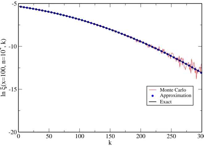
4 Logarithm of the probability for the site xto have receivedk visits after

n steps, lnξ(x, n, k), for x = 100 and n = 104_{, against k. Solid black}

line: exact value calculated by the expression at the beginning of this section. Blue points: Approximation 2.9. Solid red line: value obtained

by Monte Carlo method (mean over 104 _{realizations). . . . p. 23}

5 Function Ξ(n, x) versusx for three values of n. . . p. 24

6 Classification of 3D fixed points. The solutions to the determinant on the complex plane are shown in the left with a picture of the trajectories

near the fixed point on the right [3]. . . p. 27

7 Model for a fiber-reinforced composite (a) and a honeycomb structure

(b). The matrix phase is shown in gray. The fibers in (a) are indicated by white circles and the holes in the honeycomb (b) by black hexagons. The A and L directions correspond to loading in axial and lateral directions,

9 Schematic diagram of the computational model used in the simulations. (a) The chain of springs and binding sites are represented by small open circles. The two layers of sites surrounding the fiber are represented by

the big open circles and the two types of particles are shown as filled cir-cles with the red and blue circir-cles corresponding to the degradative and regenerative particles, respectively. A particle at the bottom, can move up, left or right whereas a particle at the top can move down, left, or

right. When a particle binds to a spring, it can stay there or move up or down. The ends of the chain are submitted to a constant forceF during the entire simulation. A periodic boundary condition was applied along the x direction. (b) A zoom into one of the springs representing collagen

monomers in parallel (black) reinforced by cross-links (gray). Red shows the force transmission pathways and the blue scissors represent a bound enzyme to a collagen monomer (middle diagram). Once the enzyme un-binds, the monomer is cleaved, but part of the monomer still participates

in force transmission. . . p. 45

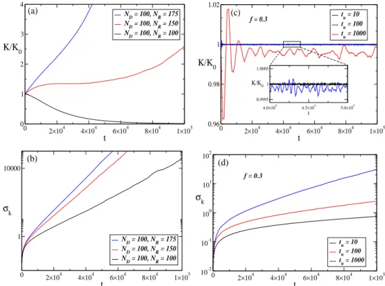
10 The normalized fiber stiffness and the standard deviation as a function of time. (a) The normalized stiffness K/K0, where K0 is the fiber stiffness

at t = 0, as a function of time when no regulation is applied. The number of D and R particles are indicated by ND and NR. (b) The

standard deviation σk of the local spring constants k as a function of time when there is no regulation. In panels (c) and (d), we show the normalized stiffness and the standard deviation as a function of time for the TCMmodel. In both cases, colors indicate different time periods tu at which the particles are updated to replace a fraction of them with new ones. The inset shows a close-up of the fiber stiffness for tu = 10 and 100. The parameters used in the simulations were: Ns = 103; γ = 0.995,

pof f = 0.5. These results were obtained from an average of 500 simulations. p. 46

11 Distribution of αi at different times (statistics accumulated over 500

deviation σk for three different applied forces F, when tu = 10 and f = 0.3. For all three values of F, a steady state is reached after which σk

displays only minor fluctuations. The inset showsnD andnR, the number of visits of degradative and regenerative particles to an individual spring. Differences in the number of visits of both types is always greater for

F = 10.0 than for F = 1.0. Panel 3b shows the standard deviation of

springs stiffnesses after the steady state, σs, is reached as a function of

F. The curve reaches a minimum for F _≈ 0.63 for all three values of

f. Panel 3c shows the mean spring stiffnesses after the steady state is reached as a function of F. The curve reaches a minimum for F _≈0.63

for all three values of f. These results were obtained from an average of

500 simulations. . . p. 48

13 Panel (a) shows the correlation function ξ(nD, nR) between the number of visits ofDandRparticles as a function of time for the models studied,

TCM and STCM. The correlation function is obtained by computing the correlation coefficient between two corresponding data series, the number ofD visits along the chain and the number of R visits along the chain. Panel (b) presents color maps of the average number of visits,nD and nR, to every spring along the chain at two time points for theTCM and STCM models. Blue and red represent low and high number of visits, respectively. The number of visits is normalized by the maximum number of visits at each time point. For the shorter diffusion time of

t = 103_{, the color maps forD andR particle visits are quite different for}

both models. For the longer time scale of t= 106_{, the color maps for the}

TCMremain different but the STCM displays perfectly matched color maps. This means that at each location, the number of visits of the two types of particle is the same balancing local digestion and repair. These

results are in agreement with the correlation function that approaches 1 only for theSTCM. These results were obtained from an average of 500

simulations. . . p. 49

14 Distribution of αi at different times (statistics accumulated over 500

highlighted parts in (b) are the segments selected for measurement of diameters along the axis of fibers. (c) presents the distribution of

diame-ters exhibiting a bi-modal shape. In (d) the diameters corresponding to each fiber are normalized by the median of the fiber (filled black circles). Note that the distribution now shows a single peak. Also shown are seve-ral model simulations of predicted diameter distributions corresponding

to 3 values of F in the STCM. Note that for F = 0.6, the simulated

distribution matches the experimental one. . . p. 51

16 (Upper) The “star” geometry. (Down) The “ring” geometry. . . p. 52

17 Effect of different number of layers (geometries star and ring) in the

STCM model. . . p. 52

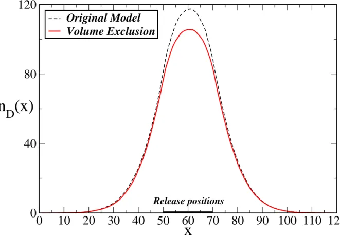
18 Average number of visits to sitex, when there’s no control and 20 parti-cles are released on the central sites as shown, after T = 103 _{time steps.}

These central sites are less visited than they are in original model.

Distri-butions obtained from 40,000 realizations in the model without control. p. 53

19 Average number of visits to site x, when there is no control and particles are released at random positions, after T = 103 _{time steps. All sites}

are less visited than they are in original model. Averages obtained from

40,000 realizations in the model without control. . . p. 54

20 The standard deviation σk as a function of time calculated considering the Volume Exclusion, for different geometries and number of layers in

the STCM model. . . p. 55

21 Infuence of the parameter f on the STCM. . . p. 56

22 Influence of pof f and pon on the number of bound and free particles.

Black: ratio between boundDparticles and freeDparticles as a function of time; Red: ratio between bound R particles and free R particles.

right and to the left isB. The probability of unbinding forR particles is

pon,R = 1−(1−pon,Lexp(−F/k)) so that pon,L is the probability to bind

to a spring with large stiffness. . . p. 58

24 Normalized fiber stiffnessKsand Standard deviation of spring stiffnesses

σs in the steady state as a function of γ in the STCM. Parameters used

were F = 1.0,tu = 100 and f = 0.3. . . p. 59

25 Standard deviation of spring stiffnesses whenD particles are sensitive to tension, but R particles are not. Here, the probability for a D particle to bind to a spring with stiffnessk ispon,D = ₁₊1_F/k. For R particles, the

probability was kept constant and equal to pon,R = 1₃. Parameters used

are F = 1.0,tu = 10 and f = 0.3. . . p. 60

26 Set of images obtained from the Scanning Electron Microscope. Fol-lowing the sequence of images, scale decreases from 100 µm until 100 nm

at the level where it is possible to identify the collagen fibers. . . p. 61

27 Collagen fibril diameter distributions during development of mice tendon

at 4 days (A), 10 days (B), 30 days (C) and 90 days (D). From Ezura

and collaborators [4]. . . p. 62

28 Bundle of collagen fibers (in white) after image treatment. Courtesy of

Hadler et al. . . p. 63

29 Electronic microscopy image of 3 weeks old mice tendon sample. The large structure in the middle is a tendon cell and the gray, nearly circular

objects are collagen fibers. Courtesy by Karl E. Kadler et collaborators. p. 66

30 Resultant image after the cell is omitted and the fibers are replaced by

ellipses of similar size. . . p. 67

31 Dispersion graph for radius versus average of neighbors’ radii for each

one of the 1452 identified fibers. There is no correlation, which means for example that it is not more probable for a large fiber to be surrounded

fiber stiffness k =x3. . . p. 69

33 Electronic microscopy image of 3 weeks old mice Achilles’ tendon sample.

Courtesy by Karl E. Kadler and collaborators. . . p. 70

34 Schematic representation for the evolution of the distribution function

n(r, t). The rate at which the number of particles enter the interval [a, b]

is G(a, t)n(a, t) and the rate at which they leave it is G(b, t)n(b, t). . . . p. 72

35 Left: Fragment of Fig. 5. Right: Representation of fibers by disks placed

randomly and whose size distribution comes from a bimodal distribution. p. 74

36 Collagen fibril diameter distributions during development of mice tendon at 4 days (A), 10 days (B), 30 days (C) and 90 days (D). From Ezura

and collaborators [4]. . . p. 76

37 Histograms obtained from Monte Carlo simulations for the population evolution. Growth, Birth and Fusion functions are G = are−γt

, B =

bδ(t−t0)N(r;µB, σB), K = 0. The parameters used here are a = 0.2,

γ = 0.09, b= 0.2,µB = 34.0,σB = 34.0, t0 = 5, µ0 = 30, σ0 = 10. . . . p. 77

38 Histograms obtained from Monte Carlo simulations for the population evolution. Growth, Birth and Fusion functions are G = are−_γt

, B =

be−βt

N(r;µB, σB), K = 0. Parameters: µ0 = 30, σ0 = 10, a = 0.2,

γ = 0.09, b= 0.2,β = 0.3, µB = 34, σB = 2. . . p. 78

39 Histograms obtained from Monte Carlo simulations for the population

evolution. Growth, Birth and Fusion functions are G = are−_γt , B =

be−_βt

N(r;µB, σB), Kij = Kp(i, j). The parameters used here are µ0 =

30, σ0 = 10, a= 0.2, γ = 0.1,b = 0.2,β = 0.3, µB = 34, σB = 2.0. The

calculated deviation function (see section 4.6) is ε= 66.0. . . p. 79

40 Deviation functionε, as defined in the text, for Monte Carlo simulations

with functions of growth, birth and fusion given by G = are−_γt , B =

be−_βt

N(r;µB, σB),Kij =Kp(i, j) and experimental data from Ezura et. all [4]. The parameters used here are σ0 = 10, a= 0.2,γ = 0.1,b= 0.2,

be−_βt

N(r;µB, σB), Kij = Kp(i, j). The parameters used here are µ0 =

40, σ0 = 10, a= 0.2, γ = 0.1, b= 0.2,β = 0.3,µB = 52.5, and σB = 2.0.

The values of µ0 and µB were obtained by the minimization method for the deviation function ε described in the text. For these parameters we

have ε= 13.1. . . p. 81

42 Stiffness, defined as K = P

i √_r

i, as function of time for three models

including only growth (G); growth and birth (GB) and growth, birth and

fusion (GBF). When present, the functions for growth, birth and fusion are G = are−_γt

, B = be−_βt

N(r;µB, σB), Kij = Kp(i, j). If applied, the parameters used here are µ0 = 30, σ0 = 10, a = 0.2, γ = 0.09, b = 0.2,

β = 0.27,µB = 34, and σB = 2.0. . . p. 81

43 Stiffness, defined as Φ = P

i1/ri, as function of time for three models including only growth (G); growth and birth (GB) and growth, birth and

fusion (GBF). When present, the functions for growth, birth and fusion are G = are−_γt

, B = be−_βt

N(r;µB, σB), Kij = Kp(i, j). If applied, the parameters used here are µ0 = 30, σ0 = 10, a = 0.2, γ = 0.09, b = 0.2,

Collagen is a generic name for the group of the most common proteins in mammals. It confers mechanical stability, strength and toughness to the tissues, in a large number of species. In this work we investigate two properties of collagen that explain in part the choice by natural selection of this substance as an essential building material. In the first study the property under investigation is the homeostasis of a single fiber, i.e., the main-tenance of its elastic properties under the action of collagen monomers that contribute to its stiffening and enzymes that digest it. The model used for this purpose is a one-dimensional chain of linearly elastic springs in series coupled with layers of sites. Particles representing monomers and enzymes can diffuse along these layers and interact with the springs according to specified rules. The predicted lognormal distribution for the local stiffness is compared to experimental data from electronic microscopy images and a good concordance is found. The second part of this work deals with the distribution of sizes among multiple collagen fibers, which is found to be bimodal, hypothetically because it leads to a compromise between stiffness and toughness of the bundle of fibers. We pro-pose a mechanism for the evolution of the fiber population which includes growth, fusion and birth of fibers and write a Population Balance Equation for that. By performing a parameter estimation over a set of Monte Carlo simulations, we determine the parameters that best fit the available data.

1

INTRODUCTION

Science of collagen has been progressing quickly in the last years and this is a reason

to celebrate. Its achievements include from anti-aging skin care products for cosmetic industry to tissue engineering, technological innovations that were not available only 40 years ago.

We know from daily experience that fibrous materials can be used to produce strong ropes to support high loadings or tissues with high or low elasticity, depending on the weaving. In a very similar way, collagen can be organized in many ways leading to a large

variety of mechanical properties [5]. This explains in part the versatility of collagen as a building material and justifies its abundance: collagen type I is the most common protein in mammals [1]. From an evolutionary point of view, we could say that it is a ”winner substance”. It appeared very early, soon after multicellular life started, and it has been

chosen by natural selection as the material that confers mechanical stability, strength and toughness to the tissues, in a large number of species [6].

Fig. 1 illustrates the assembly of collagen into tendon. It shows a complex hierarchical structure: at the lowest level, there are the collagen molecules, triple-helical protein chains with a length of about 300nm. Collagen molecules are further assembled by a parallel

staggering into fibrils which have a thickness in the range from 50 to a few hundred nanometers. Bundles of fibrils form thick, straight, parallel fascicles [7] with a thickness in order of hundreds of micrometers. Finally, fascicles perform tendon fibers, still at the scale of hundreds of micrometers. This is the scale we are looking at in this work.

Three important physical properties of materials are stiffness, strength and toughness and it is important to stress the difference between them. Stiff materials are defined

Figura 1: Sketch of the hierarchical of tendon. (a) shows some of the units, fiber, fascicle, fibril and molecule. (b) and (c) show detail of the interaction between fibrils and molecules, respectively. The proteoglycan-rich matrix between fibrils is indicated by PG. Extracted from [1].

reduced just by 1% while the overall strength is only half. The toughness of a material can be defined as the area under its stress-strain curve when it is loaded until failure.

Fig. 2 is a diagram that shows the approximate values of strength and stiffness for

several materials [2]. Such graph is sometimes referred to as an Ashby diagram[8]. Note that collagen based materials are placed in very diverse regions.

Mathematical modelling of collagenous materials contributes by making an effort to reduce this extremely complex biological system into simple models that can be treated with the apparatus offered for example by Nonlinear Dynamics and Mechanics.

In this work we propose two models to study different characteristics of collagen fibers. The first one deals with a single fiber and the second, with a population of fibers. The

work is organized as follows.

The second chapter is an overview about very diverse topics that will be used or

refered to in what follows. It includes the minimum necessary theory of mathematics of diffusion, nonlinear dynamics systems, stiffness and toughness of materials and image processing.

Figura 2: Ashby plot of the specific values (that is, normalized by density) of strength and stiffness (or Young’s modulus) for both natural and synthetic materials[2]. Note the spread values for collagen-based materials (in pink).

diffuse and alter the springs’ local stiffnesses. These particles represent enzymes capable of digesting them and collagen monomers that repair them.

The fourth chapter contains our discription of the populational dynamics for a bunch of collagen fibers. It is known that the distribution of size of these populations present two characteristic peaks, but a mathematical model that includes the three main mechanisms that matter - growth, fusion and release of new particles - and explains the observed

2

FUNDAMENTALS

2.1

Random Walk and Diffusion

When a collection of particles such as cells, bacteria, chemicals, animals and so on, move around in a random way, the particles spread out as a result of this irregular individual motion. When this microscopic irregular movement results in some macroscopic or gross regular motion of the group it can be called adiffusion process.

2.1.1

Displacement in a 1D Random Walk

Among the simple models used in Physics, the Brownian motion is one of the most

known. Its development was motivated by a biological phenomenon, namely the motion of particles trapped in cavities inside pollen grains in water observed first for Robert Brown in 1827 [9]. A problem closely related to Brownian motion is that of a “random walker”. This idea was proposed by Karl Pearson in a letter to Nature in 1905 and goes as follows.

A man starts from a point 0 and walkslyards in a straight line; he then turns through any angle whatever and walks anotherl yards in a straight line. He repeats this process

N times. What is the probability that after these N steps he is at a distance between r

and r+δr from his starting point?

Let us consider the one-dimensional isotropic version of the random walker problem. A walker is at position 0 initially. It can sit at regularly spaced positions along a line that are a distance ∆xapart so we can label the positions by the set of integersm. After fixed

times intervals ∆t the walker either steps to the right with probability p= 1/2 or to the left also with probabilityq = 1/2. Our aim is to obtain the probability p(m, N) that the walker will be at positionm after N steps.

There are many ways to start at x = 0 an go through N steps to nearest-neighbour sites and end up at x= m. The walker must have made n1 =m+n2 steps to the right

steps to the right and n2 = 1₂(N −m) steps to the left. The probability for making n1

steps to the right and n2 steps to the left is

1 2 n1 × 1 2 n2 = 1 2 N

And the number of ways to have n1 steps to the right and n2 to the left is

N!

n1n2

= N!

n1!(N −n1)!

Therefore the probability of being at position x=m after N steps is

p(m, N) = N!

n!(N ₋n)!

1 2 N = N n 1 2 N . (2.1)

We are interested on the behaviour of the binomial distribution for long times, i.e. for

N → ∞. Assuming N ≫1 we can use Stirling’s formula to approximate the factorials:

lnN! =

N +1 2

lnN −N+ 1

2ln 2π+O

1

N

(2.2)

From this we get

lnp(m, N) =

N +1 2

lnN₋

N +m

2 +

1 2

lnN+m

2 −

N ₋m

2 +

1 2

N ₋m

2 −Nln 2− 1 2ln 2π (2.3)

which is equivalent to

p(m, N)_→ p 2

2πσ2

m exp

−1₂(dm)

2

σ2

m

(2.4)

whereµ and σ2 _{are respectively the mean and variance of p.}

We can perform a continuous limit and introduce x = m∆t, t = N∆t, D = 1₂(∆_∆x_t)2, finding then

p(m∆x, N∆t) = p 2

2πσ2

m exp

−1_22Dtx

. (2.5)

In the limit ∆x → 0, ∆t → 0, D = const., we find the probability density to find the walker in an interval (x, x+dx) as

p(x, t) = √ 1

4πDtexp

− x

4Dt

, (2.6)

2.1.2

Number of visits in a Random Walk

For reasons that will become clear in the next chapter of this work, it is important to study the number of visits of a random walker to the sites of a linear chain.

The number of visits that some site at positionxhas received afternsteps depends, of

course, on the whole history of the walker. In the Fig. 3 we show the 2n _{possible histories} for a walker that starts at the positionx= 5, forn = 0,1,2,3,4. We label each one of the 2n _{possibilities by an index j = 1, ...,2}n _{and define a row matrix P}

j(n) whose i-th entry is the number of visits that the siteihas received after n steps, if the walker has followed

the path j. Note that for each path j there are two possibilities for the position of the walker. By the labeling system we used in Fig. 3, this means that

Let ξ(x, n, k) be the probability for the site x to have received k visits after n steps. Then, for anyk = 1,2, ..

ξ(x, n, k) =

       1 2n−k+1

n−k+ 1 (n+x)/2

if n+xis even

1 2n−k

n−k

(n+x₋1)/2

if n+xis odd

as has been proven by R´ev´esz [10] who calls the function ξ(x, n, k) the local time for the Random Walk.

R´ev´esz also shows that, for k = 0, x= 0 we have:

ξ(x, n,0) = 1₋2−n n

X

j=x

n

[(n−j)/2]

Taking the logarithm on both sides of the equation for n+x even andk > 0, and we have

lnξ(x, n, k) = (₋n+k₋1) ln 2 + ln(n₋k+ 1)!₋ln

n₋k+ 1₋ n+x 2

!₋ln

n+x

2

!.

(2.7) Let us study the behaviour of this function for large n. Using Stirling’s formula 2.2 to

Figura 3: Possibilities for a one-dimensional random walk aftern= 4 steps. The number of visits every site has received is indicated by means of the vector~p. The number of visits for the central cite x = 0 is in red. The blue circles indicate the possibility for reaching the same final state through different paths.

introducing the abbreviationsh_≡ n−_x

2 and m≡

n+x

2 we get:

lnξ(x, n, k)≈(−n+k−1) ln 2 + (n−k+ 3

2) ln(n−k+ 1)−

n−k−m+ 3 2

ln(n−k−m+ 1)

−

m+1 2

−n+k+m₋1₋ 1 2ln 2π

(2.8)

If now we use the expansion of logarithm:

ln(1_±x) = _±x₋1

2x

2_+O(x3₎

we conclude that if some factorX is much smaller than N, N ≫X, we have:

ln(N ±X) = lnN

1±X

N

= lnN ±X

N − 1 2 X N 2 +O X N 3

Considering thatn+1_≫kandn₋m+1_≫kand making successivelyN =n+1;X =

0

50

100

150

200

250

300

k

-20

-15

-10

-5

ln

ξ

(x=100, n=10

4

, k)

Monte Carlo Approximation Exact

Figura 4: Logarithm of the probability for the sitexto have receivedkvisits afternsteps, lnξ(x, n, k), for x = 100 and n = 104_{, againstk. Solid black line: exact value calculated}

by the expression at the beginning of this section. Blue points: Approximation 2.9. Solid red line: value obtained by Monte Carlo method (mean over 104 _{realizations).}

powers onk to finally arrive at

lnξ=A+Bk+Ck2 (2.9)

where

A=₋(n+1) ln 2+(n+3/2) ln(n+1)₋(m+1/2) lnm₋(1/2) ln(2π)₋(n₋m+3/2) ln(n₋m+1);

(2.10)

B = ln

n+ 1 2(n₋m+ 1)

(2.11)

C = 1 2

m

(n+ 1)(n₋m+ 1) (2.12)

-400

-200

0

200

400

x

0

2000

4000

6000

8000

Ξ

(n,x)

n = 1000

n = 5000

n = 10000

Figura 5: Function Ξ(n, x) versus x for three values of n.

n steps, that we will approximate by an integral Ξ(x, n) defined by

Ξ(x, n)≡ lim a→₀

Z ∞

a

ξ(x, n, k)kdk. (2.13)

Using the definite integral

Z ∞

0

kea−_bk−_ck2

dk = e a

4c3/2

2√c−√πbeb2/4cerfc

b

2√c

(2.14)

we get

Ξ(x, n) = e a

4c3/2

2c1/2₋√πbeb2/4cerfc

b

2√c

(2.15)

wherea=A, b=−B, c=−C.

For reasons that will be apparent in the next chapter, we are interested in the variance of Ξ(x, n) over the position, i.e., in the quantity

σ_x2(n)≡Var[Ξ(x, n)] =

Z ∞

0

Ξ(n, x)x2dx−

Z ∞

0

Ξ(n, x)xdx

2

. (2.16)

result: In a simple random walk, the standard deviation of the number of visits among the visited sites after n steps scales according to tν_{, withν ≈0.7.}

2.2

Three-dimensional nonlinear dynamic systems

Stability of systems of ordinary differential equation such as arise in interacting po-pulation models and reaction kinetic systems is determined by the roots of a polynomial.

The stability analysis we are concerned with involves linear systems of the vector form

d~x

dt =A~x, (2.17)

or, more explicitly,

˙

x1 =f1(x1, x2, x3);

˙

x2 =f2(x1, x2, x3);

˙

x3 =f3(x1, x2, x3).

The so-called Jacobian matrix of this system is given by

J = ∂f1 ∂x1 ∂f1 ∂x2 ∂f1 ∂x3 ∂f2 ∂x1 ∂f2 ∂x2 ∂f2 ∂x3 ∂f3 ∂x1 ∂f3 ∂x2 ∂f3 ∂x3

and the “characteristic polynomial” is

|J −λI_|= 0, (2.18)

whereI is the identity matrix. This equation leads to a cubic equation

λ3+a1λ2+a2λ+a3 = 0. (2.19)

The solution ~x = 0 is stable if all the roots λ of the characteristic polynomial lie in the left-hand complex plane, that is Re(λ) < 0 for all roots λ. If this holds then ~x _→ 0 exponentially ast _→0 and hence~x= 0 is stable to small perturbations.

One can find conditions on the ai, i = 1,2,3, such that the zeros of P(λ) have

a1 >0; (2.20)

a3 >0; (2.21)

a1a2−a3 >0. (2.22)

We should mention the other possibilities besides Re(λ) < 0 for all λi. The fixed points are classified according to the signs of the real and imaginary parts of the three

characteristic values, the solutions of equation 2.19. Specifically:

Characteristic values Fixed point

(−, −, −) Attracting node (−, −r+ia, −r−ia) Stable spiral

(+, +, +) Repellor

(+, +r+ia, +r₋ia) Unstable spiral

(−, −, +) Saddle point index 1 (−, +, +) Saddle point index 2 (₋r+ia, ₋r-ia, +) Spiral saddle index 1 (₋, +r+ia, +r-ia) Spiral saddle index 2

The behavior of trajectories near the fixed point is illustrated in Fig. 6.

2.3

Stiffness and toughness of materials

For most biological materials (Wainwright 1982) the internal architecture determines the mechanical behavior more than the chemical composition does. To illustrate this fact, Fratz [1] considers these two simple examples: a composite of stiff fibers in a soft matrix

and a honeycomb structure. Using the Voigt and the Reuss model for a fiber composite as sketched in Fig. 1.1a (Hull and Clyne 1996), where the volume fraction of the matrix phase is called Φ, the elastic young modulus in axial and lateral directions are given as a function of the modulesEm and Ef of matrix and fibers, respectively, by

EA= ΦEm+ (1−Φ)Ef and EL= (ΦE −₁

m + (1−Φ)E

−₁

f )

−₁

sketched in Fig. 1.1b, the elastic modules in axial and lateral directions, respectively, can be estimated to be (Gibson and Ashby 1999)

EA/Em ∝Φ and EL/Em ∝Φ3

Again, with thin walls in the honeycomb structure (that is, Φ_≪1), the difference between

lateral and axial mechanical properties can be orders of magnitude. These two examples show that by simple structuring, mechanical properties can vary enor- mously, even though the chemical composition is the same. In particular, the local fiber orientation plays a major role for adapting the mechanical properties of most biological materials.

Figura 7: Model for a fiber-reinforced composite (a) and a honeycomb structure (b). The matrix phase is shown in gray. The fibers in (a) are indicated by white circles and the holes in the honeycomb (b) by black hexagons. The A and L directions correspond to loading in axial and lateral directions, respectively [1].

2.4

Image processing

A grey-scale two dimensional image is stored in a computer by a matrix, each entry of which (apixel) is a value that can take values from a scale that goes for example, from 0 (for black) to 255 (for white). The treatment of images using mathematical operations

over their components is called Image Processing [12].

In this work we used image processing techniques to isolate the images of the collagen fibers and obtain informations about them, mainly their diameters. In what follows we discuss briefly the technique that we used for detecting the borders of the fibers.

Detection of borders is based on the difference of brightness between neighbor pixels. A sample of image from electronic microscopy is shown in Fig. 8a. Although fibers can be seen clearly with the naked eye, the image is very noisy, with the presence of pixels

to reduce the noise we apply a Gaussian smoothing. Each pixel’s new value is set to a weighted average of that pixel’s neighborhood. Specifically, a mathematical process called convolution is used. The convolution of a filterh(m, n) and an imagea(m, n) generates a new imagec(m, n) which can be written as follows:

c(m, n) = a(m, n)∗h(m, n) = r

X

j=0

s

X

k=0

h(j, k)a(m−j, n−k) (2.23)

In the case of the Gaussian filter, the convolution kernel is

h(m, n) = e−

_m2₊n2

2σ2

(2.24)

where the parameter σ controls the extent of smoothing. Fig. 8b shows the result of Gaussian smoothing to the original image (withσ = 2).

Figura 8: Procedure for detecting the borders of collagen fibers: A. Original Image; B. Application of a Gaussian filter; C. Thresholding; D. Edge detection.

white while the others are set to black. Fig. 8cshows the result of this operation applied to 8b. Here, the intensity threshold was chosen to be 0.55 of the maximum intensity.

Finally, we obtain the gradient image by assigning a larger value of intensity nearer to the white contour to the pixel point where the gradient value is greater than a certain threshold, keeping all other points unchanged, that is,

g(x, y) =

 



b if _|∇f(x, y)_{| ≤}τ

f(x, y) else.

Fig. 8d shows the result of the gradient operation to the image 8c.

If f(x, y) is an image function, the gradient at the pixel point (x, y) is defined as the

vector

∇f =

∂f ∂x, ∂f ∂y (2.25)

and the direction of the gradient is defined as

θ(x, y) = arctan ∂f ∂y ∂f ∂x ! (2.26)

whereθ(x, y) denotes the angle between the gradient direction and thex-coordinate. The magnitude of the gradient may be defined as

|∇f_|=

s ∂f ∂x 2 + ∂f ∂y 2 (2.27)

Different methods may be applied to approximate partial derivatives. For example, we can use the first-order forward difference to approximate the gradient as

∂f

∂x(i, j)≈f(i+ 1, j)−f(i, j) (2.28)

and

∂f

∂y(i, j)≈f(i, j+ 1)−f(i, j). (2.29)

Of course the gradient of a pixel is related to every pixel point in its neighbourhood while those formulae take into account only two of its neighbours. So in practice some

∂f

∂x and

∂f

∂y by using the following operators:

hx = 1 8



  

+1 +2 +1

+2 0 0

+1 −2 −1



  ∗

A

hy =



  

+1 0 ₋1

+2 0 −2 +1 0 −1



  ∗

A.

Although it is important to understand the mathematical details involved in the image processing, in practice there are many softwares that allow the user to apply those

3

A MODEL FOR

HOMEOSTHASIS OF

COLLAGEN FIBERS

3.1

Introduction

The extracellular matrix (ECM) plays a role in tissue development, damage re-pair, diseases and aging by influencing cellular responses. For example, the stiffness of the substratum on which stem cells are cultured has been found to direct cellular

diffe-rentiation [13]. On the other hand, cells sense the mechanical properties of theECM as well as secrete ECM components [14]. This mutual dependence between the ECM and its embedded cells likely evolved soon after multicellular life emerged on Earth [15].

Cellular maintenance of theECMrequires an effective regulation that balances enzy-matic degradation with replacement of the digested fragments with newly synthesized

molecules forming and shaping the fibrils and fibers of the ECM including collagen and elastin. In several organs and tissues such as the vasculature, skin, heart and periodon-tium, a quick turnover of collagen with half-lives between 20 and 250 days have been observed [16, 17]. Additionally, the mechanical stresses imposed by exercise are known

to induce rapid and significant collagen turnover within 72 hours even in tendon [18], which has a very long turnover of collagen [19].

Despite the strong and constant cellular maintenance, the micro-structure of collagen appears to remain in a stable homeostatic state throughout most of adult life even when demanding mechanical stresses lead to incessant remodeling. For example, while the diameter distribution of collagen in mouse tail tendon undergoes major changes until

the age of 3 months due to development, the distribution remains nearly independent of age between 4 and 23 months [20], a range that spans the adult life of the mouse and corresponds to approximately 10 to 60 years of human life [21]. Similarly, collagen

consequence of the nearly constant diameter distribution is a stable strain energy density that maintains proper mechanical function and resistance to rupture during this time period [20]. These findings raise an important question in mechanobiology: “How are cells able to maintain such a homeostatic structure over a period that corresponds to

decades of human life?” While several studies have reported on the details of short-term ECM maintenance [14] and collagen biosynthesis [23], much less is known about the truely long-term regulation of ECM composition and structure. It appears that some as yet unknown control mechanism regulates the maintenance of ECM structure throughout much of adult life until this mechanism eventually loses its efficiency due to aging as evidenced by the increasing irregularity of the collagen fiber structure [24, 25].

3.1.1

Basic Model Formulation

To study how cells can balance enzymatic digestion and repair of a collagen fiber, we use a random walk model to mimic the diffusion along the fiber of two different

types of molecular complex, which we refer to as regenerative (R) and degradative (D) particles. The R and D particles representing collagen monomers and collagen-cleaving enzymes such as matrix metalloproteinases, respectively, carry out the local fiber repair and digestion. The fiber consists of a one-dimensional chain of Ns linearly elastic springs

in series (Fig.1a). The fiber is surrounded by two layers of sites along which the R and

D particles can diffuse and bind to the fiber at discrete locations corresponding to the springs. Periodic boundary conditions are applied in the x direction. Both ends of the chain are subject to a constant force that mimics tension on ECM fibers. To simulate the digestion and repair activity along the fiber, we begin with a chain having identical initial spring constants k(t = 0)≡k0.

The particle diffusion is initiated by releasing a set of particles of both types at random positions in the two layers surrounding the chain. The number of particles corresponding to the two types, NR and ND, is initially fixed at time t = 0. Additionally, the particles

do not interact with each other and there is no exclusion principle, which means that

particles can simultaneously be at the same position surrounding the chain. However, only one particle is allowed to bind to any given binding site.

To carry out fiber maintenance, we apply the following rules to the diffusion and reaction processes depending on the type of particle:

associated with diffusion;

2. The probability for a particle to move up from the bottom layer or move down from the top layer is pon. This step represents the event that a D or a R particle binds

to the fiber. The specific rules that govern the binding processes depend on the

model considered (see below) and the particle type. For D particles, the diffusion and binding processes are similar in the sense of probability resulting in an isotropic diffusion for all models considered. For Rparticles, the binding process depends on the specific model used and the process can be isotropic or anisotropic;

3. The probability for a bound particle of either type to leave the fiber and move up to the top layer or move down to the bottom layer is poff. This parameter controls

the unbinding process and is associated with repair or degradation;

When a D or an R particle unbinds, the local spring constant k is reduced (k_→γk)

or increased (k → k/γ), respectively, by a constant factor γ. The reason for this is as follows. The fiber is composed of molecules in parallel and series. If the fiber was a regular array of molecules, cleavage would decrease the number of molecules in parallel. This would result in a linear decrease in the spring constant during subsequent cleavages

and over a long time scale, it becomes possible that the local spring constant reaches zero effectively rupturing the chain. In reality, the molecules overlap and are connected via multiple inter-molecular as well as inter-fibril cross-links in a complex manner (Fig.1b). Hence, the degradation of the fiber is also a complex process and a single cleaving event

does not necessarily have to eliminate a complete monomer from the chain. Indeed, Fig.1b

demonstrates that following the cleavage of a monomer, part of the same monomer can still carry a force. Due to this complexity, simply subtracting one unit fromkfollowing an unbinding of aDparticle is not appropriate. Therefore, we model the cleavage process by

assuming that the decrease in spring constant is proportional to the actual value, which corresponds to a multiplicative degradation process. This assumes that the process of degradation is far away from the rupture threshold and this model provided an accurate description of stress relaxation and fragment release from elastin fibers [26].

3.2

Time Controlled Regulation of Fiber Maintenance

actively measuring the stiffness of their surrounding matrix [27, 28] and respond by secreting degradative enzymes [29] or upregulating enzyme inhibitors and eventually collagen production [30]. To mimic this behavior, the stiffness of the fiber is periodically evaluated at time intervals tu. If the stiffness is impaired (K < K0), a fraction f of the

particles are randomly selected to be relabeled asRparticles. Alternatively, if the stiffness is too high (K > K0), the same fraction f of the particles are randomly chosen to be

relabeled as D particles. It is important to note that during this relabeling process the system does not recognize the particle type to be relabeled. However, statistically, this

replacement process mimicking cellular response to alterations in fiber stiffness is able to change the overall concentration of particles around the fiber so as to regulate the overall maintenance process to be degradative or regenerative if the fiber is too stiff or too soft, respectively.

It is possible to define the periodic control in many ways. For example, the

stiff-ness of the fiber can be checked at every time step and relabeling particles can be based on whether K surpasses a predefined threshold below or above the target K0. We find,

however, that such details about how the control is performed do not influence the general behavior of the system. Nevertheless, the presence of some periodic control is

fundamen-tal. If it was absent, it would be impossible for the fiber stiffness K to reach a steady state value, even if the number of particles of both types is always the same. The reason is that K is the harmonic mean of individual spring stiffnesses which introduces strong nonlinearity in the model with a tendency to decrease the overall fiber stiffness. Note, for

example, that if one spring binds aDparticle whereas another spring of the same stiffness binds an R particle, the two events do not compensate each other and the overall effect is to reduceK. To see this, consider the change in stiffness:

∆(K−₁ ) = 1

γk +

1

k/γ −

1

k +

1

k

>0_⇒∆K <0. (3.1)

In order to maintain proper functionality, the cellular maintenance of a fiber needs to

preserve the fiber’s elastic properties within a narrow target range. While a simple random walk model without control cannot achieve this, the TCM produces a stationary K. However, theTCMis unable to produce a homogeneous fiber since the standard deviation of fiber stiffness, σk, diverges as shown in Fig.10(d). The reason for the divergence is the

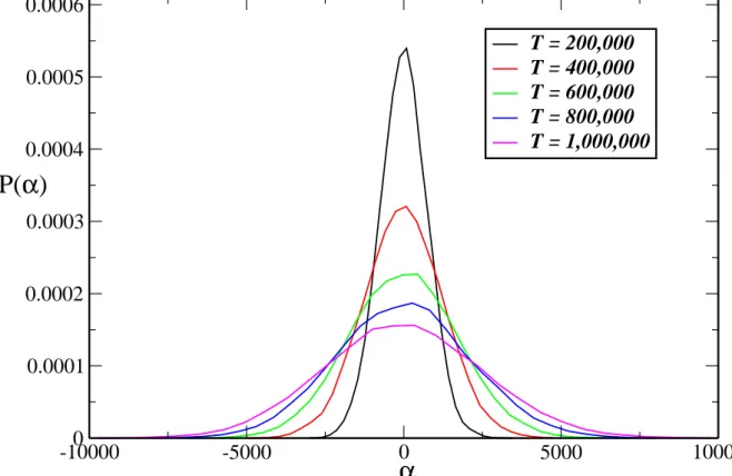
simple random walker is proportional totν _{withν = 0.5, in our simulations the standard} deviation for the distribution ofα _∼logk varies according toσ_∼tν _{with ν≈0.7. Hereα} is simply the difference between the number of visits ofD and R particles a given spring has received. To emphasize the similarity between TCM and the random walker model we show in Fig. 11 the distribution ofα at five different time points. As we can confirm the distribution is very similar to one obtain in the random walker model, but with a different exponentν.

Tabela 1: Summary of model parameters and measured quantities.

K(t)/K0 Normalized stiffness of the fiber at instant t .

σk Standard deviation of local spring stiffnesses . hksi Mean of springs stiffnesses in the steady state.

σs Standard deviation of springs stiffnesses in the steady state.

ND, NR Number of D and R particles in the system. The sum ND +NR= 100 is kept constant.

tu Time period of updating particle types.

f Fraction of particles relabeled at each update event.

F Force applied to the fiber per unit of length.

pon,D, pon,R Probabilities of binding for D and R particles.

While pon,D = 1/3 is kept constant, pon,R depends on F as show in (Eq. 3.2).

pof f Probability of unbinding.

3.2.1

Spatio-temporal Control of Fiber Maintenance

To control both the mean and homogeneity of fiber stiffness, we introduce an addi-tional feature in the model, the local control of the binding event based on the observation that the absence of tension on the ECM leads to disorganized fibers [31]. This new in-gredient is expected to introduce an anisotropy in the diffusion-reaction process making

the weaker springs more susceptible to be visited by R particles. We call this model

spatio-temporal control model (STCM). While the behavior of the D particles remains the same as in the TCM, the probability pon,R for an R particle to bind to the fiber now depends on the local stiffness with spring constantk as follows:

pon,R = 1− 2 3e

−_F/k

, (3.2)

generates a higher local stretch. We assume that a higher local stretch unfolds cryptic binding sites [34, 35]. Thus, depending on the local stiffness k, pon,R can vary along the chain with higher values at regions where the fiber is weaker due to more frequent visits of D particles. Consequently, since pon,R is higher at such locations, R particles tend to

visit these sites with a higher probability. However, as soon as the R particles start to increasek,pon,R naturally decreases recovering a value which corresponds to the isotropic diffusion-reaction case.

During the digestion/repair processesF is assumed to be constant butkalong the fiber shows substantial heterogeneity, as we have confirmed by the divergence in σk for both

the random walk model without control and theTCM. To test whether theSTCM can control the global elasticity while preserving fiber homogeneity, we carry out simulations with the STCM for different values of f and tu. We also examine the effect of F by varying it between 0.04 and 10. For all cases, the global fiber stiffness K is well controlled

as in the TCM. However, σk no longer diverges. The main plot in Fig.3a shows indeed that σk reaches a steady state although its value σs depends on F. Here, σs is the value around whichσk fluctuates after it has reached a steady state.

Next, we run a set of simulations with various combinations of the parameters F, tu and f in the STCM. For all parameter combinations, σk always reaches a steady state with σs depending on the actual parameters. We plot σs as a function of F for fixed

tu = 10 and three values of the fraction f in Fig.3b. Surprisingly, σs presents a minimum as a function ofF that occurs at F _≈0.63. The maximum homogeneity of stiffness along the fiber is thus achieved when σs is minimum which depends on the applied force as

well as the strength of cellular control modeled by the fraction of particles f replaced during the fiber maintenance process. The decrease in σs for larger values of f results from the stronger and more effective feedback to regulate global stiffness through a higher concentration of control particles in the system. The presence of a minimum can be

explained by recalling that the process of degradation and repair is similar to a random walk whenF = 0 which results in a divergence ofσk. For any small positive value ofF, the local control results in finite σk and with increasing F, the control becomes stronger and

σk decreases. However, when F further increases, the control of the R particles becomes

much faster than that of D particles leading to overshoots in repair and a subsequent increase in σk which we have verified by examining the local time variation of individual springs (not shown). Similarly to σs, the mean fiber stiffness also shows a minimum for

F _≈ 0.63 (Fig.3c). For the strongest control when f = 0.9, the fiber stiffness is close to

forRand Dparticles increases making the Rparticles more effective and increasing fiber stiffness.

3.2.2

Analysis of Fiber Maintenance by the STCM

Both the TCM and STCM models presented here are able to regulate the fiber stiffness within an interval less than 5% of its initial value over time. However, only

theSTCM can regulate the standard deviation of the stiffness along the fiber. To better understand how theSTCMachieves this level of control, we performed a simple analytical calculation to shed light on the conditions which must be satisfied in order to obtain a constantσk. At any instant, the value of each spring constant is the product of the initial

value at t = 0 and γnD−_nR

, where nD −nR is the difference in the number of visits of the two types of particles and γ is constant. For many realizations, the distributions of the number of visits, p(nD) and p(nR), approach a Gaussian distribution at any instant in time. It can be shown that the distribution of α=nD−nR, which determines k, also

approaches a Gaussian as shows in Figs. 11 and 14 with a variance given by

σ_α2 =σ_n2D+σ

2

nR −2ξ(nD, nR)σnDσnR, (3.3)

whereξis the correlation function betweennD and nR. Thus, k of a single spring is given byγα_k

0, and at each instant in time, the distribution ofk approaches a lognormal with a

variance given by

σ2_k = exp (lnγ)2σ2_α+ 2(lnγ)µα

exp (lnγ)2σ2_α

−1

. (3.4)

Forσ2

k to reach a steady state in theSTCM, the following two conditions must be met: (i) dσ2

α/dt = 0 and (ii) dµα/dt = 0. Examining Eq. 3.3, it can be seen that the first condition is satisfied if (dσnD/dt=dσnR/dt) and the correlation function ξ(nD, nR) = 1.

Condition (ii) is equivalent to dµnD/dt = dµnR/dt, i.e., the two types of particle should

visit springs at the same rate.

The conditions obtained above are confirmed by the simulation results in Fig.4a.

The correlation function ξ(nR, nD) reaches and slightly fluctuates near unity only for the

STCM. To corroborate that the average number of visits has the same value for both the D and R particles, we plot in Fig.4b color maps of the average number of visits per spring for both particles along the chain for short and long time scales, t = 103 _and

which is in agreement with the calculations in the case of STCM. Thus, the STCM as a model of biological regulation of fiber maintenance fulfills the requirement to keep both elasticity and homogeneity of a fiber within a narrow range in the presence of continuous degradation and repair. This can be achieved only in the presence of tension on the fiber

which places part of the regulatory mechanism outside the cell because the binding affinity becomes a function of the applied force as well as the local stiffness along the fiber.

3.3

Comparison of Model Prediction to

Experimen-tal data

Comparison of our results with experimental data would require measurements of the variation of the Young’s modulus of individual collagen fibrils along its axis. To our

knowledge, no such Young’s modulus measurements in the axial direction are available along the collagen fibers. Atomic Force Microscopy measurements along the fibril in indentation mode showed significant axial heterogeneity of stiffness [36]; however, the indentation induces both compression and shear and since collagen is anisotropic with

different axial and lateral moduli, such data are not directly applicable to estimate the Young’s modulus in axial extension. Nevertheless, a positive correlation between average fiber diameter and the low strain modulus has been found for artificial assemblies of type I collagen fibers [37]. To extend this to a relation between local diameter and local stiffness,

we note that the stiffness at any given location should be related to the number of collagen monomers Nc that pass the cross sectionA of the fiber. If we assume that the cross-link density is constant along the fiber, the local stiffness should be proportional toNc. Since

A is the sum of the cross sectional areas of individual monomers, A is also proportional

to Nc implying that fiber diameter is proportional to the square root of Nc. Thus, we compute the distribution ofk1/2 _{and compare it with the distribution of diameters along}

individual collagen fibrils.

Images of the thoracic aorta of normal rats were obtained by scanning electronic microscopy (Fig 5a). After image processing, segments were selected if their borders could be identified properly using an edge detection method. A set of 165 segments were

included in the final analysis. The results of this process are shown in Fig. 5b. The distribution of diameters exhibits two peaks (Fig. 5c) similar to recent results obtained by measuring cross sectional areas on images perpendicular to the fiber axis [20]. We next normalize each diameter value along a fiber with the corresponding median diameter so as

is compared to the distributions of k1/2 _{for 3 values of F in Fig. 5d. We find a good}

match between our experimental results and the model simulations with F = 0.6, which corresponds to the minimum of σs in Fig. 3b or the maximum homogeneity of the fiber. Note that no formal fitting of the model was carried out to fit the data. Also, both the

experimental and the model predicted diameter distributions are nearly Gaussian with a narrow variability of 13% around the mean.

3.4

Discussion

In this study, we investigated the cellular long-term maintenance of an elastic fiber under tension including degradation and repair processes combined with diffusion

of regenerative and degradative particles by various computational models. Our main finding is that a homeostatic fiber stiffness can be achieved easily by assuming that cells periodically probe the overall stiffness of the fiber and properly adjust the production and release of degradative enzymes and regenerative monomers. However, this control

mechanism fails to maintain a homogeneous fiber that can be seen on images of collagenous tissues. We also introduced the idea that part of the control mechanism is locally governed by how the biophysical properties of the fibers including binding affinity are modulated by the applied force on the fiber. This model predicts diameter variations along the fiber

that are in quantitative agreement with experimental data when the applied force is in the range where the variance of local stiffness is at its minimum. Thus, our model predicts a strong involvement of the fibers in their own repair that warrants further experimental studies. While little is known about how tensile forces regulate fiber repair [31], more

studies reported regulation of ECM degradation by mechanical forces [38, 26, 35, 39, 40]. The combined regulation of both repair and digestion by mechanical forces can be studied computationally; however, it needs to be tested experimentally how the on rate of the regenerative particles changes with mechanical forces on the fibers.

Various computational models have been developed to describe tissue remodeling and

homeostasis [41, 42, 43]. However, to our knowledge, our model is unique in that it investigates the combined effects of diffusion and binding of two different particles on the long-term homeostatic structure and function of fibers. An interesting result of the simu-lations is that cellular control of long-term fiber maintenance is possible only when tension

can be regulated by mechanical forces to achieve a minimum value. Furthermore, these fiber properties are not independent of each other as they are both a consequence of the axial distribution of stiffness. This represent an important structure-function relation for the fiber which may offer a way to control fiber and tissue mechanical properties through

the different pre-existing mechanical stresses in various organs. Indeed, the transpulmo-nary pressure in the lung is between 0.5 and 1 kPa [44] whereas the transmural pressure in arteries is around 10₋15 kPa [45]. This is another prediction of the model that can be tested experimentally.

Our model also has limitations. First, the model is 2-dimensional while the diffusion

of particles in the ECM occurs in 3 dimensions. We tested the influence of adding 5 layers in a star-shape configuration as show in Fig. 16 (U pper) in which the diffusing particle can step left, right or onto the fiber, but not directly from one layer to another. However, when the particle unbinds, it can step onto any of the five layers. We find that

the distribution of α is the same in the 2-layer and 5-layer models. We also test another model, called the ring configuration (see Fig. 16 (Down)), in which the diffusing particle is allowed to step left, right, onto the fiber as well as across the layers. Again, the number of layers does not matter; however, in this case, the distribution of α as well as σk are

different from those in the star configuration as we can confirm base on results present in Fig. 17. The reason is that in the ring configuration, the diffusing particle can spend more time around a single binding site and this is similar to adding a waiting time to the diffusion that changes the axial diffusion constant. Consequently, the particle can step

onto the same binding time more often and generate stronger heterogeneity ofk along the fiber. Another limitation is that two particles can step on the same site during diffusion. When we include volume exclusion not only on the fiber but also on the diffusion sites, the dynamics of the control becomes slightly slower because the number of visits at a

given site is slightly reduced (see comparison between both cases in Figs. 18 and 19). The introduction of volume exclusion also leads to the number of diffusion layers becoming a small factor in the steady state of the of the variance as we confirm base on results show in Fig. 20. With respect to the periodic assessment of fiber stiffness we note the

following. The fraction f of particles relabeled as R or D, f affects the average stiffness (Fig. 12c) showing a minimum around F = 0.6 but not the steady state numbers of R

and D particles around the fiber which are determined by the on and off rates. Thus, f

can be considered as the strength of cellular control and hence it represents an effective

turnover rate of collagen.

out further simulations. The number of particles in the system fluctuates around the proportion of roughly 60% D particles and 40% R particles for all values of f, but the amplitude of the fluctuations are greater for largerf. Thus, a stronger control via repla-cing more particles when needed implies a faster convergence to steady state lowering its

value as indicated in Fig. 12(b). In Fig. 21, we show the time variation of the number of D and R particles in the system for three values of f. The probabilities pon and pof f are the parameters that actually control the steady state concentration of particles in the system. In order to see how the number of particles typeDand Rfluctuate as a function

of the probabilities pon and pof f, we performed additional simulation keeping the value of pon and changing the value of pof f. The results are present in Fig. 22, where we have in black the ratio between bound D particles and free D particles, while in red the ratio between boundR particles and free R particles.

To investigate biologically more realistic scenarios, we first incorporate slower diffusion

and more “stickyness” for the R particles which represent a relatively large protein, the collagen monomer, compared to the smaller enzymes. The effect of this modification is to slow down the control. Finally, to account for the observed experimental fact that the enzyme carries out a biased random walk moving essentially in one direction along the

fiber [46], we introduce a multiplicative factor to make diffusion stepping in one direction

Btimes more likely than in the other direction. Interestingly, this reducesσkin the steady state because the enzyme spends less time at a binding site that may not need cleaving. The result shows in Fig. 23 compares this model with the original for different values

of B suggesting that the efficiency of the control mechanism can be improved by specific features of the interaction of the collagen and its degradative enzymes. For larger and more mature fibers, cleaving or adding a monomer should have less of an effect. We test this by examining the sensitivity of stiffness and variance to γ. As the value of γ approaches

unity, the fiber stiffness also approaches unity and σk decreases (see Fig. 24). Finally, we note that the choice of assigning tension dependence to the R particles is related to contradictory results about how tension affects enzyme kinetics. While several studies suggested that tension protects against cleavage [38, 39], one study reported that tension

accelerates digestion [40]. The choice of which particle binding is sensitive to tension should not reduce the efficiency of the control mechanism. Indeed, if the probability of binding of D particles to the fiber is more efficient in regions where the local stretch is low, full stability can easily be achieved as we can see in Fig. 25. Thus, while the effective

steady state.

To conclude, our model provides new insight into the long-term regulation of ECM fibers. Additionally, the model can be used to study the progression of diseases in which the long-term cellular maintenance of the ECM is disturbed such as in fibrosis, pulmonary emphysema or cancer. Our results may also have implications for aging of the ECM.

During aging, non-enzymatic cross-linking of collagen steadily progresses and this process likely hinders the cellular assessment of stiffness and/or alters the tension dependent biophysical properties of fibers so that the active involvement of the fibers in their own maintenance is less functional. Finally, the concept developed here may also advance the

field of tissue engineering by contributing to the design of biomaterials with self-repairing ability.

3.5

Methods

3.5.1

Numerical Calculations

In all numerical simulations described in the main text, the chain was formed by

Ns = 1000 springs in series. Except for the simulations with no periodic regulation, the

total number of particles was 100. At the beginning, the particle types (D or R) were chosen randomly before the periodic relabeling process took place. At each time step, all 100 particles were allowed to move sequentially according to the rules described in the main text. In all simulations the averages were taken over 1000 realizations, which we

verified to produce adequate convergence.

3.5.2

Scanning Electron Microscopy

All procedures were approved by the Institutional Animal Care and Use Commit-tee of Boston University (Protocol # 12₋031) and the experiments were performed in accordance with relevant guidelines and regulations. Rats (n= 3) were sacrificed and the thoracic aorta was isolated as described previously [47]. Samples were fixed in a mixture

of 3% glutaraldehyd 3% paraformaldehyde in 0.1 M cacodylate buffer, pH 7.4 at 4◦

C for 24 hours, washed 6_×in 0.1 M cacodylate buffer pH 7.4, then gradually dehydrated in an ethanol series (1_×10 min. in 25% ethanol, 1_×10 min. in 50% ethanol, 1_×100% ethanol,

in 95% ethanol, 2×10 min. in coated. Imaging was done in a Zeiss Supra 55 VP Field Emission Scanning Electron Microscope using electron beam energy of 5 kV. Using the Electron Microscope describe above, we generate a set of images considering different levels of magnification which gave to us the possibility to see in details the morphology,

from the thoracic aorta around 100µm until a very refined level around the 100 nm where it was easy to identify a set of collagen fibers. At that magnification it is possible to pro-cess the images and get some morphological aspect such as the fiber diameter, as we shall discuss in next section. Examples of those images are show in Fig. 26.

3.5.3

Image Processing

We first applied the Canny edge detection algorithm and compared the resulting images with their originals. This allowed us to manually remove those segments from the processed image that did not correspond to true fiber boundaries. For diameter measurements, we selected a total of 165 fiber fragments from the segmented images. The

mid-line of each segment was found by applying an image transformation that determined, for every pixel within the pair of fiber boundaries, the distance to the nearest pixel outside the borders. This resulted in 8138distance values for the diameters of the segments. The diameter values along each fiber were then normalized by the median diameter of the