Design optimization of cruciform specimens for biaxial fatigue loading

(1)

R. Baptista et alii, Frattura ed Integrità Strutturale, 30 (2014) 118-126; DOI: 10.3221/IGF-ESIS.30.16

118

Focussed on: Fracture and Structural Integrity related Issues

Design optimization of cruciform specimens for

biaxial fatigue loading

R. Baptista, R. A. Claudio

ESTSetúbal, Instituto Politécnico de Setúbal, Campus do IPS, Estefanilha, 2914-508 Setúbal, Portugal

ICEMS & IDMEC, Instituto Superior Técnico, Universidade de Lisboa, Av. Rovisco Pais, 1049-001 Lisboa, Portugal ricardo.baptista@estsetubal.ips.pt, ricardo.claudio@estsetubal.ips.pt

L. Reis, I. Guelho, M. Freitas

ICEMS & IDMEC, Instituto Superior Técnico, Universidade de Lisboa, Av. Rovisco Pais, 1049-001 Lisboa, Portugal luis.g.reis@ist.utl.pt, ivo.guelho@ist.utl.pt, mfreitas@dem.ist.utl.pt

J. F. A. Madeira

ISEL, Instituto Superior de Engenharia de Lisboa, Rua Conselheiro Emídio Navarro, 1, 1959-007 Lisboa, Portugal ICEMS & IDMEC, Instituto Superior Técnico, Universidade de Lisboa, Av. Rovisco Pais, 1049-001 Lisboa, Portugal jaguilar@dem.ist.utl.pt

ABSTRACT. In order to correctly assess the biaxial fatigue material properties one must experimentally test

different load conditions and stress levels. With the rise of new in-plane biaxial fatigue testing machines, using smaller and more efficient electrical motors, instead of the conventional hydraulic machines, it is necessary to reduce the specimen size and to ensure that the specimen geometry is appropriated for the load capacity installed. At the present time there are no standard specimen’s geometries and the indications on literature how to design an efficient test specimen are insufficient. The main goal of this paper is to present the methodology on how to obtain an optimal cruciform specimen geometry, with thickness reduction in the gauge area, appropriated for fatigue crack initiation, as a function of the base material sheet thickness used to build the specimen. The geometry is optimized for maximum stress using several parameters, ensuring that in the gauge area the stress is uniform and maximum with two limit phase shift loading conditions. Therefore the fatigue damage will always initiate on the center of the specimen, avoiding failure outside this region. Using the Renard Series of preferred numbers for the base material sheet thickness as a reference, the reaming geometry parameters are optimized using a derivative-free methodology, called direct multi search (DMS) method. The final optimal geometry as a function of the base material sheet thickness is proposed, as a guide line for cruciform specimens design, and as a possible contribution for a future standard on in-plane biaxial fatigue tests.

(2)

119

INTRODUCTION

he study of biaxial fatigue life behavior is very important, as Shanyavskiy [1] and Cláudio et al. [2] have demonstrated, when considering the main applications of aluminum alloys or composite materials. Recently different types of specimens and biaxial fatigue testing machines have been developed by the scientific community and therefore new challenges must be solved in order to assess the material properties. Using the latest generation of in-plane biaxial fatigue testing machines, like the one developed by Cláudio et al. [3], using smaller and more efficient electrical motors, requires new specimens, with an optimal geometry, allowing to attain higher stress levels using lower loads. The cruciform specimen, a two-dimensional analogue of the uniaxial tensile specimen, has been used by different authors, but there is not a design accepted by all. Hanabusa et al. [4], developed a cruciform geometry using slits on the specimen arms in order to promote an uniform stress and strain distribution on the specimen center, and to reduce the stress concentration on the specimen arms corner, independently of the load ratio applied. On the other hand, Müller et al. [5], used notches on the specimen arms corners as a mean to achieve higher stress levels on the specimen center and to reduce the stress concentration on the specimen arms. Finally several different types of specimens with a reduce thickness in the center, have been reviewed by Bruschi et al. [6] or Leotoing et al. [7]. This reduction drives the maximum stress and strains to occur on the specimen center, rather than on the specimen arms, while it still allows for a uniform strain and stress level to occur. This reduction can be achieved using a straight or curved profile, but Leotoing et al. [7] have achieved excellent results, using a revolved spline profile.

Unfortunately there is still no specimen design standard, and one must choose all the available design variables very wisely in order to achieve the best results possible. An optimization process is one of the possible solutions to solve this problem. Yu et al. [8] developed an optimization process in order to produce optimal center thickness on their specimens, while Smits et al. [9] and Makris et al. [10] have also used an optimization process to develop optimal geometries for their cruciform specimens. The aforementioned specimens all use reduced central thicknesses and similar specimen arms fillets, in order to achieve higher stress levels on the specimen center, while maintain uniform strain distributions.

In the present paper a cruciform specimen geometry design is optimized for the use with low capacity test machine, [3]. The optimization process used the Direct Multi-Search methodology to obtain several Pareto Fronts relating to two objectives functions: a) maximizing the stress level on the specimen center; b) maximizing the stress uniformity on the specimen center. All the cruciform specimens use a reduced center thickness and elliptical fillet on the arms corners in order to drive the optimization process.

CRUCIFORM SPECIMEN DESIGN

he geometry presented in this paper (Fig. 1) was achieved after an extensive literature review and using the authors previous experience, [11]. This geometry has proven to be efficient by Poncelet et al. [12] and Ackermann et al. [13], for metallic specimens, but also by Lamkanf et al. [14] for composite materials specimens. There were two main goals to achieve with this geometry, the first one was to guarantee that the maximum stress level occurred on the specimen center, while the second one was to assure the stress distribution on the specimen center was almost uniform. Therefore one can expect the fatigue crack initiation to occur exactly on the specimen center.

The geometry is derived from a cruciform geometry, with reduced thickness in the center of the specimen and uses an elliptical fillet in order to reduce the stress concentration in the arms corners. Therefore one can aim to achieve the maximum stress level on the center of the specimen, while the stress level on the arms will be considerably lower, as shown by Cláudio et al. [2]. The specimen center reduced thickness is achieved by using a revolved spline, in order to reduce the stress concentration between the original material thickness and the specimen center, while it is also possible to achieve a uniform stress level on the specimen center, within a radius of 1 mm, as reported by Makinde et al. [15].

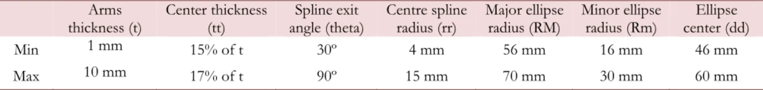
This geometry is defined by nine variables. Two of them where considered constant, the specimen arm length with a value of 200 mm and the specimen arm width with a value of 30 mm for finite element modeling purposes. These dimensions have no influence on the final results. The specimen arm width is also a possible variable for future optimization problems, as it will influence the applied load in order to achieve a desirable stress level. Tab. 1 shows five of the other variables which were used in the optimization problem. The center thickness (tt) is a value of the arms thickness (t) (material base) and ratios of 15% and 17% were considered, while the spline exit angle (theta) is a very important variable ensuring a smooth geometrical transition to avoid stress concentration in the critical region. The center spline radius (rr) defines the area where the specimen thickness is reduced, using the above referenced revolved spline, that has a tangency

T

(3)

120

of 0º at the center. The elliptical fillet is centered between the specimen arms and is defined by three variables, the major ellipse radius (RM), the minor ellipse radius (Rm) and the ellipse center (dd).

Figure 1: Specimen geometry, dimensions in mm.

Arms thickness (t) Center thickness (tt) Spline exit angle (theta) Centre spline radius (rr) Major ellipse radius (RM) Minor ellipse radius (Rm) Ellipse center (dd) Min 1 mm 15% of t 30º 4 mm 56 mm 16 mm 46 mm Max 10 mm 17% of t 90º 15 mm 70 mm 30 mm 60 mm

Table 1: Design variables used in the specimen design geometry optimization.

Finally the specimen arms thickness (t) is also a variable and one of the most important. This was the base variable for all the optimizations performed in the present work. In order to achieve on the main goals, the arms thickness was chosen using the Renard Series of Preferred Numbers [16], which is used as a base for material standard presentation by sheet manufactures. Therefore the present results may be directly used by the end user. Tab. 2 shows the used arms thickness on the present paper, in order to optimize the geometry shown in Fig. 1.

R10″ 1 2 3 4 5 6 7 8 9 10 11

Arms thickness (t) [mm] 1.00 1.20 1.50 2.00 2.50 3.00 4.00 5.00 6.00 8.00 10.00

Center thickness (tt) [mm] 0.17 0.20 0.25 0.33 0.42 0.50 0.67 0.83 1.00 1.20 1.50

Table 2: Design variables used in the specimen design geometry optimization.

The series chosen is the R10″, which is rounded, between 1 mm and 10 mm of the arms thickness. I order to simplify the optimization problem to five active variables, the problem was solved individually for each arm thickness and center thickness as provided in Tab. 2. This variable can, and will also be explored in future works, but on the present paper was kept constant with a value of 17% of the arms thickness, except for the higher values of 8 and 10 mm, where it was kept constant on 15%, because the optimization convergence was not able to be met with the previous value. These ratios were considered from previous optimization results, where the arms thickness was an active variable, [11].

(4)

121

MULTI-OBJECTIVE OPTIMIZATION

constrained nonlinear multi-objective optimization problem (MOO) can be mathematically formulated as, [17]: Find n design variables:



1, ...,2



T n x  x x x (1) which minimizes:

 



1

   

2

 



. .min , ,..., T k s t xF x  f x f x f x (2)

involving k objective functions : n

 

, 1,...,

j

f      j  k to minimize.

Recall that to maximize fj is equivalent to minimize -fj.





n

     represents the feasible region.

Any or all functions fj, j=1,…,k can hold a nonlinear nature. In general, since in MOO there are often conflicting

objectives for each objective function, the concept of Pareto dominance is used to characterize global and local optimality, [17]. A feasible solution of x is called a Pareto optimal if there exists no other feasible solution y such that fi(y)≤fi(x) for all

i={1,2,…,k} with fj(y) < fj(x) for at least one j, j ∈ {1,2,…,k}.

The Direct MultiSearch (DMS) algorithm [17] is a derivative-free method for multiobjective optimization problems. This algorithm does not aggregate or scalarize any components of the objective function and it is inspired by the search-poll paradigm of direct-search methods of directional type from single to multiobjective optimization. Through the use of the concept of Pareto dominance, this algorithm generates and maintains a list of feasible nondominated points from which it iterates and chooses new poll centers. The DMS algorithm tries to capture the whole Pareto dominance front from the polling procedure and at each iteration, if improvement is found, the new feasible evaluated points are added to the list (approximating the Pareto front) and the dominated ones are removed. Successful iterations then correspond to changes in the approximation of the Pareto front meaning that a new feasible nondominated point was found, otherwise, the iteration is declared as unsuccessful. The search step is optional and set as to best fit to the optimization problem characteristics in order to improve the numerical performance. In Direct MultiSearch, constraints are handled using an extreme barrier function:

 

_

 

_

,..., F x if x F x otherwise      _ _  (4)

Which means that if a point is infeasible (not belonging to the predetermined feasible points universe or compromised by the problem constraints), the components of the objective function F are not evaluated and the values of F are set to +∞. This approach allows us to deal with black-box type constraints where only a yes/no answer is returned.

Optimization procedure

The optimization procedure uses three different programs. Initially MATLAB creates an input file with the initial design variables values. These variables, as referred in Tab. 1, are the minor ellipse radius (Rm), the major ellipse radius (RM), the ellipse center (dd), the center spline radius (rr) and the spline exit angle (theta), whose limits (introduced as restrictions) are given in Tab. 1. Using a PYTHON script the resulting geometry is created by Finite Element Method (FEM) code ABAQUS, as well as all the loads and boundary condition are applied to the model. The chosen material is an aluminium alloy with Young modus of 69 GPa and Poisson ratio of 0.3. Once solved all the necessary stresses and strains are saved in to individual files, which are read by MATLAB in order to validate the solution and to calculate the two objective functions, using Eq. (5) and (6):

F1(x) = - σMaximum Von Mises Stress Level on Specimen Center (5)

F2(x) = max(δσCenter Stress/σCenter Stress) (6)

The first objective function is the negative value of the maximum stress level on the specimen center, and the second objective function is the maximum stress level difference within a 1m radius of the specimen center. Using the DMS

(5)

122

algorithm described above a new set of design variables are calculated, and by repeating this procedure the Pareto Front will be generated.

Load cases and Boundary Conditions

The optimization process used a simplified version of the cruciform specimen for FEM calculations. Due to symmetry, 1/8 of the geometry was modeled and symmetry boundary conditions were applied to all three symmetry planes.

32315 tridimensional linear elements were used, with a total of 40548 nodes per simulation. Also two different load cases were studied, the first load case is an in-phase (δ=0º) loading, with a 1 kN load applied in both directions. The second load case is an out-of-phase (δ=180º) loading, with a 1 kN load applied on one direction and a – 1 kN load applied to the second direction.

For both load cases the validation conditions where the same. The difference between the maximum stress level on the specimen center and the arms must be higher than 20%, while the stress differences in both directions within a 1mm radius of the specimen center must be lower than 2%. Therefore one can guaranty that the maximum stress level occurs on the specimen center, and is uniform enough in order for the geometry to be appropriated for fatigue crack initiation.

SPECIMEN OPTIMIZATION RESULTS

fter running the optimization procedure for every arms thickness on Tab. 2, it was possible to obtain several optimized specimen geometry, as exemplified on Tab. 3. Each configuration of variables where chosen from each of the Pareto Fronts obtained for the Renard series of Tab. 2. They do not represent the global optimum solution for the maximum stress level, or stress uniformity level, they were chosen within the Pareto Front in order to produce a smooth evolution for every variable, as the arms thickness is changed. Therefore it will possible to attain a relationship between those variables and the arms thickness.

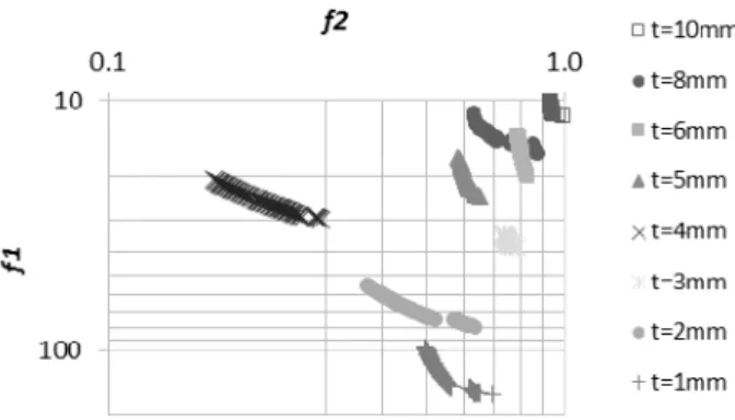
Each configuration on Tab. 3, represents a point on the Pareto Front (Fig. 2) for the corresponding value of arms thickness, any point of the Pareto Front could have been chosen, as they all are mathematically equal. But the main goal of this paper is to establish a relationship between every specimen geometry variable and the arms thickness, therefore Tab. 3 represents the best configurations possible to achieve this goal.

t, mm

(fixed) RM, mm Rm, mm Theta, º rr, mm dd, mm tt, mm (fixed) Maximum Stress, MPa/kN Difference, % Stress

1.0 61.7 22.5 71 5.9 51.3 0.166 146 0.657 1.2 62.2 21.9 68 5.0 52.0 0.200 109 0.931 1.5 62.7 22.0 64 5.0 52.4 0.250 87 0.859 2.0 63.9 22.3 36 5.8 52.4 0.334 76 0.587 2.5 61.6 22.3 60 5.5 51.7 0.416 53 0.784 3.0 60.1 22.3 66 5.2 51.7 0.500 37 0.753 4.0 58.7 25.8 38 9.1 51.3 0.666 29 0.284 5.0 56.0 25.8 45 9.6 49.9 0.834 22 0.616 6.0 56.7 25.8 43 9.8 50.1 1.000 19 0.825 8.0 63.4 28.6 72 9.8 55.1 1.200 15 0.715 10.0 65.1 28.6 70 9.9 57.6 1.500 10 0.932

Table 3: Optimal specimen geometry for each Renard series value of arms thickness.

(6)

123

Arms thickness influence

The arms thickness influence changes the optimal specimen geometry in different ways when one analyses the different variables used in this optimization. In Fig. 3 it is possible to assess the influence of the arms thickness on the form and position of the elliptical fillet used between the specimen arms. One can see that for arm thickness values less than 2 mm, both the major and minor ellipse radius, RM and Rm, increase with the arm thickness. Then both these values decrease, between 2 and 6 mm of arm thickness, before they will increase again. In a different way the position of the center of the elliptical fillet position (dd) is directly proportional to the arms thickness.

The variables used to define the revolved spline for the specimen center generation are also influenced by the arms thickness. The center thickness was considered constant in every optimization, therefore the centre spline radius and spline exit angle, rr and theta, variation can be found in Fig. 4 and Fig. 5. Both these variables are related, as it will be discussed next, but their variation with the arms thickness is clear. The center spline radius is almost constant for thickness values less than 3 mm, before it starts to increase very rapidly between thicknesses of 4, 5 and 6 mm. Then it is almost constant again for higher thickness values. The spline exit angle clearly decreases with the thickness, for values less than 4 mm, before it starts to increase again. Some optimal configurations do not represent this behavior, but some of these exceptions can be justified by the spline exit angle and centre spline radius influence discussed next. Lines plotted in Fig. 3 to 5 represents the polynomial interpolation to the points.

Spline exit angle and centre spline radius influence

The specimen geometry contain on its center a revolved spline defined by three variables. Two of them are very important for the maximum stress level and stress uniformity level. Considering all the points on the Pareto Fronts one can see that decreasing the spline exit angle, the maximum stress level on the specimen center increases, while the stress uniformity level decreases. In order to justify this effect, one must consider the spline profile. As the spline exit angle decreases, the slope around the specimen center becomes steeper, increasing the stress level but decreasing the stress uniformity.

The center spline radius has the same effect. Increasing the center spline radius, increases the size of the area where the thickness in reduce, therefore increasing the stress uniformity level while decreasing the maximum stress level. Again the spline profile, is responsible for this effect.

Figure 2: Pareto Fronts for several arms thickness Figure 3: Arms thickness influence on the elliptical fillet.

(7)

124

Combining both variables allows the optimization process to generate points where both the maximum stress level and the stress uniformity level are optimal. Combining these points with the other variables, it is possible to obtain the Pareto Fronts provided on Fig. 2. Analyzing the Pareto Fronts it is possible to report that sometimes the optimization algorithm achieved better results by decreasing the value of the spline exit angle while increasing the value of the center spline radius, this happened for the arms thickness of 2 mm. Unfortunately this behavior leads to a difficult correlation between the center spline radius or the spline exit angle variables and the arms thickness, as seen on Fig. 4 and 5.

Center thickness influence

The influence of the center thickness was studied in the preparation work for this paper. The center thickness is the most important variable on the specimen center maximum stress optimization. This variable dominates all the others and using it on the optimization process, means this variable will always assume the lower bound value. Therefore decreasing the center thickness, increases the maximum stress level, while the stress uniformity decreases. Considering the domination effect the center thickness was considered fixed on the present results. The authors decide to start with a relationship of 17% between the center thickness and the arms thickness, based on past works by Cláudio et al. [11]. Nevertheless as the arms thickness increases with the Renard series number, for values of 8 and 10 mm, it was impossible to achieve convergence of the optimization process using a 17% ratio. The solution used was to decrease the center thickness, and a 15% ratio was used, as seen on Tab. 3.

Future work planed by the authors will include the use of different ratios between the center and arms thickness, in order to establish the relationship between both these variables and the optimal specimen geometry.

Stress distribution on the specimen center

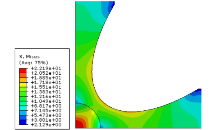
The conditions for solution acceptance in the optimization process, included the center maximum stress to be 20% higher than the arms maximum stress (based on several experimental tests experience), and the stress differences on the specimen center to be less than 2% in 1 mm radius (accepted reasonable limit for the authors). Considering that the stress uniformity level was an optimization objective, it was expected to achieve even lower center stress differences. Fig. 6 shows the evolution of the center stress differences with the Renard series thickness values (also according to Tab. 3), one can see the maximum value is 0.93%. Fig. 7 shows the Von Mises stress distribution around the center of a specimen with 5 mm of arms thickness for the first load case (proportional). It is possible to see how the stress level is almost constant on the specimen center, while the arms stress is always at an inferior level. By changing the loading conditions, one can see on Fig. 8 how the stress distribution remains almost constant on the specimen center, even with the presence of non-proportional load case with a phase shift of 180º.

Finally Fig. 9 shows the relationship between the arms thickness and the optimal maximum stress level on the specimen center. As expected the stress level decreases as the arms thickness increases. Fig. 9 shows the maximum stress levels for the first load case, it can be shown that on the second load case, the Von Mises stress level is 3.4 time higher, while the normal stress levels are 2 times higher.

Final specimen optimal geometry

Following the present results it is possible to recommend the use of an optimal geometry as a function of the material arms thickness, using Eq. (7) to (13), which are plotted in Fig. 3 to 5:

RM(t) = -0.0379t4_{+ 0.8223t}3_{- 5.5749t}2₊_12.555t₊_53.84₍₇₎ Rm(t) = -0.0236t3_{+ 0.3501t}2_{- 0.5036t + 22.185} ₍₈₎ dd(t) = -0.021t4_{+ 0.4668t}3_{- 3.248t}2_{+ 7.9452t + 46.224} ₍₉₎ rr(t) = -1.2979t3_{+ 8.1814t}2_{- 16.157t + 15.071} _{for: 1 ≤ t ≤ 3 mm} ₍₁₀₎ rr(t) = 0.0171t3_{- 0.3968t}2_{+ 3.0199t + 2.2763} _{for: 4 ≤ t ≤ 10 mm} ₍₁₁₎ theta(t) = 2.0201t3_{- 3.4534t}2_{- 14.954t + 87.4} _{for: 1 ≤ t ≤ 3 mm} ₍₁₂₎ theta(t) = -0.7621t3_{+ 15.484t}2_{- 92.774t + 211.78} _{for: 4 ≤ t ≤ 10 mm} ₍₁₃₎

These equation are valid for 1≤ t ≤ 10 mm and considering that tt is equal to 0.17t, for t<8 mm and tt equal to 0.15t if t≥8 mm. Also these equations are not valid for t=2mm, as the behavior on this point is significantly different.

Future validation and extra work will allow to include on the previous equations the influence of the center thickness (tt), and therefore construct a standard cruciform specimen geometry for biaxial fatigue in-plane testing.

(8)

125

Figure 6: Center stress differences. Figure 7: Stress distribution in the optimized geometry, t=5mm,

Load Case 1.

Figure 8: Stress distribution in the optimized geometry,

t=5mm, Load Case 2.

Figure 9: Maximum center stress, Load Case 1.

CONCLUSIONS

he Direct Multi-Search model was able to produce several Pareto Fronts for a very complicated Finite Element problem, which included two objective function and five active design variables. Each Pareto Front was obtained for each arms thickness, based on the Renard series of preferred numbers, and therefore the specimen designer can obtain the optimal geometry as a function of the desired material thickness. Within the Pareto Front all the specimen geometries configurations are mathematically equal, therefore the ones chosen in this paper represent the best possible correlation between the design variables and the arms thickness. It was possible to achieve a correlation between the arms thickness and the specimen elliptical fillet variable. On the other hand the relationship between the center spline radius or the spline exit angle and the arms thickness still need to be worked on. Both these variables have the same effect on the maximum stress level and stress uniformity level on the specimen center. Decreasing their value leads to an increase on the maximum stress level and a decrease on the stress uniformity level. Therefore different combinations lead to similar results. Decreasing the specimen center reduced thickness value leads to higher stress levels, but is was found that this is a dominating variable. Therefore the center thickness was assumed constant, sa ratio of the arms thickness, in the optimization process. Future work will require to achieve a correlation between this variable and the other specimen design variables. Two different loading conditions were studied, and it is possible to report that the second load case produces higher stress levels on the specimen center. .As expected increasing arms thickness decreases the maximum stress level on the specimen.

REFERENCES

[1] Shanyavskiy, A., Fatigue cracking simulation based on crack closure effects in Al-based sheet materials subjected to biaxial cyclic loads, Eng. Fract. Mech., 78 (8) (2011) 1516–1528.

(9)

126

[2] Cláudio, R. A., Freitas, M., Reis, L., Li, B., Guelho, I., Multiaxial Fatigue Behaviour of 1050 H14 Aluminium Alloy by a Biaxial Cruciform Specimen Testing Method, In: 10th Int. Conf. Multiaxial Fatigue Fract., (2013).

[3] Cláudio, R., Freitas, A. M., Reis, L., Li, B., Guelho, I., Antunes, V., Maia, J., In-plane biaxial fatigue testing machine powered by linear iron core motors, Sixth Symp. Appl. Autom. Technol. Fatigue Fract. Test. Anal., ASTM STP 1571 (2013).

[4] Hanabusa, Y., Takizawa, H., Kuwabara, T., Numerical verification of a biaxial tensile test method using a cruciform specimen, J. Mater. Process. Technol., 213(6) (2013) 961–970.

[5] Müller W., Pöhlandt, K., New experiments for determining yield loci of sheet metal, J. Mater. Process. Technol., 60(I 996) (1996) 643–648.

[6] Bruschi, S., Altan, T., Banabic, D., Bariani, P. F., Brosius, A., Cao, J., Ghiotti, A., Khraisheh, M., Merklein, M., Tekkaya, A. E., Testing and modelling of material behaviour and formability in sheet metal forming, CIRP Ann. - Manuf. Technol. (2014).

[7] Leotoing, L., Guines, D., Zidane, I., Ragneau, E., Cruciform shape benefits for experimental and numerical evaluation of sheet metal formability, J. Mater. Process. Technol., 213(6) (2013) 856–863.

[8] Yu, Y., Wan, M., Wu, X.-D., Zhou, X.-B., Design of a cruciform biaxial tensile specimen for limit strain analysis by FEM, J. Mater. Process. Technol., 123(1) (2002) 67–70.

[9] Smits, A., Van Hemelrijck, D., Philippidis, T. P., Cardon, A., Design of a cruciform specimen for biaxial testing of fibre reinforced composite laminates, Compos. Sci. Technol., 66(7–8) (2006) 964–975.

[10] Makris, A., Vandenbergh, T., Ramault, C., Van Hemelrijck, D., Lamkanfi, E., Van Paepegem, W., Shape optimisation of a biaxially loaded cruciform specimen, Polym. Test., 29(2) (2010) 216–223.

[11] Guelho, I., Reis, L., Freitas, M., Li, B., Madeira, J. F. A., Cláudio, R. A., Optimization of Cruciform Specimen for a Low Capacity Biaxial Testing Machine, In: 10th Int. Conf. Multiaxial Fatigue Fract., (2013).

[12] Poncelet, M., Barbier, G., Raka, B., Courtin, S., Desmorat, R., Le-Roux, J. C., Vincent, L., Biaxial High Cycle Fatigue of a type 304L stainless steel: Cyclic strains and crack initiation detection by digital image correlation, Eur. J. Mech. - A/Solids, 29(5) (2010) 810–825.

[13] Ackermann, S., Kulawinski, D., Henkel, S., Biermann, H., Biaxial in-phase and out-of-phase cyclic deformation and fatigue behavior of an austenitic TRIP steel, Int. J. Fatigue, 67 (2014) 123–133.

[14] Lamkanfi, E., Van Paepegem, W., Degrieck, J., Ramault, C., Makris, A., Van Hemelrijck, D., Strain distribution in cruciform specimens subjected to biaxial loading conditions. Part 1: Two-dimensional versus three-dimensional finite element model, Polym. Test., 29(1) (2010) 7–13.

[15] Makinde, A., Thibodeau, L., Neale, K., Development of an apparatus for biaxial testing using cruciform specimens, Exp. Mech., 32(2) (1992) 138–144.

[16] O. for Standardization, ISO 3, Preferred numbers — Series of preferred numbers, (1973).

[17] Custódio, A.L., Madeira, J.F.A., Vaz, A.I.F., Vicente, L.N., Direct multisearch for multiobjective optimization, J. Optim., (2011) 1–33.