WORKING PAPER SERIES
CEEAplA WP No. 05/2009
Welfare Impacts of Road Construction Using a
Public-Private Partnership: a CGE Analysis of
a Project
Ali Bayar Mário Fortuna Sameer Rege March 2009
Welfare Impacts of Road Construction Using a
Public-Private Partnership: a CGE Analysis of a Project
Ali Bayar
Universite Libre de Bruxelles
Departement D’Economie Appliquee
EcoMod
Mário Fortuna
Universidade dos Açores (DEG)
e CEEAplA
Sameer Rege
Universidade dos Açores (DEG)
e CEEAplA
Working Paper n.º 05/2009
Março de 2009
CEEAplA Working Paper n.º 05/2009 Março de 2009
RESUMO/ABSTRACT
Welfare Impacts of Road Construction Using a Public-Private Partnership: a CGE Analysis of a Project
The Azorean Government embarked on a public-private partnership to build a road on the island of São Miguel, to circumvent the budget restriction imposed by the central government. We build a sequentially dynamic general equilibrium model with 45 sectors to measure the welfare changes arising from the project. The initial investment is amortised over a period and the payments are simulated through an increase in income taxes, reduction in transfer payments or calculating the fall in transport margins. We find that under any type of repayment scheme the welfare benefits do not justify the road construction thus making it a poor investment decision.
Ali Bayar
Universite Libre de Bruxelles
Departement D’Economie Appliquee Avenue Paul Heger 2
B-1000 Bruxelles Mário Fortuna
Departamento de Economia e Gestão Universidade dos Açores
Rua da Mãe de Deus, 58 9501-801 Ponta Delgada Sameer Rege
Departamento de Economia e Gestão Universidade dos Açores
Rua da Mãe de Deus, 58 9501-801 Ponta Delgada
Welfare Impacts of Road Construction Using a Public -Private Partnership: A CGE Analysis of a Project
Ali Bayar, Université Libré de Brussels, Brussels, Belgium,
Mário Fortuna** CEEAplA and Departmento de Economia e Gestão, Universidade dos Açores, Portugal,
Sameer Rege* CEEAplA and Departmento de Economia e Gestão, Universidade dos Açores, Portugal,
Abstract
The Azorean Government embarked on a public-private partnership to build a road on the island of São Miguel, to circumvent the budget restriction imposed by the central government. We build a sequentially dynamic general equilibrium model with 45 sectors to measure the welfare changes arising from the project. The initial investment is amortised over a period and the payments are simulated through an increase in income taxes, reduction in transfer payments or calculating the fall in transport margins. We find that under any type of repayment scheme the welfare benefits do not justify the road construction thus making it a poor investment decision.
** Correspondent author *
1.0 Introduction
In an attempt to circumvent budget restrictions, some governments have resorted to public/private partnerships in order to construct infrastructure. This approach to create amenities infeasible within the government budget has, in the past, been associated with projects that charge user fees like tolls to pay for services, such as major roads, bridges and the like. An innovation of this approach has been to levy no fees to user and have the government assume the cost of what will be a virtual toll. This approach has been extensively used in recent years in Portugal and has also been adopted on the island of São Miguel, part of the Portuguese archipelago of the Açores.
Bound by the stability and growth pact associated with the single currency of the European Union, the Portuguese government has resorted to operations off the national budget.
The Azorean government has embarked on a similar programme to solicit initial investment from the private sector to build a road and amortise the payment over a span of twenty-five years, after completion to be paid through taxes collected. NPV and IRR methods do not account for the change in the behaviour of individuals due to change in the taxes levied for undertaking such an enterprise. The criteria for measuring the benefit from such a project should be the impact on welfare as accounted via the utility functions. Individuals know that the road is toll free but will be paid via taxes in the future and knowing this will modify their behaviour accordingly and thus impact capital accumulation and growth.
To analyse the welfare impacts of this project, we use a sequentially dynamic general equilibrium model built with the latest data on the Azorean economy at the 45 sector level. The main issues are: What economic benefits are derived from the
improved road? What is the impact of increasing taxes to pay for the road? What are the welfare impacts of reducing transfers to compensate the extra expenditure? The following scenarios are considered: a reduction in the transfers to the households equal to the amortisation and, finally; a reduction in the transport margins that should improve the efficiency of the economy.
In what follows, section 2.0 describes, in detail, the set-up of the project and its implications on the regional economy and on the public finances. Section 3.0 spells out the major features of the CGE model that are used to run the simulations for each scenario considered. Section 4.0 analyses the scenarios considered and the results obtained. Section 5.0 reviews the main conclusions and advances some suggestions for future work.
CGE models have been used extensively for policy analysis and are a standard tool of empirical analysis. They are useful to analyze the aggregate welfare and distributional impacts of policies whose effects may be transmitted through multiple markets, or contain plethora of different tax, subsidy, quota or transfer instruments. From the perspective of the individual decisions can be either myopic or with perfect foresight. In the former case, the individual is faced with a two-period maximization problem and the saving decision is based on this choice. With perfect foresight, the individual solves a dynamic optimization problem with consumption being the control variable that determines the level of savings and eventually the capital stock and growth. Heer and Maussner (2005) cover the theory of dynamic general equilibrium along with overlapping-generations models. From our perspective the decision to construct or not construct a road is primarily a government decision and since it will be a public good devoid of marginal cost pricing in absence of a toll, we have embarked on
a detailed sector specification of the economy rather than an aggregate dynamic model analysing the present value of welfare from the road construction.
2.0 A Public/Private Partnership for the Construction of a Major Road
The archipelago of the Açores, comprises 9 islands of which São Miguel is the largest, accounting for 60% of the GDP and 50% of the population. In 2007, the regional government of the Açores contracted the construction/repair of a major road in São Miguel. The project affects about 50% of the stock of major roads in the island and will impact on about 80% of the traffic.
The project is as follows: on a first, immediate phase, the government gives concession of existing roads to a private company that will assume its upkeep. The government receives a payment of €17,624,608 in the first year and €846,972 during the second, from the company. Simultaneously, for a period of five years, the company will construct/repair the predetermined road sections costing €750000 each year for four years. As of the sixth year, the government will start payment of the accumulated debt on a schedule that is expected to imply outlays of around €325 million.
Debt, comprising the initial payments by the private company, construction during five years, maintenance costs and interest on outstanding debt, accumulates during the first five years to determine the total that will be reimbursed as of the sixth year. Given the payment schedule, it is estimated that the base value of the project, consisting of new construction, will be €100 million, spread evenly (€ 20 million) along each of the five years.
Until the end of the fifth year there are no outlays by the government. In fact, government expenditures are potentially increased as there advances from the private concession on the first two years. Debt accumulates until it reaches an estimated 168 million euros by the end of the fifth year. Repayment starts on the sixth year at an annual value of around 12.5 million euros, for twenty five years.
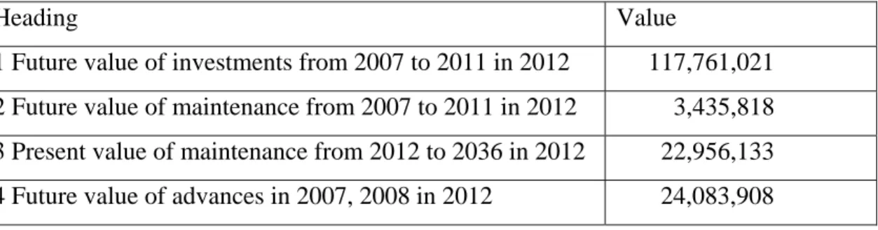
Table 1 summarizes the values at stake, assuming an average interest rate of 5.5%. Table 1: Present Value of Construction Liabilities in time 5 or year 2012
Heading Value 1 Future value of investments from 2007 to 2011 in 2012 117,761,021
2 Future value of maintenance from 2007 to 2011 in 2012 3,435,818 3 Present value of maintenance from 2012 to 2036 in 2012 22,956,133 4 Future value of advances in 2007, 2008 in 2012 24,083,908
5 Total Liabilities in 2012 (5=1+2+3+4) 168,236,880
The accumulated obligations, at the end of the fifth year, amount to about €168,236,880, associated to new construction of about 100 million euros. The reimbursement schedule is based on annual repayment that implies an annual outlay by the government of €12,541,951.
The main question is can this project be justified and what are the metrics to decide in favour or against this project? Standard economic literature emphasises the change in welfare arising from a change in utility would be a right metric to assess the potential gain/loss from this project.
The gains will certainly come from the initial additional expenditures that, we will assume, trickles through the economy according to its current structure. Once the roads are completed, one should also expect that travel costs will be lower. In our model this will imply that transport margins are lower.
The costs will be associated to the reimbursement of the debt that is accumulated. Since it is assumed that the government will not be able to increase its debt stock, total payment will have to be made out of additional taxes from economic growth prompted from better and more economical roads, additional taxes on the citizens, or less transfers to the citizens, from the government.
The scenarios considered are, therefore, based on:
1. the implicit reduction in transport margins on the land transport sector; 2. imposition of an additional income tax on the households;
3. reduction in the amount of transfers of the households.
3.0 The Model
The Azorean economy, represented by a sequentially dynamic multi-sector computable general equilibrium model (CGE), incorporates the behaviour of six economic agents: firms, households, regional government, Mainland government, European Commission and the Rest of the World (ROW). For detailed equations and model specification refer Fortuna et. al (2009)
The goods-producing sectors, consisting of both public and private enterprises, are disaggregated into 45 branches of activity. Households are divided into six income groups q1 (poorest) to q6 (richest), to analyze the distributional effects of various policy
measures. Special attention is paid to the economic links between the regional government, the Mainland government and the European Commission. With regard to the rest of the world the economy is treated as a small open economy with no influence on (given) world market prices. Trade relations are differentiated according to four main trade partners: Mainland, EU, US and the rest of the world. The model has been solved by using the general algebraic modelling system GAMS (Rosenthal, 2006).
The model is sequentially dynamic, hence individuals are myopic and factor only the current period return to capital to decide on savings. The return to capital in turn responds to the demand and supply for each good as the capital is sector specific. Thus any policy changes affect return to capital and hence determine investment decisions and new capital into each sector. The rest of the model behaviour is again supply– demand driven with price adjustment playing the major role. Domestic markets adjust to domestic demand-supply. The domestic supply is a function of foreign demand and exchange rates. The labour demand is endogenous and unemployment responds to wages.
3.1.Firms
All firms operate in an environment of perfect competition implying price equals marginal cost with constant returns to scale. The level of production for each branch of activity is determined from a nested production structure (see Figure 1). A Leontief production function determines the fixed share of inputs and value added in output. The maximization of value added or minimization of factor costs (labour and capital) determine the demand for labour and capital in each sector. The functional form used is a CES. The wage differential across industries is modelled through a premium or discount to the average wage prevalent in all industries. The social sector contributions and tax rates on private capital are specified according to the government regulations. Capital is industry specific, introducing rigidities in the capital market. The inter-sectoral wage differential is a parameter derived as the ratio between the wage by branch and the national average wage (Dervis, De Melo and Robinson, 1982). Holding the inter-sectoral wage differentials constant in counterfactual policy simulations introduces rigidities in the labour market.
Figure1. The nested Leontief and CES production technology for the domestic production by branch of activity
Each activity produces primary and secondary products and services which are then allocated to domestic and export markets based on the prices in those markets so as to maximise the value added. The output of each product or service is a fixed coefficient Leontief function of each activity of a branch. Treated at an aggregate level, firms’ savings are given by a share of the net operating surplus.
3.2. Households
Households are split into six income groups (q1-q6), the first group being the poorest one. The representative household in each income group receives a part of the capital income (net operating surplus), a part of the labour income, unemployment benefits from the Mainland government and other net transfers from the regional and Mainland governments. The representative household in each income group pays income taxes and saves a share of the net income. Each household saves according to a Marginal Propensity to Save that responds to the after-tax average return to capital. Any changes that affect the return to capital impact the savings and thus the growth. The difference between the income and savings is the disposable income which is allocated between different goods and services according to a Stone-Geary utility function.
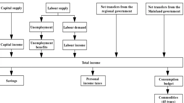
In the allocation process, the consumer first decides on the minimum (subsistence) level of consumption of commodity c. Then, the marginal income is allocated between different types of commodities according to the marginal budget shares. A schematic representation of households’ decisions, by income group, is given in Figure 2.
Domestic production by branch
Value-added Intermediates
Capital supply Labour supply
Une mployme nt Labour de mand
Une mployme nt
be ne fits Labour income Capital income Total income Savings Pe rsonal income taxe s Consumption budge t Ne t transfers from the
re gional gove rnment
Net transfe rs from the Mainland gove rnme nt
Commoditie s (45 type s)
Figure 2. Decision structure of the representative household by income group
Household welfare gains/losses are valued using the equivalent variation in income, which is based on the concept of a money metric indirect utility function (Varian, 1992) corresponding to the Linear Expenditures System (LES) in the counter-factual (policy scenario) equilibrium.
Equivalent variation measures the income needed to make the household as well off as she is in the new counter-factual equilibrium (policy scenario) evaluated at benchmark prices. Thus, the equivalent variation is positive for welfare gains from the policy scenario and negative for losses.
3.3. Regional government
Regional government collects all the taxes, such as: taxes on income and wealth and taxes on products and on production and receives transfers from the Mainland government, EU funds and transfers from the external sector
Taxes on products are differentiated in the model according to the category of consumption on which they apply: intermediate consumption, private consumption, and gross capital formation.
The total transfers received by the regional government are given by transfers from the Mainland government, transfers from EU as direct subsidies on production and other transfers from EU, transfers from US and transfers from the rest of the world, where the transfers are expressed in domestic currency using the exchange rate with respect to Mainland, the exchange rate with respect to EU, the exchange rate with respect to US and the exchange rate with respect to the rest of the world.
Regional government expenditures comprise the public current consumption, total transfers by the government and subsidies on products and on production
The optimal allocation of the public current consumption between different types of goods and services is given by the maximization of a Cobb-Douglas function subject to the budget constraint
Total transfers by the regional government include transfers to the households translated into nominal terms by using the Laspeyres consumer price index.
The EU funds as direct subsidies on production are transferred to the regional government budget which allocates them between different branches of activity. The difference between the regional government revenues and the government expenditures yields the government savings.
Mainland government collects all the social security contributions, provides unemployment benefits and makes transfers to the households and to the regional government.
Social security contributions are derived by applying the social contributions rate to gross wages. Unemployment benefits received by each household income group are determined by the combination of the replacement rate, the national average wage, the total number of unemployed, and the share of unemployed subject to unemployment benefits in each household income group.
European Commission provides EU funds as direct subsidies to the production sectors and other EU funds to the regional government.
3.4. Foreign trade
The specification of the foreign trade is based on the small-country assumption, which means that the country is a price taker in both its import and its export markets. Four different trade partners are distinguished in the model: Mainland, EU, US and the rest of the world.
On the import side, imperfect substitution is assumed between domestically produced and imported goods, according to the Armington function. Thus, domestic consumers use composite goods of imported and domestically produced goods, according to a CES function. In a similar fashion, the differentiation between the exported goods by the domestic producers to Mainland, EU, US and to ROW and the domestic goods supplied on the domestic market is captured through a constant elasticity of transformation (CET) function.
By maximizing the revenue, subject to the CET function, we derive the supply of exports by the domestic producers to Mainland, to EU, to US and to ROW and the supply by the domestic producers to the domestic market.
In addition, export demand functions are introduced in the model such that the export demand for domestically produced goods by the external sector, depends on the benchmark level of the export demand by the foreign sector, the relative price change and the price elasticity of export demand. The market clearing equations for exports determine the domestic price of exports received by the domestic producers.
Balance of payments, expressed in foreign currency, takes into account all the trade and capital flows and is differentiated according to each trade partner.
3.5. Investment demand
Total savings used to buy investment goods are given by a sum of, the households savings by income group, firms savings, gives the regional government savings, expressed in nominal terms using the GDP deflator, and is the depreciation related to the private and public capital stock. The balance of the current accounts corresponding to Mainland, EU, US and ROW are expressed in domestic currency using the exchange rates with respect to Mainland, to EU, to US and to the rest of the world.
3.6. Price equations
A common assumption for CGE models, which has also been adopted here, is that the economy is initially in equilibrium with the quantities normalized in such a way that prices of commodities equal unity. Due to the homogeneity of degree zero in prices, the model only determines the relative prices. Therefore, a particular price is selected to provide the numeraire against which all relative prices in the model will be measured. We choose the GDP deflator as the numeraire.
Different prices are defined for all the branches, exports and imports. As already explained, trade and transport margins are paid on all categories of demand in AzorMod except the government consumption (on intermediate consumption, on private consumption and on investment goods).
The domestic price of imports is determined by the price of imports expressed in foreign currency and the exchange rate.
3.7.Labour market
The labour supply minus the labour demand equals unemployment. The responsiveness of real wage to the labour market conditions is modelled by a wage curve as in Sanz-de-Galdeano and Turunen (2006). The labour supply responds to the ratio of the price index in
the base to the price index in the counterfactual according to the elasticity of labour supply. The national employment is defined as labour supply minus unemployment. The national average wage including social security contributions is determined via the national average wage and the wage premium is sector s and the social contributions rate in sector s.
3.8.Market clearing equations
The equilibrium in the product, capital and labour markets requires that demand equals supply at prevailing prices (taking into account unemployment for the labour market). Labour market clearing equation has already been presented above. Capital stock is sector specific, such that the equality between capital demand and supply determines the return to capital by branch of activity.
Separate market clearing equations are distinguished in the model for each commodity c. For the trade and transport services, the sum of demand for intermediate consumption of commodity, the private demand for commodity, the public demand for commodity, the demand for investment goods, the demand for inventories and the demand for trade and transport services which are invoiced separately (trade and transport margins) should be equal with the total supply of commodity from imports and domestic production.
The demand for trade and transport services invoiced separately as per Löfgren, Harris and Robinson, (2002), is further derived as the sum of demand for trade and transport services on private consumption, of demand for trade and transport services on investment goods and of demand for trade and transport services on intermediate consumption. The demand for inventories for each commodity c is defined as a fixed share of domestic sales.
3.9.Incorporation of dynamics
AzorMod has a recursive dynamic structure composed of a sequence of several temporary equilibria. The first equilibrium in the sequence is given by the benchmark year. In each time period, the model is solved for an equilibrium given the exogenous conditions assumed for that particular period. The equilibria are connected to each other through capital accumulation. Thus, the endogenous determination of investment behaviour is essential for the dynamic part of the model. Investment and capital accumulation in year t depend on expected rates of return for year t+1, which are determined by actual returns on capital in year t.
The normal rate of return to capital in branch s is specified as an inverse logistic function of the proportionate growth in sector’s s capital stock Dixon and Rimmer, (2002).
index. The capital stock in industry s in the next period (year t+1) is given as a function of the current capital stock (in year t) and the investments by the branch s in year t. The model is solved dynamically with annual steps.
3.10. Closure rules
The closure rules refer to the manner in which demand and supply of commodities, the macroeconomic identities and the factor markets are equilibrated ex-post. Due to the complexity of the model, a combination of closure rules is needed. The particular set of closure rules should also be consistent, to the largest extent possible, with the institutional structure of the economy and with the purpose of the model.
In mathematical terms, the model should consist of an equal number of independent equations and endogenous variables. The closure rules reflect the choice of the model builder of which variables are exogenous and which variables are endogenous, so as to achieve ex-post equality.
Three macro balances are usually identified in CGE models that can be a potential source of ex-ante disequilibria and must be reconciled ex-post Adelman and Robinson (1989)
The savings-investment balance; The government balance; The external balance.
The most widely used macro closure rule for CGE models is based on the investment and savings balance. In the model, the investment is assumed to adjust to the available domestic and foreign savings. This reflects an economy in which savings form a binding constraint.
Additional assumptions are needed with regard to regional government behaviour in AzorMod. First, regional government savings are fixed in real terms while regional government total current consumption adjusts to achieve the target set with respect to the government savings. The allocation between the consumption of different goods and services is provided by a Cobb-Douglas function. Secondly, the transfers received by the regional government from the Mainland government, from the EU, from the US and from the ROW are fixed in real terms. On the expenditure side, the regional government transfers to the households are also fixed in real terms.
For the external balance, the exchange rates are kept unchanged in the simulations, while the balances of the current accounts adjust. An alternative closure is also possible where the balances of the current accounts corresponding to US and ROW are set while the real exchange rates adjust.
The setup of the closure rules is important in determining the mechanisms governing the model. Therefore, the closure rules should be established also taking into account the policy scenario in question.
According to Walras’ law if (n-1) markets are cleared the nth one is cleared as well. Therefore, in order to avoid over-determination of the model, the current account balance with respect to ROW has been dropped. However, the system of equations guarantees, through Walras’ law, that the total imports from ROW less the total exports to ROW and the transfers from ROW equals the current account balance.
4.0 Simulation Results
The ex-ante assumption of embarking on the road construction project was that it will lead to lower transport costs via reduced commuting distances and time and also have a beneficial impact on the environment through reduced vehicle emissions. To generate some concrete evidence for or against the hypotheses, we have run simulations that look at the cost and the benefit arising from this project. On the cost side, since there is no toll, the cost has to be borne via a general increase in taxes or specific taxes based on income or via reduction in transfers. Since we do not model CO2 emissions, we do not evaluate the reduction in carbon
emissions due to the new road. We however evaluate the impact on welfare if the cost of commuting were to reduce by a certain amount, as this is tantamount to the lower transport cost assumed while proposing the project. All results are compared to the situation where there is no road and the economy continues to grow at the steady state. The model was calibrated using a SAM for the Azorean economy based on 2001 data. It has 45 sectors with a time horizon of 35 years from 2002-2036. We focus only on the welfare impact as measured by equivalent variation, desegregated by six household groups q1-q6, q1 being the poorest and q6 the richest.
The results are largely driven by the closure used in the model and is often the major force driving the results. Given that the nature of economy of these islands is extremely sensitive to external support from the mainland, the closure adopted was that investments adapt to the savings and thus is a binding constraint. To prevent free lunch from the rest of the world and the government, the foreign transfers are fixed in real terms along with the transfers to the households from the regional government. Also, the simulations for the road project are operationalised as a transfer to and from the government to the firm. Thus the model behaves through a positive and negative shock to government revenues rather than an
5.1 Increase in Income Tax by 10%
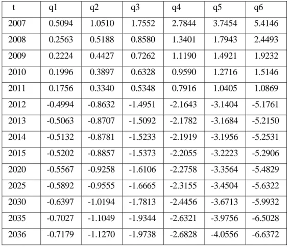
The first simulation that was run involved a 10% tax increase, as of 2012, in order to support the extra cost of reimbursing the debt to the private company that executed and financed the project.
The results are presented in table 2. From 2007 to 2011, the construction period, the welfare impact is positive for all years and for all household groups, as expected. As of 2012, the repayment of the debt is initiated.
Table 2 - Equivalent Variation: Increase in Income tax by 10% t q1 q2 q3 q4 q5 q6 2007 0.5094 1.0510 1.7552 2.7844 3.7454 5.4146 2008 0.2563 0.5188 0.8580 1.3401 1.7943 2.4493 2009 0.2224 0.4427 0.7262 1.1190 1.4921 1.9232 2010 0.1996 0.3897 0.6328 0.9590 1.2716 1.5146 2011 0.1756 0.3340 0.5348 0.7916 1.0405 1.0869 2012 -0.4994 -0.8632 -1.4951 -2.1643 -3.1404 -5.1761 2013 -0.5063 -0.8707 -1.5092 -2.1782 -3.1684 -5.2150 2014 -0.5132 -0.8781 -1.5233 -2.1919 -3.1956 -5.2531 2015 -0.5202 -0.8857 -1.5373 -2.2055 -3.2223 -5.2906 2020 -0.5567 -0.9258 -1.6106 -2.2758 -3.3564 -5.4829 2025 -0.5892 -0.9555 -1.6665 -2.3155 -3.4504 -5.6322 2030 -0.6397 -1.0194 -1.7813 -2.4456 -3.6713 -5.9932 2035 -0.7027 -1.1049 -1.9344 -2.6321 -3.9756 -6.5028 2036 -0.7179 -1.1270 -1.9738 -2.6828 -4.0556 -6.6372
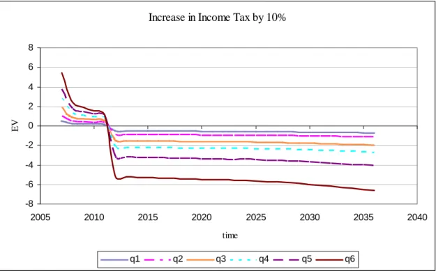
The increase in income tax adversely affects the households as it curtails the spending and leads to a substantial fall in the GDP as compared to other scenarios. The improvement of the current account balance captured by the excess of exports over imports is insufficient to compensate for the fall in GDP. The fall in output is accompanied with a rise in unemployment and falling wages. Thus an overall reduction in the incomes is largely responsible for the lower welfare.
Increase in Income Tax by 10% -8 -6 -4 -2 0 2 4 6 8 2005 2010 2015 2020 2025 2030 2035 2040 time E V q1 q2 q3 q4 q5 q6 5.2 Cut in Transfers by 10%
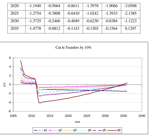
There is no policy change in the initial years till 2011, the welfare gains remain exactly the same as in Table 2. Marginal adverse impacts start as the road payments begin. Since the government expenditures fall on account of the payments and that the households receive less is a contributor to the fall in EV. The cut in expenditure leads to a fall in the GDP and since the foreign transfers are fixed, only the current account changes. The model adjusts with an increase in exports as compared to imports thus improving the current account balance with respect to the US, ROW and the EU. This export lead growth however is insufficient to compensate for the falling GDP on account of reduced expenditure and transfers by the government. As the economy grows, the share of the fixed repayments in the GDP falls and the export lead growth contributes, albeit marginally to a positive welfare of the richer households. Also the repayment amount in the latter years is a smaller fraction of the government expenditure and thus growth contributes to alleviating the decrease in welfare.
Table 3: Equivalent Variation: Cut in transfers by 10% t q1 q2 q3 q4 q5 q6 2012 -1.0572 -0.6237 -1.0670 -1.7617 -2.3952 -3.9746 2013 -1.0741 -0.6125 -1.0478 -1.7264 -2.3500 -3.8879 2014 -1.0910 -0.6004 -1.0266 -1.6883 -2.3001 -3.7932 2015 -1.1079 -0.5872 -1.0037 -1.6472 -2.2457 -3.6907
2020 -1.1940 -0.5064 -0.8611 -1.3978 -1.9066 -3.0588 2025 -1.2754 -0.3808 -0.6410 -1.0242 -1.3933 -2.1385 2030 -1.3725 -0.2466 -0.4049 -0.6230 -0.8384 -1.1223 2035 -1.4778 -0.0812 -0.1143 -0.1303 -0.1564 0.1297 Cut in Transfers by 10% -6 -4 -2 0 2 4 6 2005 2010 2015 2020 2025 2030 2035 2040 time E V q1 q2 q3 q4 q5 q6
5.3 Decrease in transport Margins by 10%
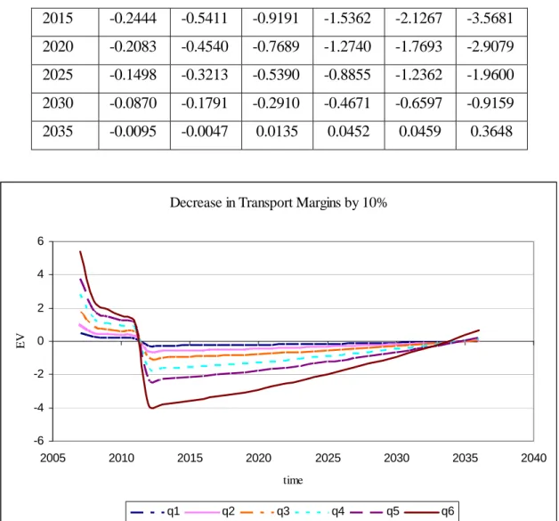
The main objective of the private-public co-operative enterprise in building the new road was to improve transportation and cut commuting time. This is modelled through a reduction in the transport margins to all agents in the economy via an ad-hoc 10% reduction in the margins. Initially the fall in transport margins is insufficient to prevent a reduction in welfare as the payments start but with progress of time, the improvement in the current account balance leads to greater savings and growth. Also the absence of adverse instruments like increase in income tax or cut in transfers that curtail spending, the growth in GDP leads to a fall in unemployment and the results are marginally better than those from the cut in transfers.
Table 4: Equivalent Variation: Decrease in transport Margins by 10% t q1 q2 q3 q4 q5 q6 2012 -0.2595 -0.5810 -0.9860 -1.6575 -2.2866 -3.8697 2013 -0.2550 -0.5687 -0.9656 -1.6200 -2.2380 -3.7770 2014 -0.2500 -0.5554 -0.9433 -1.5796 -2.1847 -3.6765
2015 -0.2444 -0.5411 -0.9191 -1.5362 -2.1267 -3.5681 2020 -0.2083 -0.4540 -0.7689 -1.2740 -1.7693 -2.9079 2025 -0.1498 -0.3213 -0.5390 -0.8855 -1.2362 -1.9600 2030 -0.0870 -0.1791 -0.2910 -0.4671 -0.6597 -0.9159 2035 -0.0095 -0.0047 0.0135 0.0452 0.0459 0.3648
Decrease in Transport Margins by 10%
-6 -4 -2 0 2 4 6 2005 2010 2015 2020 2025 2030 2035 2040 time E V q1 q2 q3 q4 q5 q6
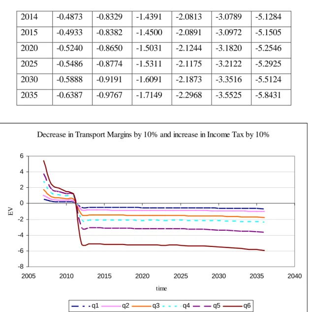
5.4 Decrease in transport Margins by 10% and Increase in Income taxes by 10% In the above scenarios we have separately simulated a fall in transport margins in addition to cut in taxes and transfers. However once the road has been completed, the benefits of a fall in transport margins will accrue. The government if so wishes then can choose to impose either additional taxes or cur transfers to meet its payment obligations. Thus the negative impacts of taxes and transfer cuts are over estimated. In the following simulations we combine the tax increase and transfer cuts with the accrued benefits of transport margins. As expected the welfare losses are lower when the implicit gains from road construction are accounted for but are not large enough to offset the additional payment burden.
Table 5: Equivalent Variation: Decrease in transport Margins by 10% and Increase in Income taxes by 10%
t q1 q2 q3 q4 q5 q6 2012 -0.4752 -0.8220 -1.4165 -2.0642 -3.0390 -5.0801 2013 -0.4813 -0.8275 -1.4280 -2.0730 -3.0596 -5.1051
2014 -0.4873 -0.8329 -1.4391 -2.0813 -3.0789 -5.1284 2015 -0.4933 -0.8382 -1.4500 -2.0891 -3.0972 -5.1505 2020 -0.5240 -0.8650 -1.5031 -2.1244 -3.1820 -5.2546 2025 -0.5486 -0.8774 -1.5311 -2.1175 -3.2122 -5.2925 2030 -0.5888 -0.9191 -1.6091 -2.1873 -3.3516 -5.5124 2035 -0.6387 -0.9767 -1.7149 -2.2968 -3.5525 -5.8431
Decrease in Transport Margins by 10% and increase in Income Tax by 10%
-8 -6 -4 -2 0 2 4 6 2005 2010 2015 2020 2025 2030 2035 2040 time E V q1 q2 q3 q4 q5 q6
5.5 Decrease in transport Margins by 10% and Decrease in transfers by 10%
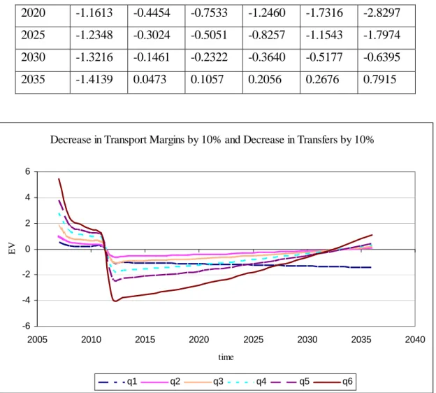
We assume that the benefits of reduction in transport margins of 10% accrue to all, but now reduce transfers by 10% to meet the cost of the road. As expected the poorest (q1 households) are affected as transfers form a larger part of their income, while the rich (q6) are not so greatly affected. This is ofcourse better than the case where we did not consider a reduction in transport costs, but just analysed the road as another investment expenditure by the government on a public good like a school or hospital.
Table 6: EV for Decrease in transport Margins by 10% and Decrease in transfers by 10% t q1 q2 q3 q4 q5 q6 2012 -1.0331 -0.5825 -0.9884 -1.6616 -2.2938 -3.8789 2013 -1.0491 -0.5692 -0.9664 -1.6211 -2.2410 -3.7780 2014 -1.0651 -0.5550 -0.9423 -1.5775 -2.1832 -3.6685 2015 -1.0811 -0.5396 -0.9162 -1.5306 -2.1203 -3.5505
2020 -1.1613 -0.4454 -0.7533 -1.2460 -1.7316 -2.8297 2025 -1.2348 -0.3024 -0.5051 -0.8257 -1.1543 -1.7974 2030 -1.3216 -0.1461 -0.2322 -0.3640 -0.5177 -0.6395 2035 -1.4139 0.0473 0.1057 0.2056 0.2676 0.7915
Decrease in Transport Margins by 10% and Decrease in Transfers by 10%
-6 -4 -2 0 2 4 6 2005 2010 2015 2020 2025 2030 2035 2040 time E V q1 q2 q3 q4 q5 q6
To have a meaningful comparison across scenarios, we compare the net present value of the equivalent variation for all the scenarios mentioned. The results substantiate the intuition where in the reduction in welfare is the least without any additional burden. The welfare loss increases with cut in transfers and is maximum for the increase in income tax. These effects are mitigated due to the presence of the reduction in transport margins on account of the new road. The poorest strate of society (q1 households) are susceptible to cut in transfers while the richest (q6 households) are adversely affected by the rise in income taxes.
Table 7 – NPV of Equivalent Variation
t q1 q2 q3 q4 q5 q6 Scenario 1 -0.5270 -1.3131 -2.2824 -4.1169 -5.9824 -11.6538 Scenario 2 -3.7536 -5.8508 -10.3646 -14.1031 -21.5646 -37.3068 Scenario 3 -9.1277 -1.7685 -3.0825 -5.1900 -7.1738 -12.9613 Scenario 4 -3.4499 -5.2783 -9.3548 -12.6589 -19.8681 -34.9884 Scenario 5 -8.8241 -1.1946 -2.0700 -3.7424 -5.4726 -10.6356 Scenario 1: Decrease in transport margins on account of new road
Scenario 2: Increase in tax rates by 10%
Scenario 3: Decrease in transfers to households by 10%
Scenario 4: Decrease in transport margins and increase in tax on households by 10% Scenario 5: Decrease in transport margins and decrease in transfers to households by 10%
6 Conclusion
The current paper set out to measure the welfare impact of the construction of a road under a public/private partnership in the Azores. The issue facing the government was not to gage the willingness to pay for a new road but to create infrastructure. Hence individuals had no choice between a road with and without toll, whose pricing would have been based on marginal cost principles. The next question then was to address the issue of the cost of infrastructure as the burden of payment would be shifted across time. Since the road introduces distortions in the system, individuals use the new road based on their propensities to consume transport services. Since the model does not factor in externalities like reduced commuting time, lower fuel expenditure and emissions and less maintenance costs, the positive welfare impacts are understated. Also on the production side, the expenditure is specifically in the road sector and thus affects the return to capital only in the road sector. The model behaviour would suggest an increased return to capital in the construction sector on account of demand for road services and thus distort the results in favour of additional capital in the construction sector. In reality the foreign firms have already invested in capital and do not incur expense on capital expenditure. To neutralise this effect the model incorporates the additional expenditure on the road as a general increase in expenditure by the government on savings.
The main concern here was to analyse the welfare impact of the project as it impacted on the equivalent variation. As expected, the project has an initial positive impact given that, during the first five years, there are no payments made to the private partner. The negative impact sets in after construction is completed and the investment has to be repaid. Account is taken of the fact that trade margins should be reduced because of improvement of land transportation.
Overall, it does not seem that the initial positive impacts on welfare compensate the subsequent welfare loss due to the payments that have to be made either through additional taxes or through reductions in transfers from the public budget to the private sector.
There is an unambiguous fall in welfare by the imposition of an additional income tax. We recommend that the best policy instrument available at the hands of the government is to
reduce the transfers to the households to pay for the road. The trade off between efficiency and equity persists and one has to sacrifice equity for the sake of efficiency.
References
Adelman, I., Robinson, S. (1989). Income distribution and development. In H. Chenery T. N. Srinivasan (Eds.), Handbook of development economics, vol. 2 (pp. 949-1003). Amsterdam: North-Holland.
Bröcker J, (2002) . Spatial Effects of European Transport Policy: A CGE Approach, in GJD Hewings, M. Sonis, D Bpyce (Eds.) Trade Networks and Hierarchies – Modelling Regional and inter regional Economies. Springer, Berlin, Heidelberg, New York, 2002, pp 11-28
Bröcker J, (2001) Trans European Effects of “Trans-European Networks”, in F Bolle and M. Carlberg (Eds.) Advances in Behavioural Economics, Essays in Honour of Horst Todt. Physica Heidelberg, 2001, pp 141-157
Dervis, K., De Melo, J., Robinson, S. (1982). General equilibrium models for
development policy. Cambridge, UK: Cambridge University Press.
Dixon, P.B., Rimmer, M.T. (2002). Dynamic general equilibrium modeling for forecasting and policy: A practical guide and documentation of MONASH. In R. Blundell, R. Caballero, J.-J. Laffont T. Persson (Eds.), Contributions to economic
analysis, vol. 256. Amsterdam: North-Holland.
Fortuna Mário, Bayar Ali, Mohora Cristina, Opese Masudi, Sisik Suat (March 2009) Azormod Dynamic General Equilibrium Model for Azores CEEAplA WP No. 02/2009 http://www.uac.pt/~ceeapla/pt/pdf/papers/Paper02-2009.pdf
Harrison, G.W., Kriström, B. (1997). General equilibrium effects of increasing carbon
taxes in Sweden.
Heer Burkhard, Maussner Alfred (2005) Dynamic General Equilibrium Modelling:
Computational Methods and Applications, Springer
Löfgren, H., Harris, R. L., Robinson, S. (2002). A standard computable general equilibrium (CGE) in GAMS. IFPRI, Microcomputers in Policy Research, 5. Rosenthal, R.E. (2006). GAMS – A user’s guide. Washington: GAMS Development
Corporation.
Sanz-de-Galdeano, A., Turunen, J. (2006). The euro area wage curve. Economics
Letters, 92, 93-98.