Multi-Objective Forest Vehicle Routing Using Savings-Insertion
and Reactive Tabu with a Variable Threshold
Moussa Sinsé Bagayoko*, Thien-My Dao*, Barthélemy Ateme-Nguema**
*(École de technologie supérieure, Mechanical Engineering Department, Montreal, Canada** (Université du Québec en Abitibi-Témiscamingue, Management Sciences Department, Rouyn-Noranda, Canada
ABSTRACT
This paper focuses on how the competitiveness of forestry companies in Canada is impacted by forest products distribution and transportation costs, especially in the context of exports. We propose a new two steps approach, consisting in building a good initial solution and then improving it to solve multi-objective forest vehicle routing problem. The main objective of this paper is to solve a multi-objective forest vehicle routing problem using the Savings-insertion, followed by the Reactive tabu, with a variable threshold. To that end, first, a mathematical model is established; secondly, our new Savings-insertion builds a good initial solution, and thirdly, our new Reactive tabu with a variable threshold improves the initial solution. The three main objectives are the minimization of number of routes, the minimization of total distance and the minimization of total time by respecting the specified time window and the demand of all customers, which are sometimes important in this field. Finally, the experimental results obtained with our methodology for the named vehicle routing problem are provided and discussed.
Keywords:
Forest transportation, multi-objective, reactive tabu, time windows, vehicle routingI.
INTRODUCTION
Forest product distribution is a process by which forest products are moved from sources to customers. The increase of distance between forest areas and mills causes a considerable in-crease in forest companies’ transportation costs. According to [1], transportation costs typically represent 10-20% of the final price of goods on the market; ref. [2] point out that in Quebec, transportation accounts for over 30% of provisioning costs for wood transformation mills, i.e., approximately $15 per cubic meter of round wood. The average distance between forest areas where wood is collected and mills to which the wood is transported is around 150 km, and about 50% of the fuel required per cubic meter of wood collection is consumed by forest trucks traveling, half of the time empty, between forest areas and mills.
According to [3], in countries like Chile, Canada, Sweden, Finland and New Zealand, the forest industry is mainly dependent on exports. According to [4], Canada is the largest exporter of forest products in the world, with $31 billion in sales in 2014. The sector thus ranks second in exports after the oil and gas sector, accounting for almost 6% of all Canadian exports in 2014. Secondly, according to [5] and [6], transportation costs account for a great portion of the total cost of forest operation. Thirdly, according to [3], to be competitive, the forest industry must maintain or improve the effectiveness of all its operations.
Over the past 20 years, the Vehicle Routing Problem (VRP) was mainly solved through the use of meta-heuristics (see [7] and [8]). Ref. [9] carried out a taxonomic review of VRP characterizing this
research field, and conducted a detailed
classification of variants with many examples. Following the review of previous classifications and taxonomies, major journals having published articles on the subject issue are listed, and a taxonomy is proposed. They conducted a classification by type of
study, scenario characteristics, physical
characteristics of the problem, and by characteristics of information and data used. Ref. [10] in turn
conducted a review of biologically-inspired
algorithms used to handle the VRP. He highlighted the different variants of the problem and the different methodologies used to solve them. These include evolutionary algorithms, ant colonies, particle swarm optimization, neural networks, artificial immune systems and hybrid algorithms. Ref. [11] for their part conducted a review of the state of the art of large scale VRP, indicating the difficulty of solving the problems of more than 100 customers with exact methods. They criticized the major works on large scale VRP by highlighting the techniques used. The review compared the performance of different algorithms and conducted an analysis based on key attributes such as effectiveness, efficiency, simplicity, and flexibility.
Ref. [12] proposed a model of long-haul VRP and scheduling integrating working hour’s rules. The
resolution method used was a bi-objective tabu search algorithm. The first objective is to minimize the total number of vehicles used, and the second, to minimize the total cost, which is the weighted sum of the total distance traveled and the corresponding total time. Ref. [13], based on the work of [12], established a multi-criteria optimization model of long-haul VRP and scheduling integrating working hours rules. The solution method used was a bi-objective tabu search algorithm determining a set of heuristic non-dominated solutions. The mechanism consists of a single thread in which the weights assigned to the two objectives, namely, operating costs and driver inconvenience, are dynamically modified, and in which dominated solutions are eliminated throughout the search. Ref. [14] proposed a multi-depot VRP with a simultaneous delivery and pick-up model. The resolution method used was the
iterated local search embedded adaptive
neighborhood selection approach. Ref. [15] tested local search move operators on the VRP with split deliveries and time windows. To that end, they used eight local search opera-tors, in combinations of up to three of them, paired with a max-min ant system.
Ref. [16] developed a dynamic model for
solving the mixed integer programming of forest plant location and design, as well as production levels and flows between origins and destinations.
Ref. [17] proposed a multi-depot forest
transportation model solving the tactical problem of the flow between origins and destinations without solving the operational problem of VRP. The solution method used was column generation. Ref. [6] proposed a model for forest transportation, solving the problem of flow between origins and
destinations, and involving a sedimentation
constraint. They did not address the VRP, and ignored the time windows constraint for customers. The resolution method used was the ant colony algorithm. Ref. [18] established a bi-level model using a genetic algorithm to solve the problems of locating and sizing mills and of transporting forest products. In their model, individual members of the initial population are found by solving the lo-cation and size of plants, at which point the VRP is solved for each individual. The authors do not integrate the time windows constraint for customers. Ref. [19] proposed a multi-depot forest transportation model. The resolution method they used involved the generation of transport nodes by solving the linear programming problem of flow distribution and routing of these nodes using a tabu search. Ref. [20] developed two linear programming models of planning for collaborative forest transportation for eight companies in the south of Sweden. The first model was based on the direct flow between supply and demand points, while the second one included backhauling. According to the authors, in the
Swedish forest industry, transportation costs represent approximately one-third of total raw material costs. According to [21], the Vehicle Routing Problem is assimilated to an extension of the traveling salesman problem. According to [22], this problem is known as a NP-complete problem. Therefore, the Vehicle Routing Problem is NP-complete.
Unlike other authors making an arbitrary hierarchy of optimality criteria, we evaluate them all
simultaneously. This simultaneous evaluation
provides good solutions least questionable. It is done by minimizing the total cost which is an aggregation of costs due to different optimality criteria: the number of vehicles, the total distance and total travel time. The goal of this paper is to present a new two steps resolution approach for the Multi-Objective Forest Vehicle Routing Problem (MOFVRP). Our main contribution is the establishment of Savings-insertion heuristic for generating initial solution and the establishment of Reactive tabu with a variable threshold improving the solution. Applying our methodology to a practical case shows its effectiveness in solving concrete problems. This methodology clearly provides the best compromise solution for the forest transportation optimization problem, independently of parameters.
In the next section, we explain our methodology: first, we describe the problem and pro-pose our mathematical model; secondly, we show our global methodology; thirdly, we establish our Savings-insertion heuristic, and fourthly, we establish our Reactive tabu with a variable threshold meta-heuristic. In the third section, we present our results, followed by a discussion, and finally, we end with a conclusion in the fourth section.
II.
METHODOLOGY
2.1. Problem description and mathematical model
To perform an MOFVRP optimization, we
propose an optimization based on Savings-insertion, followed by the Reactive tabu with a variable threshold. This allows the minimization of the total transport cost, including hard capacity and hard time windows. Below, we present our improved and
completed mathematical model (see [23], [24] and
[25]).
Let us assume that m vehicles, with a load
capacity of Q, are needed. There are L customers
and one depot, which takes the index 1 at the start of
the route and the index L+2 at the route end. The
fleet is homogeneous, and every customer demand must be satisfied within his time window. We split every customer having a demand upper than the vehicles’ load capacity to get each customer demand
lower than or equal to the vehicles’ load capacity.
Assumptions
a. Each customer location (xj, yj), demand qj, and
time window (tsj = start time, tej = end time) are
known;
b. Each customer is served only by one vehicle at a
time;
c. Each vehicle leaves the depot (index 1) and
returns to the depot (index L+2);
d. All vehicles needed are immediately available;
e. The average vehicle moving speed VS is known;
f. Each customer demand qj is lower than or equal
to vehicles’ load capacity Q.
Notation
xj, yj customer j location
tsj customer j start time
te
j customer j end time
qj customer j demand
Ct total transport cost
m number of vehicles used
VS average moving speed of vehicles
Q vehicles’ load capacity
L number of customers
cf unit vehicle fixed cost, covering loading
and unloading
cijk unit transport cost per kilometer of vehicle
k from i to j
dij distance between two locations i and j
xijk indicates if vehicle k goes from i to j
cvt unit route time cost of vehicle
cdt unit work time cost of driver
tjk arrival time of vehicle k to customer j
wjk waiting time for vehicle k at customer j
sj customer j service time
tij time spent from i to j
yjk indicates if customer j is served by vehicle
k
Tk end of vehicle k time
The studied problem is modeled and the mathematical model objective is given in (1):
1 2
1 2 1
1 2
1 2 1
m i n
( ) ( )
L L m
t f ijk ij ijk
i j k
L L m
v t d t ijk ij jk j
i j k
C m c c d x
c c x t w s
(1)This objective function is the total transport cost, where the first element is the total fixed vehicle cost, the second is the total distance cost summation, and the third is the total vehicle route time cost and total driver work time cost summations. This aggregation permits to find a trade-off between three objectives: the minimization of numbers of vehicle, the minimization of total distance traveled and the
minimization of total time spends to travel. The time spent going from i to j is:
/ 1, 1 , 2 , 2
ij ij
t d V S i L j L (2)
The waiting time for vehicle k at customer j is:
m a x ( s , 0 ) j 2 , 2 , 1,
jk j jk
w t t L k m (3)
There are eleven constraints restrictions:
The (4) is the first constraint, and imposes the
condition that the variable yjk be binary. The (5) is
the second constraint, and imposes the condition that
the variable xijk be binary.
1,0 ,
th e cu sto m er j is served b y th e veh icle k jk o th erw ise
y (4)
1, 0 ,th e v e h ic le k g o e s fro m i to j ijk o th e rw ise
x (5)
The (6) is the third constraint, and imposes the condition that every vehicle leaves the depot (index
1). The (7) is the fourth constraint, and imposes the
condition that every vehicle returns to the depot
(index L+2).
1 1 m k k y m
(6) 2
1 m
L k
k
y m
(7)The (8) is the fifth constraint, and imposes the condition that every customer be served only by one vehicle. The (9) is the sixth constraint, and for each customer j, it means that the customer is served only by one vehicle passing through only one other customer. The (10) is the seventh constraint, and
indicates that the total load for vehicle k cannot
exceed the vehicles’ load capacityQ.
1
1 2 , 1
m
jk k
y j L
(8)
1 12 , 1 , 1,
L
ijk jk
i
x y j L k m
(9) 1 2 1, L j jk jq y Q k m
(10)The (11) is the eighth constraint, and gives the
relation between vehicle k arrival time to the
customer i and its arrival time to customer j. The
(12) is the ninth constraint, and indicates that the
service at customer j must begin before Tk, the end
of the vehicle k time.
( ) 1, 1 , 2 , 2 , 1,
jk ijk ik ik i ij
t x t w s t i L j L k m (11)
2 , 2 , 1,
jk jk k
t w T j L k m (12)
The (13) is the tenth constraint, and indicates that no customer can be served before his start time. The (14) is the eleventh constraint, and indicates that no customer can be served after his end time.
2 , 2 , 1,
s
jk jk j
t w t j L k m (13)
2 , 2 , 1,
e
jk jk j
These eleven constraints restrictions allow the realization of the objective of minimizing the total transport cost by obtaining a feasible solution directly. In the next subsection, we explain the new global methodology proposed to solve this mixed-integer linear programming problem.
2.2. Global methodology
The proposed approach to solving the
MOFVRP consists of two steps. The initial solution technique for the MOFVRP based on the Savings-insertion technique for generating the initial solution is developed (Fig. 2) in order to serve as the starting point of our improvement technique. The improvement technique for MOFVRP developed is based on a Reactive tabu with a variable threshold,
and is used to improve the initial solution (Fig. 3).
This allows us to find the best compromise (optimal) solution of the problem. The different steps of the global methodology are presented in Fig. 1. In the next subsection, we propose and present our initial Savings-insertion solution technique.
Start FVRP solving global methodology
Initialize Savings-insertion parameters Import FVRP data
Apply Savings-Insertion for generating FVRP initial solution S
Apply Reactive tabu with a variable threshold for FVRP optimization
Stop FVRP solving global methodology
Initialize Reactive tabu with a variable threshold parameters, Best solution Sbest = Initial solution S
Export FVRP two best solutions
Figure 1: global methodology
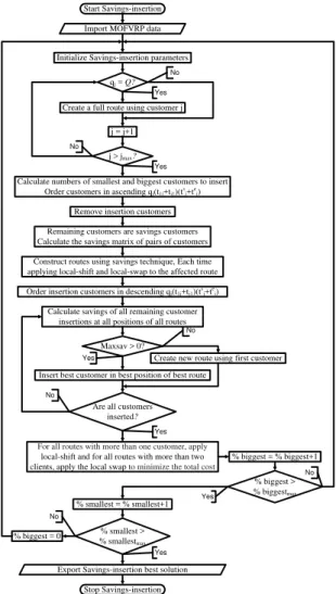
2.3.Initial solution by Savings-insertion heuristic
The VRP is one of the most studied combinatorial problems in operations research. The well-known [26] saving algorithm, which formed the basis for many other solving algorithms for the capacitated VRP, is a very fast and simple algorithm for solving the VRP. Ref. [27] provided the historical background for the development of the savings method, and subsequently proposed variations to the basic savings formula and other
improvements. Ref. [28] proposed a new way of
merging routes and a corresponding formula for
calculating savings. They applied the method and developed a new heuristic that dynamically
recalculates savings during iterations. Based on [26]
saving algorithm, a Savings-insertion technique is proposed for generating the initial solution. Our first
main algorithm is presented in Fig. 2.
Start Savings-insertion
Initialize Savings-insertion parameters Import MOFVRP data
Calculate numbers of smallest and biggest customers to insert Order customers in ascending qj(t1j+tj1)(tsj+tej)
Insert best customer in best position of best route j > jmax?
Yes No
Remove insertion customers
Remaining customers are savings customers Calculate the savings matrix of pairs of customers
Order insertion customers in descending qj(t1j+tj1)(tsj+tej) Construct routes using savings technique, Each time applying local-shift and local-swap to the affected route
Maxsav > 0?
Yes
No
Create new route using first customer qj = Q?
Yes No
Create a full route using customer j
j = j+1
For all routes with more than one customer, apply
local-shift and for all routes with more than two clients, apply the local swap to minimize the total cost
Are all customers inserted?
Yes No
Stop Savings-insertion Export Savings-insertion best solution Calculate savings of all remaining customer
insertions at all positions of all routes
% smallest > % smallestmax
Yes No
% smallest = % smallest+1
% biggest > % biggestmax Yes
% biggest = % biggest+1
% biggest = 0
No
Figure 2: savings-insertion for generating the initial solution
This Savings-insertion technique extends the [26] savings heuristic by adding the insertion of smallest customers (using a percentage of smallest customers) and biggest customers (using a percentage of biggest customers) according to the value of qj(t1j+tj1)(tsj+tej). In the next subsection, we
propose and explain our new Reactive tabu with a variable threshold.
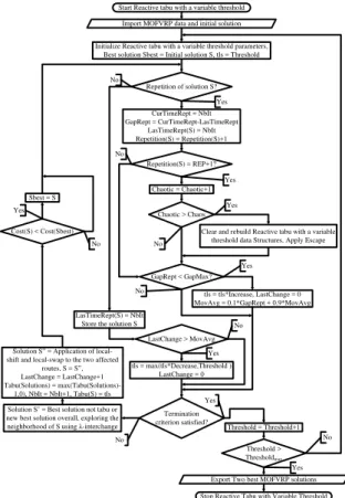
2.4.Improvement by Reactive tabu with a variable threshold meta-heuristic
It is known that the weakness of neighborhood search algorithms lies their possible trap into local optima. Our second main algorithm is
presented in Fig. 3. This Reactive tabu with a
variable threshold algorithm is an extension of the
extension is done by adding a parameter for setting a minimum value of the tabu list size tls called
Threshold.The variation of this parameter improves the exploration of the search space by varying the compromise between intensification and diversification. It allows us to get a dynamic
compromise between intensification and
diversification. In summary, the more the same solutions found are repeated, the more the tabu list size increases, and vice versa; conversely, the more the solutions are different, the more the tabu list size decreases. This mechanism whereby the number of tabu solutions is increased when reaching local
optima allows us to avoid the local optima trap by exploring other solutions in this case because all
neighbors have become tabu. The optimization
technique for the Reactive tabu with a variable
threshold aimed at improving the initial solution
(improvement) is developed (Fig. 3) in order to find the best compromise (optimal) solution of the problem. It can quickly check the feasibility of the movement suggested, and then react to the repetition to guide the search. This algorithm is performed via a tabu list size (tls) update mechanism elaborated in five steps, as shown in Fig. 3. The counters and parameters used in Reactive tabu with a variable threshold are defined as follows, and initialized to the following values.
Minimum of tabu list size (tls) value: Threshold
= 1 to 10
Counter for often-repeated sets of solutions:
Chaotic = 0
Moving average for the detected repetitions:
MovAvg = 0
Gap between two consecutive repetitions:
GapRept = 0
Number of iterations since the last change in tls
value: LastChange = 0
Iteration number when an identical solution was
last noticed: LasTimeRept = 0
Iteration number of the most recent repetition:
CurTimeRept = 0
Maximum limit for often-repeated solutions:
REP = 5
Maximum limit for sets of often-repeated
solutions: Chaos = 5
Increase factor for the tabu tenure value:
Increase = 2
Decrease factor for the tabu tenure value:
Decrease = 0.5
The constant used for comparison with GapRept
to get the moving average: GapMax = 100.
According to [30], “The λ-interchange
method is based on the interchange of customers between sets of routes. This technique generation mechanism can be described as follows. Given a solution to the problem represented by the set of
routes S = {R1,…,Rp,…,Rq,…,Rk}, where each route
is the set of customers serviced on this route, a λ
-interchange between Rp and Rq is the replacement of
a subset of customers S1 ⊆ Rp of size |S1| ≤ λ by
another subset S2 ⊆ Rq of size |S2| ≤ λ, and
vice-versa, to get two new routes R’p= (Rp - S1) + S2 and
R’q= (Rq - S2) + S1 and a new neighboring solution
S’ = {R1,…,R’p,…,R’q,…,Rk}”. In this work, we
limited ourselves to sequences of consecutive
customers. The neighborhood Nλ(S) of a given
solution S is the set of all neighbors S' generated in
this manner for a given value of λ. We established
our 1-interchange+ by adding the operators (2, 1)
and (1, 2) to 1-interchange. Thus, we can more
explore the search space than the 1-interchange in less time than the 2-interchange.
Neighborhood search algorithms can fall into the local optima trap. This can be avoided by using a metaheuristic that allows non-improving moves. The tabu search is a well-known metaheuristic, and is considered by some to be the
best approach for solving VRP problems (see [31]
for further information). The Reactive tabu search
was introduced by [29], and focuses on a tabu search
component called the tabu list size (tls), often referred to as Tabu tenure, which determines how long a move can be locked up before it is allowed to reappear. The Reactive tabu search scheme uses an analogy with the theory of dynamical systems, where the tabu list size depends on the repetition of solutions, and consequently, tls is determined dynamically, as opposed to the standard version of the tabu search, where tls is fixed. Reactive tabu search employs two mechanisms, and both react to repetitions. The first mechanism is used to produce a balanced tabu list size, and consists of two reactions. A fast reaction increases the list size when solutions are repeated, while a slow reaction reduces the list size for those regions of the search space that do not need large list lengths. The second mechanism provides a systematic way to diversify the search when it is only confined to one portion of the
solution space. The experiments of [29] and [32]
showed the superiority of Reactive tabu search compared to other tabu search schemes.
Below, we present details of our Reactive tabu with a variable threshold, which dynamically
updates the value of the Tabu list size (tls),
automatically reacting to repetitions. First, our
Reactive tabu with a variable threshold extends the
Reactive tabu by adding a parameter for setting a
customers within the route, if doing so improves the solution quality. In the next section, the experimental data and results of our initial Savings-insertion solution and Reactive tabu with a variable threshold improved solution results are presented.
Start Reactive tabu with a variable threshold
Repetition of solution S?
CurTimeRept = NbIt GapRept = CurTimeRept-LasTimeRept
LasTimeRept(S) = NbIt Repetition(S) = Repetition(S)+1
Repetition(S) = REP+1?
Chaotic = Chaotic+1
Chaotic > Chaos
GapRept < GapMax?
LastChange > MovAvg
tls = max(tls*Decrease,Threshold ) LastChange = 0
Yes
Yes
Clear and rebuild Reactive tabu with a variable threshold data Structures, Apply Escape
Yes
Yes No
No
No
tls = tls*Increase, LastChange = 0 MovAvg = 0.1*GapRept + 0.9*MovAvg
Yes
No No
LasTimeRept(S) = NbIt Store the solution S
Termination criterion satisfied? No
Yes Initialize Reactive tabu with a variable threshold parameters,
Best solution Sbest = Initial solution S, tls = Threshold Import MOFVRP data and initial solution
Solution S’ = Best solution not tabu or new best solution overall, exploring the neighborhood of S using λ-interchange
Solution S” = Application of local-shift and local-swap to the two affected
routes, S = S”, LastChange = LastChange+1 Tabu(Solutions) =
max(Tabu(Solutions)-1,0), NbIt = NbIt+1, Tabu(S) = tls Cost(S) < Cost(Sbest)
Sbest = S Yes
No
Export Two best MOFVRP solutions Stop Reactive Tabu with Variable Threshold
Threshold = Threshold+1
Threshold > Thresholdmax
Yes No
Figure 3: reactive tabu with a variable threshold for improving the solution
III.
RESULTS
AND
DISCUSSION
Below on TABLE II, we present our
completed data (see [23], [24] and [25]). In our
previous works these data was adapted from [18].
The central depot, which takes the index 1 at the
start of the route and the index L+2 at the route end,
and from which all customers are served, is located at (0, 0), and is open from minutes 0 to 2400. TABLE II shows the data of each customer. The location coordinates are in kilometers; the weekly demand quantity is in cubic meters; the start and end times are in minutes. The fleet is homogeneous, and
the vehicles used have a load capacity Q of 40 cubic
meters, and an average speed VS of 60 kilometers
per hour. For cost calculations, we assume that the
unit vehicle fixed cost cf = $400, the unit transport
cost per kilometer cijk = $2.8, the unit vehicle route
time cost per minute cvt = $1.85, the unit driver work
time cost per minute cdt = $0.45. We used 50 as a
maximum percentage of smallest customers and 49
as a maximum percentage of biggest customers. Thus, at one end, we fall on savings and the other on
insertion. The distance between two locations i and j
are calculated using a symmetric problem formula:
2 2
( ) ( ) 1, 1
ij i j i j
d x x y y i a n d j L (15)
Each route duration is calculated according to [34], as follows: departure at the depot start time (ts1) and
forward scan to determine earliest finish time; reverse scan from earliest finish time to determine
the latest start time for this earliest finish time (t1k);
departure at the determined latest start time and second forward scan to delay waits as much as possible to the end of the route.
Table I: Initial Savings-insertion solution results
Savings-insertion route Cost ($)
[1, 38, 54] 1493.2
[1, 46, 54] 2865.1
[1, 5, 6, 7, 8, 9, 10, 11, 14, 54] 5109.4 [1, 16, 3, 19, 17, 18, 50, 49, 41, 40, 39, 32, 54] 6143.4 [1, 15, 2, 52, 51, 42, 54] 5991.3 [1, 13, 20, 4, 12, 54] 3404.1 [1, 24, 22, 23, 28, 27, 29, 26, 25, 44, 43, 47, 54] 7048.8 [1, 31, 37, 36, 48, 53, 35, 34, 33, 54] 3265.1
[1, 21, 45, 54] 4807.6
[1, 30, 54] 466.3
Total cost 40,594.3
1
2
3 4
5
6 7 8 10 9
11 12 13
14 15
16 17
18
19
20 21
22 23
24 25
26 27 28
29
30
31 32
33 34
35 36
37
38 39 40
41 42
43
44
45
46 47
48
49 50
51
52 53
Customer Location Demand Start time
Finish time
Service time
1 0 0 0 0 2400 0
2 50 -290 29.379 0 960 10
3 -120 -250 3.711 0 960 10
4 -90 -250 23.664 0 960 10
5 -145 -320 4.79 0 960 10
6 -100 -390 4.517 0 960 10
7 -80 -390 2.018 0 960 10
8 -82 -337 1.57 0 960 10
9 -40 -332 5.317 0 960 10
10 -46 -324.5 13.403 0 960 10
11 -42 -286 3.725 0 960 10
12 -63 -200.5 6.676 0 960 10
13 -112.5 -199 6.78 0 960 10
14 -38 -242 4.3 0 960 10
15 9 -251 2.065 480 1440 10
16 40 -230 5.335 480 1440 10
17 -159 -108 3.797 480 1440 10
18 -211 -126 0.856 480 1440 10
19 -142 -163 5.631 480 1440 10
20 -121 -242 1.496 480 1440 10
21 -124 -213 24.741 480 1440 10
22 -61 -6 3.464 480 1440 10
23 -79 -11 3.691 480 1440 10
24 -51 14 1.293 480 1440 10
25 -117 18 7.899 480 1440 10
26 -126 -8 2.255 480 1440 10
27 -88 -28 2.664 480 1440 10
28 -95 -9 1.504 960 1920 10
29 -112 -54 0.859 960 1920 10
30 3 -3 8.319 960 1920 10
31 38 -29 1.299 960 1920 10
32 -35 -41 1.715 960 1920 10
33 -5 39 1.535 960 1920 10
34 46 48 6.198 960 1920 10
35 91 52 18.079 960 1920 10
36 187 47 2.008 960 1920 10
37 225 19 1.692 960 1920 10
38 -40 -97 40 960 1920 10
39 -40.001 -96.999 4.018 960 1920 10
40 -90 -100 6.067 960 1920 10
41 -83 -118 0.539 1440 2400 10
42 0.5 -117 2.432 1440 2400 10
43 -180 468 1.978 1440 2400 10
44 -106 126 7.446 1440 2400 10
45 -269 81 11.174 1440 2400 10
46 34 237 40 1440 2400 10
47 34. 001 236.999 3.413 1440 2400 10
48 149.5 45 0.744 1440 2400 10
49 -195 -198 2.103 1440 2400 10
50 -200 -207 1.829 1440 2400 10
51 -52 -231 0.676 1440 2400 10
52 5 -446 3.978 1440 2400 10
53 109.5 38 3.116 1440 2400 10
54 0 0 0 0 2400 0
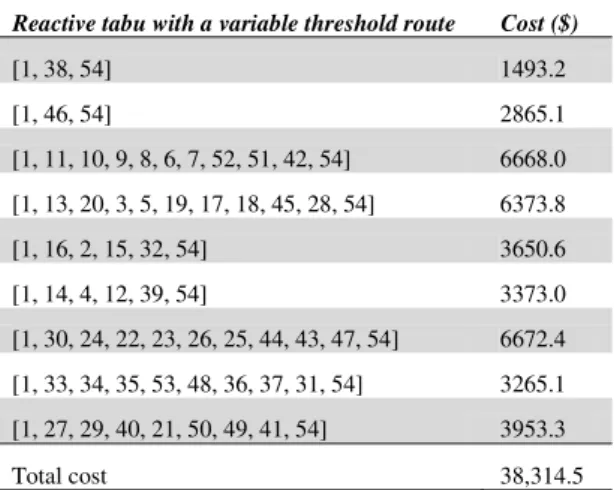
Table III: Final reactive tabu with a variable threshold solution results
Reactive tabu with a variable threshold route Cost ($)
[1, 38, 54] 1493.2
[1, 46, 54] 2865.1
[1, 11, 10, 9, 8, 6, 7, 52, 51, 42, 54] 6668.0 [1, 13, 20, 3, 5, 19, 17, 18, 45, 28, 54] 6373.8 [1, 16, 2, 15, 32, 54] 3650.6 [1, 14, 4, 12, 39, 54] 3373.0 [1, 30, 24, 22, 23, 26, 25, 44, 43, 47, 54] 6672.4 [1, 33, 34, 35, 53, 48, 36, 37, 31, 54] 3265.1 [1, 27, 29, 40, 21, 50, 49, 41, 54] 3953.3
Total cost 38,314.5
1
2 3 4
5
6 7 8 10 9
11 12 13
14 15
16 17
18 19
20 21
22 23
24 25 26 27 28 29
30 31 32
33 34
35 36 37
38 39 40
41 42 43
44 45
46 47
48
49 50
51
52 53
Figure 5: final reactive tabu with a variable threshold solution graphic
0 100 200 300 400 500 600 700 3.8
3.85 3.9 3.95 4 4.05x 10
4
Figure 6: final reactive tabu with a variable threshold convergence graphic
TABLE I shows initial MOFVRP solution
results generated by Savings-insertion. Each route’s
customers and cost are given, and the total cost is calculated. It is a ten-route solution having a total cost of $40,594.3. The corresponding total distance and total route duration are respectively 6731.8 kilometers and 7715.4 minutes. Fig. 4 shows the initial MOFVRP solution location sequences graphic. For example, the route [1, 31, 37, 36, 48, 53, 35, 34, 33, 54] to the right in this figure means
that the vehicle leaves the depot (index 1), goes
distance and total route duration are respectively 6406.2 kilometers and 7294.4 minutes. Fig. 5 shows the final MOFVRP solution location sequences graphic. Fig. 6 shows the Reactive tabu with a variable threshold MOFVRP convergence graphic; it shows the number of iterations at which the best
solution is reached. This methodology clearly
provides the best compromise solution for the
MOFVRP optimization, independently of
parameters.
IV.
CONCLUSION
In our paper, we resolved a practical
MOFVRP using our approach based on
Savings-insertion, followed by the Reactive tabu with a variable threshold. To that end, we used our mathematical model to minimize the total transport cost, including hard capacity and hard time windows
constraints. Our results show that minimizing the
total cost, our methodology clearly provides the best compromise solution, independently of parameters. We then conclude that Savings-insertion, followed by the Reactive tabu with a variable threshold is a promising approach, which will be used in our future research to further explore the MOFVRP.
References
[1] Toth, P., and D. Vigo. 2001. “The vehicle
routing problem”.
[2] El Hachemi, Nizar, Michel Gendreau and
Louis-Martin Rousseau. 2013. “A heuristic to
solve the synchronized log-truck scheduling
problem”. Computers & Operations
Research, vol. 40, No. 3, pp. 666-673.
[3] Rönnqvist, M. 2003. “Optimization in
forestry”. Mathematical programming, vol.
97, No. 1, pp. 267-284.
[4] Natural Resources Canada (2016),
http://www.nrcan.gc.ca (last accessed on July 29, 2016).
[5] Epstein, R., M. Rönnqvist and A. Weintraub.
2007. “Forest transportation”. Handbook of
Operations Research In Natural Resources, pp. 391-403.
[6] Contreras, M.A.C.M.A., W.C.W. Chung and
G.J.G. Jones. 2008. “Applying ant colony
optimization metaheuristic to solve forest transportation planning problems with side
constraints”. Canadian Journal of Forest
Research, vol. 38, no 11, p. 2896-2910.
[7] Jozefowiez, N., F. Semet and E.G. Talbi.
2008. “Multi-objective vehicle routing
problems”. European Journal of Operational
Research, vol. 189, No. 2, pp. 293-309.
[8] Vidal, T., T.G. Crainic, M. Gendreau and C.
Prins. 2011. “Heuristiques pour les problèmes
de tournées de véhicules multi-attributs”.
[9] Eksioglu, B., A.V. Vural and A. Reisman.
2009. “The vehicle routing problem: A
taxonomic review”. Computers & Industrial
Engineering, vol. 57, No. 4, pp. 1472-1483.
[10] Potvin, J.Y. 2009. “A review of bio-inspired
algorithms for vehicle routing”. Bio-inspired
Algorithms for the Vehicle Routing Problem, pp. 1-34.
[11] Gendreau, M., and C.D. Tarantilis. 2010.
“Solving large-scale vehicle routing problems
with time windows: The state-of-the-art”.
CIRRELT.
[12] Rancourt, M.E., J.F. Cordeau and G. Laporte.
2012. “Long-haul vehicle routing and
scheduling with working hour rules”.
Transportation Science.
[13] Rancourt, Marie‐ Eve, and Julie Paquette.
2014. “Multicriteria Optimization of a
Long‐ Haul Routing and Scheduling
Problem”. Journal of Multi‐ Criteria
Decision Analysis, vol. 21, No. 5-6, pp. 239-255.
[14] Li, Jian, Panos M Pardalos, Hao Sun, Jun Pei
and Yong Zhang. 2015. “Iterated local search embedded adaptive neighborhood selection approach for the multi-depot vehicle routing problem with simultaneous deliveries and
pickups”. Expert Systems with Applications,
vol. 42, No. 7, pp. 3551-3561.
[15] McNabb, Marcus E, Jeffery D Weir,
Raymond R Hill and Shane N Hall. 2015. “Testing local search move operators on the vehicle routing problem with split deliveries
and time windows”. Computers & Operations
Research, vol. 56, pp. 93-109.
[16] Troncoso, J.J., and R.A. Garrido. 2005.
“Forestry production and logistics planning:
an analysis using mixed-integer
programming”. Forest Policy and Economics,
vol. 7, No. 4, pp. 625-633.
[17] Carlsson, D.C.D., and Rönnqvist, M.R.M.
2007. “Backhauling in forest transportation:
models, methods, and practical usage”.
Canadian Journal of Forest Research, vol. 37, No. 12, pp. 2612-2623.
[18] Marinakis, Y., and M. Marinaki. 2008. “A
bilevel genetic algorithm for a real life
location routing problem”. International
Journal of Logistics: Research and Applications, vol. 11, No. 1, pp. 49-65.
[19] Flisberg, P., B. Lidén and M. Rönnqvist.
2009. “A hybrid method based on linear programming and tabu search for routing of
logging trucks”. Computers & Operations
Research, vol. 36, No. 4, pp. 1122-1144.
[20] Frisk, M., M. Göthe-Lundgren, K. Jörnsten
and M. Rönnqvist. 2010. “Cost allocation in
Journal of Operational Research, vol. 205, No. 2, pp. 448-458.
[21] Dhaenens, C., M.L. Espinouse and B. Penz.
2008. “Classical combinatorial problems and
solution techniques”. Operations Research
and networks, pp. 71-103.
[22] Ismail, S.B., F. Legras and G. Coppin. 2011.
“Synthèse du problème de routage de
véhicules”.
[23] Bagayoko, M., Dao, T. M., & Ateme-Nguema, B. H. (2013, October).
“Optimization of forest vehicle routing using the metaheuristics: reactive tabu search and extended great deluge”. In Industrial Engineering and Systems Management (IESM), Proceedings of 2013 International Conference on (pp. 1-7). IEEE.
[24] Bagayoko, M., Dao, T. M., & Ateme-Nguema, B. H. (2013, December). “Optimization of forest vehicle routing using reactive tabu search metaheuristic”. In 2013 IEEE International Conference on Industrial Engineering and Engineering Management (pp. 181-185). IEEE.
[25] Bagayoko, M., Dao, T. M., & Ateme-Nguema, B. H. (2015, March). “Forest vehicle routing problem solved by New Insertion and meta-heuristics”. In
Industrial Engineering and Operations Management (IEOM), 2015 International Conference on (pp. 1-8). IEEE.
[26] Clarke, G. U., and John W. Wright. 1964.
“Scheduling of vehicles from a central depot to a
number of delivery points”. Operations research,
vol. 12, No. 4, pp. 568-581.
[27] Rand, Graham K. 2009. “The life and times of the
Savings Method for Vehicle Routing Problems”.
ORiON: The Journal of ORSSA, vol. 25, No. 2.
[28] Stanojević, Milan, Bogdana Stanojević and Mirko
Vujošević. 2013. “Enhanced savings calculation
and its applications for solving capacitated vehicle
routing problem”. Applied Mathematics and
Computation, vol. 219, No. 20, pp. 10302-10312.
[29] Battiti, Roberto and Giampietro Tecchiolli. 1994.
“The reactive tabu search”. ORSA journal on
computing, vol. 6, No. 2, pp. 126-140.
[30] Thangiah, S.R., J.Y. Potvin and T. Sun. 1996.
“Heuristic approaches to vehicle routing with
backhauls and time windows”. Computers &
Operations Research, vol. 23, No. 11, pp. 1043-1057.
[31] Cordeau, Jean-François, Michel Gendreau, Gilbert
Laporte, Jean-Yves Potvin and François Semet.
2002. “A guide to vehicle routing heuristics”.
Journal of the Operational Research Society, pp. 512-522.
[32] Osman, Ibrahim H, and Niaz A. Wassan. 2002. “A
reactive tabu search meta‐ heuristic for the vehicle
routing problem with back‐ hauls”. Journal of
Scheduling, vol. 5, No. 4, pp. 263-285.
[33] Wassan, Niaz A, A Hameed Wassan and Gábor
Nagy. 2008. “A reactive tabu search algorithm for
the vehicle routing problem with simultaneous
pickups and deliveries”. Journal of combinatorial
optimization, vol. 15, No. 4, pp. 368-386.
[34] Kay, M. (2016), “Matlog: Logistics Engineering
Matlab Toolbox”,