Business Analytics at APDL: The
Determinants of Cargo Tonnage
Francisca Bastos de Magalhães Gomes
Business Analytics at APDL: The
Determinants of Cargo Tonnage
Final Assignment in mixed
context presented to Universidade Católica Portuguesa to obtain the
Master’s Degree in Management
by
Francisca Bastos de Magalhães Gomes
Surpervised byProfessora Doutora Conceição Silva and
Professor Doutor Pedro Duarte Silva
Católica Porto Business School, March 2019
Acknowledgments
First, I would like to express my appreciation to my supervisors, Professor Conceição Silva and Professor Pedro Duarte Silva for their support, time and guidance throughout all the process of preparing this thesis.
Secondly, I would like to thank my family and friends for all the support and friendship, specially my parents, my niece and Miguel, for the encouragement and for always taking me further, both personally and professionally.
Resumo
O crescimento da análise de dados é uma das principais forças do processo de criação de valor nas empresas. Esse processo consiste em analisar dados "parados" nas empresas, transformando-os em informação com valor para o processo de tomada de decisão. Os modelos de regressão são um método de análise preditiva, permitindo extrair insights dos dados e fazer previsões.
O objetivo deste estudo, desenvolvido na Administração dos Portos do Douro, Leixões e Viana do Castelo, S.A. (APDL), foi identificar os principais determinantes externos das toneladas de carga movimentadas no porto de Leixões.
Os dados obtidos da APDL, assim como os coletados externamente, foram utilizados para estimar quatro modelos de regressão. O primeiro modelo é mais geral, enquanto os restantes visam identificar os principais determinantes dos movimentos de carga no porto de Leixões para cada tipo de carga: contentorizada, granéis líquidos e “outros”.
Os resultados mostram que o ano do movimento, o mês do movimento, o tipo de carga, as toneladas movimentadas em Lisboa, as toneladas movimentadas em Sines, as toneladas movimentadas em Aveiro, o PIB trimestral e a existência ou não de greves são os determinantes mais importantes dos movimentos de carga no porto de Leixões.
Abstract
Growing data analytics is one of the driving forces of companies' value-enhancement process. Data analytics consists of analysing data that is "stalled" in companies, transforming them into valuable information for the decision-making process. Regression models are a method of predictive analytics, allowing to extract insights from the data and to produce forecasts.
The aim of this study, developed in the Administration of Douro, Leixões and Viana do Castelo Ports, S.A. (APDL), was to identify the main external determinants of cargo tonnage in the port of Leixões.
The data obtained from APDL, as well as collected externally, were used to estimate four regression models. The first is a general model, while the others were aimed at identifying the main determinants of the cargo movements in the port of Leixões for each type of cargo: containerized, liquid bulk and “others”.
The results show that the year of the movement, month of the movement, cargo type, tonnage moved in Lisbon, tonnage moved in Sines, tonnage moved in Aveiro, quarterly GDP and the existence or absence of strikes are the main determinants of cargo movements in port of Leixões.
Content
List of Figures ... vii
List of Tables ... ix
Introduction ... 1
1.1 Scope ... 2
1.2 Objectives ... 6
The Ports Context and Previous Studies ... 7
2.1 Ports: The national context ... 7
2.2 The company: APDL ... 8
2.3 Previous studies ... 10
Methods... 15
3.1 Pre-processing data ... 15
3.2 Regression ... 17
Data and Sample ... 21
4.1 Non-included variables ... 31
Data analysis ... 33
5.1 Dataset ... 33
5.2 Regression model: Leixões Tonnage ... 35
5.2.1 Assumptions ... 37
5.2.2 Outliers Analysis ... 40
5.3 Regression Models: per type of cargo ... 42
5.3.1 Containerized cargo ... 42
5.3.1.1 Assumptions ... 43
5.3.1.2 Outliers Analysis ... 46
5.3.2 Liquid Bulk cargo ... 48
5.3.2.1 Assumptions ... 49
5.3.2.2 Outliers Analysis ... 51
5.3.3 Others cargo ... 53
5.3.3.1 Assumptions ... 53
5.3.3.2 Outliers Analysis ... 56
5.3.4 Comparing the various models ... 58
Conclusions ... 61
References ... 65
Appendices ... 67
List of Figures
Figure 1:Location and Hinterland (adapted from APDL’s document) Figure 2:Matrix representation
Figure 3: Leixões Tonnage
Figure 4: Total tonnage per quarter Figure 5: Other ports cargo
Figure 6: Quarterly GDP of Portugal
Figure 7: Percentage of each type of cargo moved per year Figure 8: Containerized cargo tonnage per month
Figure 9: Liquid bulk cargo tonnage per month Figure 10: RO-RO cargo tonnage per month Figure 11: Breakbulk cargo tonnage per month Figure 12: Dry bulk cargo tonnage per month Figure 13: Boxplots of the quantitative variables Figure 14: Residual Plots
Figure 15: Normality of the model RegA Figure 16: Influence measures
Figure 17: Influence measures Figure 18: Residual Plots Figure 19: Residuals
Figure 20: Normality of the model Reg1C_step Figure 21: Influence measures
Figure 22: Influence measures Figure 23: Residual Plots Figure 24: Residuals
Figure 26: Influence measures Figure 27: Influence measures Figure 28: Residual Plots Figure 29: Residuals
Figure 30: Normality of the model Reg1.1O Figure 31: Influence measures
List of Tables
Table 1: VariablesTable 2: Descriptive statistics of the quantitative variables: mean per year Table 3: Competitors by type of cargo
Table 4: Descriptive statistics of the categorical variables Table 5: Regression model RegAI
Table 6: Regression model Reg1C_step Table 7: Regression model Reg1L_step Table 8: Regression model Reg1.1O Table 9: Regression models
Chapter 1
Introduction
The present study was developed within the scope of the Master’s in Management, from the Catholic Porto Business School, in the specialization of Business Analytics, having been carried out in a mixed context in the Administration of Douro, Leixões and Viana do Castelo Ports, S.A. (APDL).
Nowadays, the importance that companies give to data is on the rise. Data analytics is currently accepted as a tool with an enormous potential to increase value in companies. In this sense, we begin to perceive the emergence of analysing the "stalled" data. Many companies are already sensitive to this trend. However, we believe there is still a lot to do in this area, since a lot of companies have a multiplicity of data, but these are stored, not being used or treated to add value to them. It is not enough to have instruments for collecting or accessing information, if it is not possible to transform that information into value which, in turn, can be integrated into the decision-making process.
This thesis is divided into 6 chapters. The first chapter presents an introduction.
Chapter 2 is a contextualisation of the study. This chapter begins by contextualizing the national ports, followed by a brief presentation of the company where the project was held. Finally, some previous studies that, like this study, considered factors external to the ports as determinants of their functioning are presented.
The third chapter describes the methodology that, in the case of this thesis, is based on regression analysis. This chapter is divided into two sections: the first explains how to prepare the data for regression analysis, and the second
The fourth chapter comprises the data and sample, i.e., this chapter gives a more detailed description of the dataset we used in the study, namely descriptive statistics of the explanatory variables that were considered significant to answer the research question.
The fifth chapter corresponds to results from regression analysis. This chapter presents two distinct results: the first one is related with the identification of the best model to explain the cargo movements in the port of Leixões, while the second one is a replication of the regression analysis by type of cargo, resulting into 3 different models. In this chapter, the assumptions of multicollinearity, heteroscedasticity, autocorrelations, normality and outlier influence are verified for each model, as well as some conclusions are withdrawn.
The last chapter gives an overview of the main conclusions from the analysis of the data, identifying the limitations faced and providing perspectives for the future.
1.1 Scope
According to several authors (Acito & Khatri, 2014; OECD, 2013; Davenport, 2013), exploring data creates value for business and the emergency of business analytics is a revolution that, nowadays, is impossible to miss.
Currently, large volumes of data are being created uninterruptedly, and according to Acito and Khatri (2014, p. 567), quoting Google CEO Eric Schmitt, “There was 5 exabytes of information created between the Dawn of civilization through 2003, but that much information is now created every 2 days, and the pace is increasing”.
Collected data allows companies to identify business trends, to manage risk, and to enhance competitiveness, thus creating value for the world economy (Acito & Khatri, 2014).
According to Acito and Khatri (2014, pp. 567, 568), the emergence of Business Analytics these days is not by chance, is due to a combination of five major trends, namely:
“First, there is ready availability of large amounts of data (Manyika et al., 2011) (…) Furthermore, there is an increasing realization that data is a valuable resource (Levitin & Redman, 1998) and should be managed as an asset (Laney, 2011) Second, the maturity of business performance management in the last 5 decades has helped create a more solid bridge between business strategy and data. (…) Third, the realization that fact-based decisions are more critical at every level of the organization has resulted in the emergence of self-service analytics and business intelligence (Imhoff & White, 2011). Access to large databases and user-friendly reporting tools has contributed to the analytics revolution that is now taking place. Fourth, advanced analytics techniques have been incorporated into enterprise-level systems, making even the most sophisticated algorithms available to analysts. (…) another major driver of the business analytics phenomenon has been the sharply declining cost per performance level of three key information technologies: computing power, data storage, and bandwidth.”
This idea is corroborated by OECD (2013) that argues that it is due to the combination of various trends, both technological and socioeconomical, that business analytics are fostering the creation of Big Data, which can lead to innovation at the level of industries, processes and products.
As a result, these trends lead to a socioeconomical model based on data, in which data is the dominant asset. Data leads to “knowledge-based capital” (OECD, 2013, p. 2), which can promote innovation and sustainable growth across the economy and society.
Therefore, to have competitive advantage, companies should adopt Business Analytics. In other words, they should implement the exploitation and analysis of data as the basis for decision-making, to have valuable information to support their decisions, that otherwise would not be available. “Big data are worthless in a vacuum” (Gandoni & Haider, 2015, p. 140), i.e., it only originates value when it is inserted in the process that extracts insights and leads to decision making.
Acito and Khatri (2014) present a structural framework for Business Analytics in which it is required an alignment between the strategy of the organization and the desirable behaviours of the same to the business performance management and analytic tasks and capabilities.
According to Davenport (2013, p. 123), it is crucial for companies to “establish a culture of inquiry, not advocacy”. That is, one should not try to find evidence to defend a prior idea, but rather to investigate in order to find a posteriori theory. What should be valued are the evidence and the data behind the ideas, not the opinions or the people who had them. Nevertheless, business analytics should be combined with intuition and experience. Davenport (2013) presents 6 steps for analytics-based decision making: recognizing the problem or business question and its possible alternatives; review previously applied solutions to the same or similar problem; model the solution and select the variables; collect the data; analyse the data; present the results and move on to action. The author states that, for business analytics consumers, the first and last steps are the most important. In the first step is where experience and intuition are used the most. The last step is to present and communicate the results to other executives, since "analytics is largely about telling a story with data" (Davenport, 2013, p. 122).
Big Data originates many challenges that, according to Sivarajah et al. (2017), can be divided into three main categories, which are directly linked to data life
cycle: data challenges; process challenges; management challenges. The first category is related to the type of data and its characteristics, such as volume, velocity, variety, variability, veracity, visualisation and value. The challenges of the processing phase, as the name implies, are encountered when processing and analysing data, for instance, data mining issues. Lastly, management challenges include, for example, challenges related to privacy, security and data governance.
The same authors identify three main methods that allow organizations to overcome the challenges previously mentioned. These methods are:
i. descriptive analytics that ask "What happened in the Business?", ii. predictive analytics that ask "What is likely to happen in the future?", iii. prescriptive analytics that ask "Now what?".
Descriptive analytics seek to understand what the current situation of the business is, by describing what has already occurred. This type of analytics is the most common and consists of summarizing and describing the data, using tools such as summary statistics, dashboards and scorecards. Nevertheless, currently, the trend is to combine descriptive analytics with predictive analytics. This method analyses the data intensively as to realize, by combining several insights, why a situation has happened or identify patterns. It is also this method that includes the creation of metrics in order to monitor the performance of the business over time. Hence, these analytics contribute to a data-driven decision-making process.
Predictive analytics aims to determine future possibilities by identifying patterns and relations in the data. According to Sivarajah et al. (2017), there are two categories: machine learning techniques and regression techniques.
Prescriptive analytics are "performed to determine the cause-effect relationship between analytic results and business process optimization policies" (Sivarajah et al., 2017, p. 276).
1.2 Objectives
Our purpose is to contribute positively to the performance of the company under study, in this case Administration of Douro, Leixões and Viana do Castelo Ports, S.A. (APDL).
Given that APDL had data that were not being used, it was possible, with proper knowledge, to draw valuable information from the set of data that was available to us. Hopefully we have created the beginning of a data analytics culture in APDL, and consequently, competitive advantage. We trust that the project that was developed was important, not only for APDL, but also for us as researchers.
The main research question to be analysed is: What are the main external determinants of the monthly cargo movements in the port of Leixões?
The focus of this project is to create value from data in APDL. Hence, there are three fundamental goals:
i. analyse the movements of cargo in the port of Leixões
ii. evaluate the impact of each explanatory variable on the dependent variable, cargo movements in the port of Leixões.
Chapter 2
The Ports Context and Previous Studies
2.1 Ports: The national context
Portugal is a country with a large coastal area, which makes it a gateway into Europe across the sea. This country has a long history with maritime tradition, having been pioneer in the great navigations and discoveries.
Portugal has a geostrategic position on the intercontinental sea routes, since it has 900 kilometres of Atlantic front, possessing 10 ports.
The most recent data we found in INE1 and PORDATA2 was for 2017. In 2017, in the Portuguese ports, 93.3 million of tons of cargo were loaded and unloaded from ships and 1.8 million of passengers were transported, embarked and disembarked. Additionally, in the same year, the national ports registered the entry of 14.6 thousand vessels, which represents an increase compared to previous years. The main Portuguese ports, Leixões, Lisboa and Sines, concentrated more than half of the movements of entry of ships in Portugal, being Leixões the one that had the greater percentage (18%). As regards to the destination of goods from Portuguese ports, in the European Union, Spain was the most important destination (10.4%), followed by the Netherlands (9.3%) and the United Kingdom (6.9%). The American continent was repositioned in 2017 as the second most relevant continent in this flow, namely with the USA (12.3%), that was the main destination country this year. As for Africa, the most representative destinations were Morocco (4.8%) and Angola (3.1%). In Asia, China (1.9%) was the main country, followed by the United Arab Emirates (1.4%).
1
In 2017, the movement of liquid bulk cargo (35.4 million tons) accounted for 37.9% of the total cargo movement, followed by containerized cargo (29.6 million tons), with 31.7% of the total, and dry bulk with 21.2 million tons, which corresponded to 22.7% of the total merchandise movement. The port of Sines handled 63.9% of the total liquid bulk, 59.1% of the containerized cargo and 30.0% of the solid bulk cargoes. Leixões was responsible for the movement of 24.9% of the total liquid bulk, 16.8% of the total containerized cargo and 11.1% of the solid bulk cargoes. The port of Lisbon handled 25.3% of the total solid bulk and 13.3% of the containerized cargo, while Setubal and Aveiro also registered a solid increase in total bulk, respectively, with 14.0% and 12.2%.
In the last 10 years, the Portuguese ports have been growing, above many ports of the Iberian Peninsula. (APP3)
Ports are a lever in the Portuguese economy, for instance, in 2017, maritime transport represented more than half of tonnage exported in Portugal (54.6%), which is equivalent to, approximately, 30% of the exports in value.
The Portuguese ports are present in the most varied industries, namely, petrochemical, shipbuilding and repair, agri-food, alternative energy and automobile.
2.2 The company: APDL
The project was held at the Port Authority of Douro, Leixões and Viana do Castelo (APDL) which is a company that provides services to customers and users of the port system in the north of Portugal. APDL aims to achieve a port system of excellence that induces the creation of value (APDL4).
3 http://www.portosdeportugal.pt/index2018.php 4 https://www.apdl.pt/pt_PT/web/apdl/header
APDL, the Administration of Douro, Leixões and Viana do Castelo Ports, S.A., has three core activities: leasing of dealership area to concessionaires, providing logistics services to ships, and acting as the port authority.
The dealers present in the Port of Leixões are: Terminal de Contentores de Leixões, S.A (TCL), Terminal de Carga Geral e de Graneis de Leixões, SA (TCGL), Petrogal, Docapesca, Marina Porto Atlântico, Silos de Leixões (SDL), SECIL and Cepsa. TCL belongs to the Yilport Leixões group and its core activity is the handling of containers. TCGL, a joint-stock company mostly owned by the ETE group, moves dry bulk and fractional general cargo. The oil terminal, Petrogal, is owned by Galp and moves liquid bulk. The Ro-Ro terminal moves cargo entering and leaving the ships by means such as wheels and ramps, therefore no cranes are needed. The companies Secil and Silos de Leixões are also located in the Port of Leixões. The first produces and sells cement, while the second provides logistic services related to the food industry, including transportation and storage of agri-food bulk.
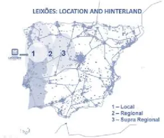
The hinterland of the Port of Leixões corresponds to its area of influence on land. APDL divides its hinterland into local, regional and supra regional, as depicted in Figure 1.
On the other hand, the foreland is the set of final destinations reached, via connected ports, which, in the case of the Port of Leixões, corresponds to 184 countries. Note that this information about the foreland is provided by the concessionaires since the evidence that APDL has is not accurate.
2.3 Previous studies
According to UNCTAD (1993, p. 3): “Of the various reasons for collecting data relating to ports, two are of primary concern to port authorities: first, the data can be used for improving port operations, and secondly, they can provide an appropriate basis for planning future port development.”
Most of the previous studies focus on internal factors to assess the performance of ports, and very few on external factors. Nevertheless, our study focuses on external factors that may influence cargo movements in ports.
• Hinterland and competition
Understanding the concept of hinterland is crucial when it comes to ports. Ports hinterlands correspond to the geographical area that a port or terminal serve (Carvalho et al., 2015), i.e., the area covered by all the companies that use the port. Therefore, geography defines the port a company uses, and competitive markets are often caractherized by the ports that share the same hinterlands.
Meersman et al. (2010, p. 218) claim that the issue that must be addressed is “competition between supply chains”, of which ports are part, and the crucial aspect to consider is the cost of these chains. Langen (2007) corroborates this idea, defending a paradigm shift in which one must consider that ports do not provide an isolated service, but rather a service that is included in a supply chain.
Therefore, according to Meersman et al. (2010), when the hinterlands coincide, the choice between ports will be based on the port that contributes to a lower cost supply chain. Consequently, the question that should be asked by the port user is: “does the port considered offer advantages compared to other ports serving the same hinterland?” (Meersman et al., 2010, p. 219).
Moreover, Langen (2007) studied the case of Austria, which constitutes the hinterland of 6 different European ports. This author demonstrated that the market share of the different ports varied over time, which corroborates the idea of competition between ports within the same geographical area.
Accordingly, cargo movements of a given port depend, not only on the conditions of this port, but also on the conditions that other ports, that have the same hinterland, offer to potential port users.
• Climate
The Committee on Climate Change, US Transportation, Transportation Research Board, Division on Earth, & Life Studies (2008) identifies both positive and negative impacts of climate in ports. For instance, a positive impact of an abnormal climate event is the impediment of accumulation of ice on ships by the existence of warmer winter days.
According to the same report, ports infrastructures are constructed taking into account the possibility of adverse weather conditions. Nevertheless, extreme situations may “push environmental conditions outside the range for which the system was designed.” (p. 49). Therefore, it is important to acknowledge that climate can affect the movements of cargo since it can disturb the security, normal operation of ports and maintenance of the infrastructures and systems.
It should be noted that maritime transport systems, i.e., seaports, are located in coastal areas which are very vulnerable, for instance, to storms or sea-level rise. (Becker et al., 2011)
• Other transportation modes
International trade consists of the exchange of goods and services between countries, allowing the sharing of new products and experiences around the world. Maritime transport is one of several modes of transport used in international trade.
Thus, maritime transport is inherently linked to international trade. In an increasingly globalized economy, in which countries are highly dependent on each other, either because of international trade or investment, ports assume importance in fostering trade (Blonigen & Wilson, 2008).
Sánchez et al. (2003) claim that improvements in the means of transport at international level promote economic globalization. According to these authors, a reduction in transport costs leads, directly, to a stimulus of imports and exports.
In the publications of INE5 and PORDATA6, in the main statistical results on the activity of the Transport and Communications sectors in Portugal, it is possible to observe the statistics on international trade by mode of transport. As far as imports and exports are concerned, maritime transport is the mode of transport responsible for the majority of the volume of goods imported in recent years. In 2017, maritime transport accounted for 61.6% of the volume of imported goods, which corresponds to 39.2 million tons, and 54.6% of the volume of exported goods. However, the value of each ton imported and exported is lower when the transport is done by sea than road, so the
5 https://www.ine.pt/xportal/xmain?xpgid=ine_main&xpid=INE 6 https://www.pordata.pt/
percentage of this mode of transport on imports and exports in euros is lower than the road. Thus, in 2017, maritime transport represented 26.1% and 30.8% of imports and exports in value, while road transport represented 61.9% and 60.5%, respectively.
Chapter 3
Methods
This chapter introduces the analytical method used in our empirical analysis, which is regression analysis. This is a predictive analytics method, as pointed out in chapter 1. There are various predictive models. Our choice for regression methods is due to the fact that regression analysis is the most established method for predicting continuous variables, allowing to extract insights from data, specially about the relation between predictive and explanatory variables. In the case of our study, we have one dependent continuous variable and several explanatory variables, some of which are categorical and others quantitative. Thus, among the most appropriate analyses, we decided to adopt multiple regression.
We divided this chapter in two parts, one dealing with the methods require to pre-process the data and the second part where the regression analysis is presented.
3.1 Pre-processing data
After the problem has been formulated and the data collected, there is some steps to be taken, namely:
i. organizing the data into an appropriate format to entry them in the software, R in our case;
ii. data preparation.
These steps are crucial to make the data suitable for analysis and to produce more effective results.
to the variables and the rows correspond to the observations, as shown by Figure 2.
Figure 2:Matrix representation
Secondly, the data preparation phase must be completed before starting the analysis.
In the real world, the data that are collected are not perfect, data are often inconsistent, with outliers and missing values that make it noisy and incomplete.
According to Soibelman and Kim (2002), data preparation is the hardest and most time-consuming phase of the statistic process. Next, there is an explanation of how to handle these types of problems, through data preparation, according to the same authors.
Firstly, data cleaning consists of improving the quality of the data by solving problems, such as missing data, noisy data, outliers and contradictions.
There are several ways to deal with missing data, such as ignore the records or the attributes that include them. However, these solutions may lead to insufficient sample sizes or the elimination of important variables. Furthermore, other ways to deal with this problem is to use the most probable value, or a global constant, such as “unknown”, or the mean or median of that attribute to fill the missing value.
When it comes to atypical observations, outliers, there are more than a few methods to deal with these: binning method, which divides the data into bins and then smooth it by bins mean, medians or others; regression, by fitting the
data into regression functions; classical statistical method, by detecting outliers with, for instance, boxplots, and then removing them; clustering, by detecting and removing outliers; combined computer and human inspection.
Secondly, data integration consists in merging data from different sources in order to give the user a unified view of these data. It is important, when doing this step, to take into account that data value conflicts and redundancy problems can happen.
Thirdly, data transformation involves processes such as generalization, the possible construction of new features from old ones and the normalization of data.
Fourthly, data reduction involves the sampling of data, selecting of features, and reduction of the dimension of the data. In this step of data preparation, it can be selected a subset of objects or variables to be analysed, or new features can be created from the old ones. It is important that the information available in the new, reduced, dataset is a good representation of the original information.
Lastly, data discretization is the process of converting continuous-valued attributes into discrete variables with a small number of values.
Therefore, the data is ready, and the statistical analysis can begin. “When data are properly prepared, the analyst gains understanding and insight into the content, range of applicability, and limits of data” (Soibelman et al., 2002, p. 42).
3.2 Regression
A regression model is used to explain the relationship between a dependent variable, Y, and a set of explanatory variables, 𝑋1, 𝑋2, ..., 𝑋k.
𝑋2, ..., 𝑋k are the explanatory variables and ε is a random perturbation/
disturbance.
The regression coefficients are constant, and each 𝛽𝑘 represents the expected
variation in Y when 𝑋k increases one unit and the other variables remain
constant. However, in linearized models, i.e., where there are logarithmic transformations, for the dependent and independent variables, then 𝛽𝑘
represents the expected percentage change in Y when 𝑋𝑘 increases by one
percentage point and the other variables remain constant.
The random disturbance is the way of the model to take into account the randomness of choice of the model variables, as a human action. Therefore, ε disturbs and neutralizes the exact measurement of the explained variable.
The literature is unanimous regarding the idea that the initial data analysis, before estimating the models, should consist in making summary and descriptive statistics of the variables. Faraway (2009) states that, in this phase, it is important to be aware and seek for uncommon or surprising values. Additionally, histograms and boxplots can be constructed in the sense of perceiving the distribution of each of the variables individually, or scatterplots and dynamic charts to relate two or more variables.
After estimating the parameters of the model, the statistical significance of each of the explanatory variables must be analysed, in order to understand how these influence the dependent variable. Similarly, the overall measure of the quality of the adjustment, the coefficient of determination (R2), must also be considered. The R2 explains which percentage of the dependent variable is explained by the model.
Furthermore, many authors consider a set of key assumptions underlying regression analysis that must be verified for the inferences drawn to be accepted: multicollinearity, homoscedasticity and autocorrelation.
Multicollinearity occurs when the variables of the model are linearly associated. The diagnosis of the presence of multicollinearity can be performed through the analysis of the correlations between the variables and, formally, through the analysis of the values of Generalized Variance Influence Factors (GVIF) (Fox & Monette, 1992), which when high are indicators of multicollinearity.
The heteroscedasticity is a problem to be taken into consideration, since, in existence, it violates one of the assumptions of the least squares method, that: var (yi) = var (ei) = σ2, negatively affecting estimation and inference statistic.
This can be diagnosed graphically, using residual plots, or formally, through the Breusch-Pagan test. This test has, as null hypothesis, the presence of homoscedasticity, i.e., conditional variance is constant, against the opposite alternative, heteroscedasticity, i.e., the disturbances do not have the same variance.
When heteroscedasticity is suggested, the way to continue the regression analysis in its presence is by using robust standard errors, suggested by Halbert White. This does not eliminate heteroscedasticity, but rather enables the usual techniques of statistical inference from the results of the adjustment.
Moreover, comparing the standard errors with the robust standard errors that emerged from the "remedy" applied to heteroscedasticity, the results must be analysed to see if they changed or not.
Autocorrelation happens when disturbances are dependent over time. This assumption can be verified graphically by analysing the graph with the residuals as a function of the estimated values of the dependent variable, and if a pattern is identified, it suggests the presence of autocorrelation. To test this assumption formally, the Durbin-Watson test can be performed, whose null hypothesis states that the residuals are not correlated.
To continue the estimation in the presence of autocorrelation, a heteroscedasticity and autocorrelation consistent covariance matrix, proposed by Andrews (1991), can be used. Hence, with this method, the tests of significance of the parameters are done with robust standard errors that are valid. As in the case of the remedy applied to heteroscedasticity, the results of the estimation should be compared to see if the conclusions change.
Some authors also add the assumption of normality for inference in small samples. This assumption states that the disturbances follow a normal distribution with a null mean. This assumption can be verified graphically, where, if the data are symmetrical and the points follow the straight line, the residuals follow a normal distribution. It should be noted that regression does not require this assumption, since, according to Eicker (1963) and Weisberg (2005), when the samples are large, many tests become valid.
However, when the disturbances are not normally distributed, outliers may be more common, so a proper analysis of outlier influence should be conducted. To understand if there are severe outliers, the Bonferroni Test can be performed, whose null hypothesis refers to their absence. Furthermore, if the test suggests the presence of severe atypical observations, one can identify which outliers are most influential through the analysis of the hat values, graphically. Subsequently, the model is estimated excluding these observations, in order to verify if the results change.
Chapter 4
Data and Sample
As previously stated in Chapter 1, the goal of this study is to explain the tonnage of cargo moved in the port of Leixões from 2009 until 2017. The variables used in our analysis are shown in Table 1. It should be noted that there were more variables available than those used, but in the final models they were not relevant, so we omit them for sake of simplicity.
Table 1: Variables
Variables Description Classification
Leixões Tonnage Year Month Cargo Type Lisbon Tonnage Sines Tonnage Aveiro Tonnage Quarterly GDP Strikes
Tonnage moved in the port of Leixões Year of the movement: from 2009 to 2017
Number of the month of the movement: from 1 to 12 Classification of the cargo: Containers; Liquid bulk; Others Tonnage moved in the port of Lisbon
Tonnage moved in the port of Sines Tonnage moved in the port of Aveiro
Value of the quarterly GDP, in millions of euros Strikes in that month: 0- No; 1- Yes
Quantitative Quantitative Categorical Categorical Quantitative Quantitative Quantitative Quantitative Categorical
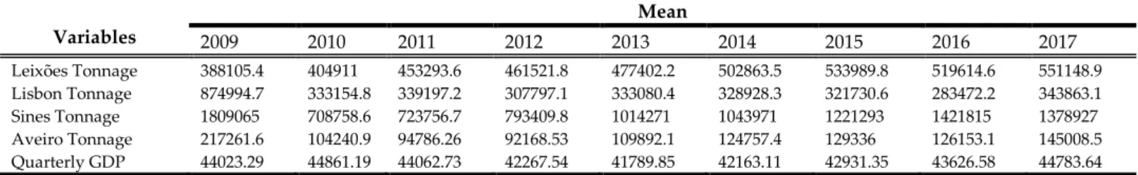
Tables 2 and 4 show the descriptive statistics of the quantitative and categorical variables, respectively.
Table 2: Descriptive statistics of the quantitative variables: mean per year
Variables Mean 2009 2010 2011 2012 2013 2014 2015 2016 2017 Leixões Tonnage Lisbon Tonnage Sines Tonnage Aveiro Tonnage Quarterly GDP 388105.4 874994.7 1809065 217261.6 44023.29 404911 333154.8 708758.6 104240.9 44861.19 453293.6 339197.2 723756.7 94786.26 44062.73 461521.8 307797.1 793409.8 92168.53 42267.54 477402.2 333080.4 1014271 109892.1 41789.85 502863.5 328928.3 1043971 124757.4 42163.11 533989.8 321730.6 1221293 129336 42931.35 519614.6 283472.2 1421815 126153.1 43626.58 551148.9 343863.1 1378927 145008.5 44783.64
The tonnage of cargo moved in the port the Leixões is our dependent variable. The dataset contained 31627 cargo movements of embarkation and
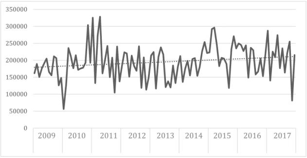
September of 2018. The graph of Figure 3 depicts the values in table 2 and shows the increasing trend in the cargo movements in the port of Leixões in tons, from 2009 to 2017.
Figure 3: Leixões Tonnage
In each year of the series there are monthly fluctuations of the tons of cargo handled. However, these monthly oscillations are not regular throughout the series, i.e., there is no seasonality. This is found when comparing the cargo of each month with the average of the cargo of the corresponding year.
For example, in 2014, December has a higher than average cargo movement, being the month with the highest cargo movement in that year, while, in the previous year, its tonnage movements are below the average, being the month with the least cargo handling in 2013.
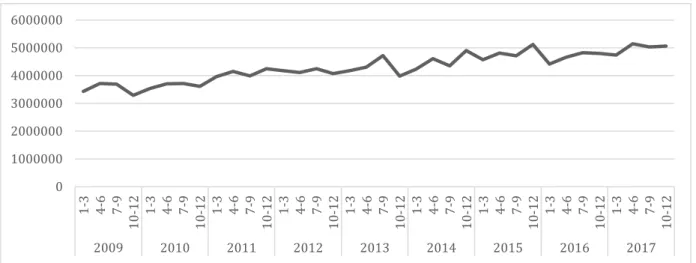
After grouping the data by quarter, in the graph of Figure 4, the monthly cargo movements are presented quarterly.
0 500000 1000000 1500000 2000000 2500000 2009 2010 2011 2012 2013 2014 2015 2016 2017
Figure 4: Total tonnage per quarter
When the analysis is done by quarter, it is still observed the trend of growth starting from 2011. It can also be noted that: starting in 2014, the quarter with the lowest amount of cargo handled is always the first; in 2014, 2015 and 2016, the quarter with the highest cargo handling is the last; there are oscillations, but these are not regular throughout the series.
Furthermore, APDL considered that competing ports were mainly those located in the geographical proximity and overlap of hinterlands of the port of Leixões.
It is important to note that the ports are monopolistic in most of its concessions, since operations involve investments in infrastructures of high economic value. Consequently, APDL explained that only in situations of suspending operations, which involve the diversion of cargo to another port, it is clear who is the competition.
As for data from other ports, the tons of cargo handled in the ports of Lisbon, Sines and Aveiro are considered explanatory variables. APDL identified its competitors, by type of cargo, as presented in Table 3.
0 1000000 2000000 3000000 4000000 5000000 6000000 1-3 4-6 7-9 10 -1 2 1-3 4-6 7-9 10 -1 2 1-3 4-6 7-9 10 -1 2 1-3 4-6 7-9 10 -1 2 1-3 4-6 7-9 10 -1 2 1-3 4-6 7-9 10 -1 2 1-3 4-6 7-9 10 -1 2 1-3 4-6 7-9 10 -1 2 1-3 4-6 7-9 10 -1 2 2009 2010 2011 2012 2013 2014 2015 2016 2017
Table 3: Competitors by type of cargo
Cargo Type Competitors
Containerized cargo Liquid Bulk cargo Break Bulk cargo Ro-Ro cargo Dry Bulk cargo
Lisbon, Sines, Vigo and Setúbal Sines and Coruña
*
Setúbal and Vigo Aveiro
* information not provided
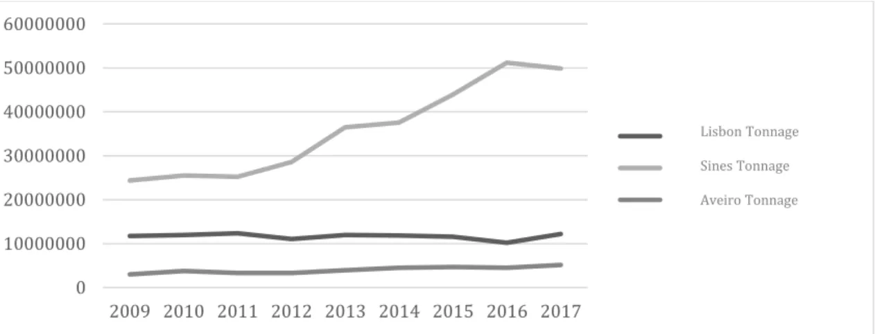
The evolution of these cargo variables in the other ports throughout the time series is shown in Figure 5 (where we only show annual values).
Figure 5: Other ports cargo
The evolution of the tonnage of cargo handled in the relevant ports, identified by APDL as its competitors, is stable, except in the port of Lisbon. Unlike the rest, the port of Lisbon has a higher amount of cargo moved over the years and a growing trend from 2011.
The last variable in Table 2 is GDP. This variable is calculated at market prices from the perspective of the expenditure and was obtained from the Quarterly National Accounts (“Contas Nacionais Trimestrais”) published by INE in the first trimester of 2018.
This choice of variable is justified by two reasons, according to the APDL: firstly, about 80% of the final customers are located in the metropolitan area of
0 10000000 20000000 30000000 40000000 50000000 60000000 2009 2010 2011 2012 2013 2014 2015 2016 2017 Soma de Tonnage_LISBON Soma de Tonnage _SINES Soma de Tonnage_AVEIRO
Lisbon Tonnage Sines Tonnage Aveiro Tonnage
Porto, Portugal; secondly, according to the company, it is expected that the movements in the port of Leixões are a reflection of the economic activity of the context where it is inserted. Thus, the industrial dynamics of the Portuguese region could determine the functioning of the port.
It should be noted that, although there is no access to data regarding the main customers of APDL, it is known that one of its main customers is GALP, which is a Portuguese company that operates in the oil terminal using the “monoboia”, whose head office is in Porto. Another major client is “Sidurgia da Maia” that imports scrap and exports iron and steel, whose location, as the name implies, is in Maia, Portugal.
The evolution of the quarterly GDP throughout the time series studied is shown in Figure 6.
Figure 6: Quarterly GDP of Portugal
The quarterly GDP grows until the third quarter of 2010, when it reaches a high peak. From then on, it falls until the third quarter of 2012, when it assumes a growth trend until the end of the time series.
350000 360000 370000 380000 390000 400000 410000 1-3 4-6 7-9 10 -1 2 1-3 4-6 7-9 10 -1 2 1-3 4-6 7-9 10 -1 2 1-3 4-6 7-9 10 -1 2 1-3 4-6 7-9 10 -1 2 1-3 4-6 7-9 10 -1 2 1-3 4-6 7-9 10 -1 2 1-3 4-6 7-9 10 -1 2 1-3 4-6 7-9 10 -1 2 2009 2010 2011 2012 2013 2014 2015 2016 2017
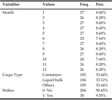
Table 4 shows the descriptive statistics of the categorical variables used.
Table 4: Descriptive statistics of the categorical variables
Variables Values Freq. Perc.
Month Cargo Type Strikes 1 2 3 4 5 6 7 8 9 10 11 12 Containers Liquid bulk Others 0- No 1- Yes 27 26 27 27 27 24 27 26 27 24 26 26 105 104 105 284 30 8.60% 8.28% 8.60% 8.60% 8.60% 7.64% 8.60% 8.28% 8.60% 7.64% 8.28% 8.28% 33.44% 33.12% 33.44% 90.45% 9.55%
Three segments of cargo were considered in our analysis: containers, liquid bulk cargo and others.
Originally, APDL classifies them into 5 categories: containerized cargo, liquid bulk cargo, break bulk cargo, roll-on roll-off (Ro-Ro) cargo and dry bulk cargo. We reduced the number of categories, by creating the type of cargo “others” that includes the remaining 3 categories mentioned above.
Each type of cargo has its own requirements, implying an adequate infrastructure. For instance, the Ro-Ro cargo corresponds to the cargo entering and leaving the ship by means such as wheels and ramps, no cranes required. This type of cargo is moved in the Ro-Ro Terminal. Furthermore, in the oil terminal, the oceanic “monoboia” allows to move oil that belongs to the liquid bulk cargo type.
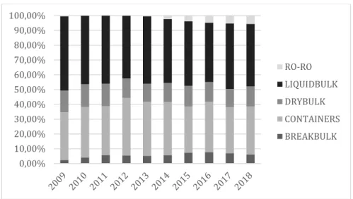
The two types of cargo that are mostly handled in the port of Leixões are liquid bulk and containerized cargo, as shown by Figure 7. The Ro-Ro cargo,
despite having a small proportion of the global movements in the port of Leixões, has been increasing since 2013.
Figure 7: Percentage of each type of cargo moved per year
In addition, we made an analysis of the evolution of the tonnage moved in port of Leixões per type of cargo, namely: containerized cargo (Figure 8), liquid bulk cargo (Figure 9), RO-RO cargo (Figure 10), breakbulk cargo (Figure 11) and dry bulk cargo (Figure 12).
0,00% 10,00% 20,00% 30,00% 40,00% 50,00% 60,00% 70,00% 80,00% 90,00% 100,00% RO-RO LIQUIDBULK DRYBULK CONTAINERS BREAKBULK 0 100000 200000 300000 400000 500000 600000 700000 800000 2009 2010 2011 2012 2013 2014 2015 2016 2017
When one observes the evolution of the tons of containerized cargo moved, in Figure 8, there is a clear trend of growth from 2009 to 2014. At the end of 2014 and the beginning of 2015, there is a drop, but the trend of growth continues to occur.
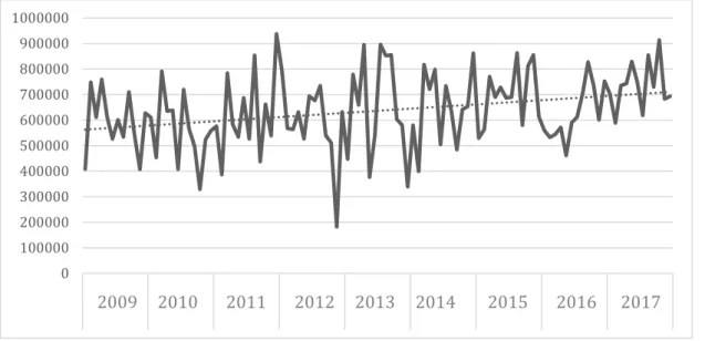
Figure 9: Liquid bulk cargo tonnage per month
As for liquid bulk, there is evidence of marked oscillations throughout the time series, as it is clear in Figure 9. In the case of this type of cargo, regular oscillations are observed throughout the series: in the years from 2009 to 2013, except in 2011, the lowest peaks of movements of cargo were at the end of the year, whereas, in the years from 2014 to 2017, these peaks were at the beginning of the year. However, there does not seem to be a pattern in the peaks of higher cargo handling. 0 100000 200000 300000 400000 500000 600000 700000 800000 900000 1000000 2009 2010 2011 2012 2013 2014 2015 2016 2017
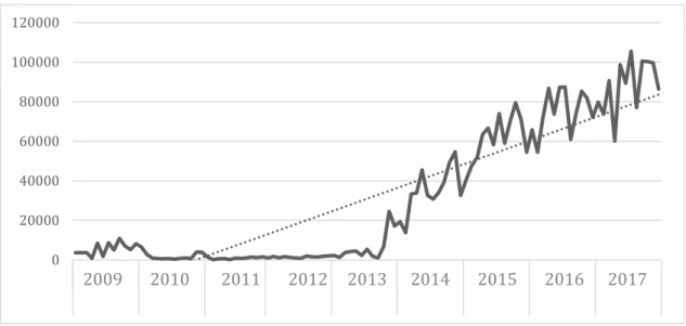
Figure 10: RO-RO cargo tonnage per month
RO-RO cargo movements, although very low at the beginning of the time series, show a strong growth trend from 2013, as depicted in Figure 10.
Figure 11: Breakbulk cargo tonnage per month
Figure 11 shows that the evolution of breakbulk cargo movements has a growth trend, although it has a lot of oscillations. However, it has a decrease
0 20000 40000 60000 80000 100000 120000 2009 2010 2011 2012 2013 2014 2015 2016 2017 0 20000 40000 60000 80000 100000 120000 140000 160000 180000 2009 2010 2011 2012 2013 2014 2015 2016 2017
Figure 12: Dry bulk cargo tonnage per month
As for dry bulk cargo, its movements are characterized with a lot of oscillations. It can be observed an extreme low peak in 2009 and 2017, and a high peak in 2011.
Furthermore, in order to include strikes as a variable, a binary explanatory variable was created, where 0 corresponds to the months of normal workflow of all ports operations and 1 corresponds to the months where there was at least one strike in one Portuguese port.
The data regarding strikes was collected through the internet, namely, news sites.
There are several situations that lead to the paralysis of port operations, specifically strikes and construction work.
Strikes are a way for employees to negotiate working conditions. According to the Constitution of the Portuguese Republic (Constituição da República Portuguesa, Artigo 57º), workers in Portugal have the right to strike, i.e., the right to voluntarily and collectively suspend the performance of their work in order to achieve a certain goal related to their jobs.
0 50000 100000 150000 200000 250000 300000 350000 2009 2010 2011 2012 2013 2014 2015 2016 2017
Strikes and port operation stoppages can lead to the change of the scale of ships, diverting cargo to other ports. Thus, these events can have an impact on the cargo movements in the ports.
An extended stoppage may be favorable for the port of Leixões, when it occurs in ports and leads to a diversion of cargo to Leixões, increasing its cargo movements, or unfavorable if it occurs in Leixões, decreasing its cargo movements. For instance, a stop of 3 or more weeks at the Sines refinery is quite favorable to the port of Leixões, as it is its competitor at liquid bulk cargo level. Therefore, these cargoes will be diverted to the refinery of Leixões, implying an increase in the cargo movements of Leixões.
4.1 Non-included variables
There were other explanatory variables that we would like to have tested but were not possible to collect, or that we tested, but which were not included in the final models.
Climate, measured through weather conditions like rain, sea agiation, etc.., was one possible explanatory variable suggested to be used in the analysis of the monthly movements of cargo in the port of Leixões, given that the weather conditions have impacts on transportation. However, collaborators at the Port Authority argue that in the port of Leixões there is no climate effects on the movement of cargo in the long term, only in the short term. For instance, if there is a storm that prevents a ship from entering the port to unload or upload cargo, it waits until it is possible to enter. According to the APDL, there has never been a diversion of cargo to another port, or vice versa, due to bad weather or an abnormal climate event. Another example is the tide. When there is strong sea agitation, it is not possible to operate the “monoboia”, so the activities in it are suspended. However, the refinery is already waiting for these
episodes, so they are compensated in other periods. Therefore, we did not test for climate related variables.
Nevertheless, we created an explanatory binary variable that distinguishes summer and winter months, such that we can analyse seasonality, which is, for obvious reasons, related to climate. Specifically, the pattern of seasonality that we considered was to distinguish between summer and winter months. However, this was not a statically significant variable. Note that the month was considered in our models, so in a sense we still accommodate for some seasonal effects.
The “other modes of transport” was an explanatory variable that we would like to have tested. The modes of transportation may be complementary as well as competitors of the maritime transport of the port of Leixões. Since there is no way to distinguish the two from the available data, we could conclude, by its major effects on the movement, if the majority of the other transportation modes are complementary or rival. For instance, on the one hand, a cargo can be transported to Rotterdam by ship or by road transport mode, in which case they are competing modes of transport. On the other hand, if a cargo arrives at the port of Leixões with final destination in a Vila Real company, it will have to be transported from the port to the company by road or rail, so in this case they are complementary modes of transport. Ideally, we would like to have available data regarding other transportation modes, but it was not possible to collect those data.
In addition to the variables mentioned, we also created a variable, “Time”, in order to analyse the effect of the evolution throughout the time. This variable indexes the months considered, from 1 (January 2009) to 108 (December 2017). This variable was not statistically significant as well.
Chapter 5
Data analysis
Two different studies were developed: the first one aims to explain the total tonnage of cargo moved in the port of Leixões, while the second tried to perceive the same, but by type of cargo.
We started by preparing the dataset.
5.1 Dataset
To carry out the study, a database containing 314 observations and 14 variables was constructed.
The first phase consisted of data pre-processing.
First, we started by verifying and correcting the classification of all the variables. Moreover, the original data included some negative tonnage values in the variables about the other ports. This is due to the fact that the other ports do not consider the same classifications for the cargo as APDL, so this company has to estimate the tonnage for each type of cargo from those data, and sometimes there are errors that result from the automatic way of calculation. Therefore, we thought it was best to erase the observations that contained negative tonnage. This choice is justified by the number of observations erased, 10, which is relatively small, since the original sample had 324 observations.
Also, we found that the number of missing values in each row of the dataset was zero.
As for data reduction, for the purpose of the subsequent analysis, we created three subsets for each type of cargo: “containers”, “liquidbulk” and “others”.
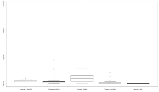
Figure 13: Boxplots of the quantitative variables
Thus, it is clear the existence of atypical values, i.e., atypical cargo movements in some months, in the ports of Leixões, Lisbon, Sines and Aveiro. Later, when studying each model, we discovered if there were severe outliers and, if so, if they were influential.
5.2 Regression model: Leixões Tonnage
As previously stated, in the context of our study, we developed a regression model that helped us to explain the movements of cargo in Leixões.
Before arriving at the final model, we estimated several models.
Firstly, we noticed that the time related variables, “month”, “time” and “seasonality” had a perfect linear relationship, originating multicollinearity, so we started by estimating three different models, including in turn one of these variables.
We estimated numerous models, until we got simpler and reduced models, with most explanatory variable coefficients as statistically significant.
We followed a general to specific strategy to search for an appropriate model, using the Akaike Information Criterion (AIC) as a guiding principle. We tested this model against a full model with all non colinear possible explanatory variable by an ANOVA F test, accepting the validity of our chosen model.
Then, we studied the effect of interactions between the tonnage of cargo handled in Sines and the existence or absence of strikes. The hypothesis that arises in this case is that the existence of strikes can lead to the diversion of cargo from one port to another.
The use of interaction terms implied the need to centre our Sines Tonnage variable to facilitate the interpretation of the coefficients.
The model with the interactions explained the cargo movements of Leixões in a larger percentage, i.e., had a larger R2 than the model without it, which means that the interactions contribute to explain the movements in Leixões.
Table 5: Regression model RegAI
RegAI
Estimate Std. error t P-value
Intercept -4.452e+07 4.191e+06
2.082e+03 2.485e+04 2.461e+04 2.469e+04 2.460e+04 2.548e+04 2.478e+04 2.493e+04 2.468e+04 2.542e+04 2.528e+04 2.492e+04 1.325e+04 1.289e+04 1.801e+04 5.402e-03 2.683e-02 -10.622 10.731 -1.171 2.675 2.463 1.390 0.918 2.416 1.913 0.510 1.937 0.828 1.626 12.008 -14.711 -2.330 -1.817 -3.310 0.00 *** Year Month 2 (ref:January) Month 3 (ref:January) Month 4 (ref:January) Month 5 (ref:January) Month 6 (ref:January) Month 7 (ref:January) Month 8 (ref:January) Month 9 (ref:January) Month 10 (ref:January) Month 11(ref:January) Month 12 (ref:January)
Cargo Type Liquid bulk (ref: Containers) Cargo Type Others (ref: Containers) Strikes (ref: No)
Sines Tonnage
Sines Tonnage * Strikes
2.234e+04 -2.909e+04 6.583e+04 6.082e+04 3.419e+04 2.340e+04 5.987e+04 4.771e+04 1.257e+04 4.923e+04 2.093e+04 4.051e+04 1.592e+05 -1.896e+05 -4.197e+04 -9.817e-03 -8.879e-02 0.00 *** 0.24273 0.00789 ** 0.01434 * 0.16563 0.35922 0.01630 * 0.05667 . 0.61075 0.05373 . 0.40843 0.10508 0.00 *** 0.00 *** 0.02045 * 0.07018 . 0.00105 ** R2 73.58%
Note: significance level at 0.1% (***), 1% (**), 5% (*) and 10%(.)
The p-value of the F test of this model is very close to zero, which testifies the statistical significance of the model and the importance of the explanatory variables in explaining the Tonnage of Leixões.
Making a more concrete analysis of the impact that the chosen variables have, we can draw the following conclusions:
• In the estimated model the cargo movements in the Port of Leixões are explained in about 73.58%;
• There is a growth trend over the years;
• Although there are no statistically significant effects in most of the months, March, April and July are typically the months when more cargo movements are expected, compared to January;
• There is likely to be less movement of “others” cargo and more movement of liquid bulk cargo than of the reference type, containers;
• There is likely to be less movement of cargo in Leixões when there are strikes, compared to when there are no strikes, when Sines Tonnage is equal to its sample average;
• An increase of 1 kilogram of cargo moved in the port of Sines leads to a reduction of, approximately, 10 kilograms (9.82) in the port of Leixões, when there are no strikes;
• When there are strikes, the reduction of tons moved in Leixões, caused by each additional ton of Sines, increases by 9 kilograms, that is, it decreases by 19 kilograms, compared to when there are no strikes.
5.2.1 Assumptions
• Multicollinearity
To determine if the variables were linearly associated, we analysed the correlation between the numeric variables, and it was not strong.
In order to formally diagnose the presence of multicollinearity, we analysed the values of GVIF, which when high are indicators of multicollinearity. The higher GVIF was 1.19, which is not substantial. So, we did not detect multicollinearity.
• Heteroscedasticity
In order to determine if the model was heteroscedastic or homoscedastic, i.e., if the variance of "Tonnage_Leixoes" depended on the observations or not, we proceeded to the diagnosis. Firstly, we analysed the graphical representations, present in Figure 14.
Figure 14: Residual Plots
The graphs suggest the presence of heteroscedasticity, namely through three fonts: first, the residuals vary more when the type of cargo is liquid bulk; second, a greater variability of the residuals is observed in the autumn/winter months; finally, although the scale is not ideal, the residuals vary more when the tonnage moved in the port of Sines is higher.
In order to formally test the evidence for heteroscedasticity, we performed the Breusch-Pagan test. The p-value was very close to zero, so we can reject the null hypothesis.
Furthermore, in order to proceed with our analysis with the presence of heteroscedasticity, not to eliminate it, but to enable the usual techniques of statistical inference from the results of the adjustment, we proceeded to test the robust standard errors, suggested by Halbert White. Comparing the standard errors with the robust standard errors that emerged from the "remedy" applied to heteroscedasticity, we found that the results did not change significantly.
• Autocorrelation
Since we have 3 observations for each month, corresponding to each type of cargo, in order to verify the presence or absence of autocorrelation, we had to do the test proposed by Wooldridge (2002) for panel data.
The test detected autocorrection. One of the common measures to deal with autocorrelated residuals would be to use robust standard errors, such as those proposed by Arellano (1987). However, the best-known variant of these errors relies on large n asymptotic (where n is the number of cases by time unit) and is not applicable in our setting, where n is only equal to 3.
Therefore, in the future, these problems should be taken into account.
• Normality
The assumption of normality accepts that the residuals follow a normal distribution with a null mean. To verify the normality of the data, we analysed the graph of Figure 15.
Figure 15: Normality of the model RegA
on asymptotic arguments to perform the analyses in the absence of normally distributed disturbances (Eicker, 1963 and Weisberg, 2005). Nevertheless, afterwards we performed an influence analysis to check possible negative effects of large outliers.
5.2.2 Outliers Analysis
To understand if the atypical observations, identified in section 5.1, skewed the chosen model, we started by identifying the severe outliers. The Bonferroni Outlier Test suggested that there were observations that were severe outliers. The graphs of Figures 16 and 17 allowed us to make the diagnosis of the influential outliers, given by observations 107, 140 and 265.
Figure 17: Influence measures
We estimated the model without the influent outliers and the conclusions did not change.
To sum up, the regression analysis allowed us to identify the main external determinants of the cargo movements in the port of Leixões: year of movement, month of movement, type of cargo, tonnage moved in the port of Sines, existence or absence of strikes and interaction between the Sines tonnage and the binary variable of the strikes.
It makes sense that the cargo movements in the port of Sines influences those in the port of Leixões, since this port was identified by APDL as one of the main competitors, namely in terms of the busiest cargoes, containers and liquid bulk.
As for the interaction, the fact that it is statistically significant to explain the cargo movements in the port of Leixões shows that the shift of cargo between Leixões and Sines during the strikes is significant. In this case, the existence of strikes causes a reduction of the tons in Leixões that is greater with the increase of the cargo moved in Sines, that is, the strikes lead to a diversion of cargo in
5.3 Regression Models: per type of cargo
Additionally, we decided to understand the main external determinants of the movements of each type of cargo in the port of Leixões. Accordingly, as mentioned earlier, in the data reduction phase, we created 3 subsets for each type of cargo: containerized, liquid bulk and others.
Note that the processes were very similar to the processes described in the previous section.
5.3.1 Containerized cargo
In order to answer the research question for the containerized cargo, we started by estimating several models, until we had the final one. This model has the largest determination coefficient (R2) and its explanatory variables are all statically significant.
The estimation of this model is in table 6.
Table 6: Regression model Reg1C_step
Reg1C_step
Estimate Std. error t P-value
Intercept -2.672e+07 1.407e+04 -1.748e+04 4.917e+04 2.190e+04 5.474e+04 4.763e+04 6.546e+04 3.296e+04 2.948e+04 8.842e+04 9.447e+04 4.650e+04 -1.906e-02 -1.167e+02 -2.643e+01 3.549e+04 2.884e+06 1.426e+03 1.648e+04 1.649e+04 1.654e+04 1.649e+04 1.711e+04 1.674e+04 1.656e+04 1.649e+04 1.707e+04 1.813e+04 1.656e+04 7.915e-03 4.030e+01 3.026e+00 1.213e+04 -9.266 9.869 -1.061 2.982 1.324 3.320 2.784 3.910 1.990 1.788 5.179 5.210 2.809 -2.409 -2.895 -8.735 2.925 1.16e-14 *** 6.69e-16 *** 0.291690 0.003703 ** 0.188981 0.001310 ** 0.006569 ** 0.000181 *** 0.049655 * 0.077181 . 1.40e-06 *** 1.23e-06 *** 0.006130 ** 0.018092 * 0.004779 ** 1.44e-13 *** 0.004378 ** Year Month 2 (ref:January) Month 3 (ref:January) Month 4 (ref:January) Month 5 (ref:January) Month 6 (ref:January) Month 7 (ref:January) Month 8 (ref:January) Month 9 (ref:January) Month 10 (ref:January) Month 11(ref:January) Month 12 (ref:January) Lisbon Tonnage Aveiro Tonnage Quarterly GDP Strikes (ref: No)
R2 78.74%
Interpreting the coefficients of the explanatory variables of the estimated model, it is possible to conclude:
• In the estimated model the containerized cargo movements in the port of Leixões are explained in about 78.74%;
• There is a growth trend over the years;
• In most of the months, except February, it is expected more cargo movements than in January;
• An increase of 1 kilogram of containerized cargo moved in the port of Lisbon leads to a reduction of 19 kilograms in the port of Leixões; • An increase of 1 kilogram of containerized cargo moved in the port of
Aveiro leads to a reduction of 11.7 kilograms in the port of Leixões; • An increase of 1 million euros in the quarterly GDP leads to a
reduction of, approximately, 26 kilograms of conteinerized cargo in the port of Leixões;
• There is likely to be more movement of containers in Leixões when there are strikes, compared to when there are no strikes.
5.3.1.1 Assumptions
• Multicollinearity
The numerical variables do not have a very strong correlation with each other. However, there is a positive correlation above 0.5 between the variables Lisbon Tonnage and Aveiro Tonnage (0.51). Thus, the correlation between the tons of containerized cargo moved in Lisbon and those moved in Aveiro suggests that an increase in one kilo of cargo in the port of Lisbon will lead to an estimated increase in the cargo handled in Aveiro of 0.51 kilograms.