A decision support system in shuttle service managing

Universidade de ´

Evora - Escola de Ciˆ

encias e Tecnologia

Mestrado em Engenharia Inform´atica

Disserta¸c˜ao

A decision support system in shuttle services managing

Jo˜ao Pedro Candeias Coxinho Tom´e Aldeano

Universidade de ´

Evora - Escola de Ciˆ

encias e Tecnologia

Mestrado em Engenharia Inform´atica

Disserta¸c˜ao

A decision support system in shuttle services managing

Jo˜ao Pedro Candeias Coxinho Tom´e Aldeano

A disserta¸c˜ao foi objeto de aprecia¸c˜ao e discuss˜ao p´ublica pelo seguinte j´uri nomeado pelo Diretor da Escola de Ciˆencias e Tecnologia:

Presidente _{| L´ıgia Maria Rodrigues da Silva Ferreira (Universidade de ´Evora)} Vogais _{| Irene Pimenta Rodrigues (Universidade de ´Evora) (Orientador)}

To my lovely family for supporting me during this long journey. To Dr. Irene Rodrigues who never let me give up on this project and

Abstract

The transport sector is an important field in it is worth investing time to find new solutions aimed at making vehicle routes more efficient in terms of time and petrol consumption. The solution presented in this dissertation tries to help a small shuttle company to manage their shuttles, drivers and customer requests, but could be generalised as a solution to a bigger shuttle company. The implemented system uses Artificial Intelligence techniques by representing the drivers attribu-tion as a constraint satisfacattribu-tion optimisaattribu-tion problem. Drivers have a start location, start times and vehicle capacity. Service constraints are the pick up and drop off locations, times, and service weight (weight of baggage and passengers). All these constraints generate a branch of the well known vehicle routing problem by adding time windows, capacity and multiple depot constraints. The system uses constraint optimisation tools that aim to return an optimised schedule given a list of shuttle company drivers and shuttle services.

Sistema de suporte à decisão na gestão de serviços

de tranfers

O sector dos transportes é bastante importante e vale a pena inve-stir tempo para encontrar novas soluções com o objectivo de fazer o escalonamento de veículos mais eficiente, em termos de tempo e também consumo de combustíveis. A solução apresentada nesta dis-sertação, tenta ajudar uma pequena companhia de transferes a gerir a sua frota, condutores e pedidos de clientes, mas pode ser generalizada sendo uma solução para companhias de transferes maiores. O sistema implementado utiliza técnicas de inteligência artificial para represen-tar a atribuição de serviços aos condutores como um problema de sat-isfação de restrições. Os condutores têm como atributos uma localiza-ção inicial, um tempo de começo de serviço e a capacidade do veiculo como restrições. Os serviços têm como restrições o ponto de partida e o ponto de chegada, o tempo de partida e também um peso associ-ado, isto é, o peso de bagagem e número de passageiros. Todas estas restrições geram um ramo do bem conhecido problema do caixeiro-viajante adicionando restrições: de peso, janelas de tempo e também de múltiplos depósitos. O sistema utiliza ferramentas de optimiza-ção de restrições, no qual o objectivo é retornar um escalonamento optimizado, dada uma lista de condutores e uma lista de serviços de transferes.

Contents

1 Introduction 1

1.1 Motivation . . . 1

1.2 Objectives . . . 2

1.2.1 Dissertation structure . . . 3

2 State of the art 4 2.1 Related work . . . 4

2.2 Vehicle Routing Problem . . . 6

2.2.1 Capacitated Multiple Depot Vehicle Routing Problem With Time Window Constraints . . . 7

2.3 Constraint Satisfaction Problems and Optimization . . . 8

2.3.1 Tools . . . 8

2.3.1.1 Google OR-Tools . . . 8

2.3.1.2 Predicates . . . 9

2.3.1.3 The Bin Packing Problem . . . 10

3 Decision Support System Implementation 13 3.1 System architecture . . . 13

3.2 Scheduling System Implementation . . . 14

CONTENTS

3.2.2 Variables . . . 16 3.2.3 Constraints . . . 17 3.2.4 Optimization function . . . 18

4 Experimental Results 20

4.1 Example test cases . . . 20 4.2 Real data test . . . 24

5 Conclusions 27

5.1 Future work . . . 27

List of Figures

2.1 Vehicle Routing Problem . . . 6 2.2 Capacitated Multiple Depot Vehicle Routing Problem with Time

Window constraints . . . 7 3.1 Automatic Scheduling System Architecture Diagram . . . 14 3.2 Scheduling System called recursively until it finds a solution . . . 15 4.1 Test case problem image . . . 21 4.2 Automatic Scheduling for Example Test Case . . . 22 4.3 Automatic Scheduling for Example Test Case 2 . . . 23 4.4 Automatic Scheduling for Example Test Case 3, without any

opti-mization . . . 23 4.5 Automatic Scheduling Test with Real Data . . . 26

List of Tables

4.1 Test case Services . . . 21

4.2 Test case Drivers . . . 22

4.3 Test case results . . . 24

4.4 Real data test case services . . . 24

4.5 Real data test case drivers . . . 25

Chapter 1

Introduction

This dissertation will explore the design and development of an application to support day to day management of a shuttle company. This chapter presents the structure of the dissertation and the motivations and objectives for this work.

1.1

Motivation

Technology and information systems enable greater innovation to improve em-ployee workflows and company productivity as a whole.

In the transport sector systems, Artificial Inteligence (AI) and Operation Research (OR) are used to make routes more efficient (distance, time, petrol consumption, etc) helping companies to make informed decisions about route planning. The problem proposed in this dissertation, is to help a small shuttle company to manage their shuttles, drivers and clients requests.

Scheduling presents a challenge as it has several constraints which need to be considered. Some crucial constraints to consider are: service time, service weight and driver location. Fundamentally the scheduling system implementation has to decide if the scheduling problem can be solved. If it can a daily schedule for

1.2 Objectives

the driver must be returned.

The generated schedule from the system should use a daily time range which includes times for scheduled jobs such as pick up or drop off. In addition jobs should contain both a start and end location with the estimated travel time required. The schedule should be aware of the time each driver has available to ensure each scheduled job can be completed successfully. Other constraints to consider when generating the schedule should be customer baggage weight and car capacity.

Given the above requirements scheduling is a complex problem to do manually and will be prone to human error. Using automation should help reduce this and identify the best scheduling solution for a given workload.

1.2

Objectives

The shuttle company automatic drivers schedule system is a constraints satisfac-tion problem and the goal of this thesis is to implement a scheduling system that exploits CSP tools for automatic daily driver schedules.

The proposed solution will use constraint satisfaction optimisation, to map drivers and shuttles against a list of client requests for transfers. This mapping should attempt to maximise the number of transfers completed while minimising the costs of delivering the service.

• services requests

• drivers and shuttles capacities • optimizing solutions

1.2 Objectives

• evaluating the system • testing with real cases

1.2.1

Dissertation structure

In this chapter, the motivation and the goals of the dissertation were presented. In chapter 2,the state of the art, the related work on vehicle routing problems and constraints satisfaction and optimization systems are presented. Some tools that can be used to solve constraint satisfaction problems with optimization are also presented. The chapter 3 presents the system architecture, describing why and how the problem can be considered as a constraint satisfaction problem and how it is implemented. The chapter 4 reports experimental results, evaluates the system implemented, comparing test cases and also real data test cases. The last chapter, chapter 5 adds a summary about the results of this investigation and also describe the future work.

Chapter 2

State of the art

In this chapter 2 are presented the route problem Vehicle Route Problem (VRP) (2.2), and also the problem that is the aim for this dissertation: Capacitated Mul-tiple Depot Vehicle Routing Problem With Time Window Constraints (2.2.1). There is also an highlight on the Constraint Satisfaction and Optimization Prob-lems (2.3).

2.1

Related work

On the last few decades, the main focus on the Vehicle Routing Problem is turned to the variations of this problem such as the Multiple Depot Vehicle Routing Problem and the Vehicle Routing Problem with Time Window Constraints but treated separately. One of the first studies about MDVRP belongs to Renaud et al (1996) [1] who proposed to implement the tabu search to solve this problem. In 1993, Salhi and Sari [2] introduced the first heuristics made by three levels. The first one would be to build possible solutions and the second and third iterations to add intra/inter depots. In 1999, Thangiah e Salhi [3] presented an genetic algorithm as pos-otimization. In 2005 [4] a new algorithm was adapted to solve

2.1 Related work

this problem by Karaboga: Artificial Bee Colony (ABC), a meta-heuristic inspired by bees population behaviour. Later, in 2007, Karaboga and Basturk [5] proved this algorithm have better practical results than the genetic algorithm. During the same year Cravier et al [6] considered the vehicles could complete their capacities, by adding more weight, in intermediary depots, the route can have depots that are not the start and the end node, one year earlier Zhu et al [7] already had formulate this problem as a problem of finite states and space actions using a shortest path search algorithm. Kallehauge [8] studied algorithms to solve VRPWTW with the Ant Colony Algorithm meta-heuristic. Regarding MDVRPTW, Dondo and Cerda [9], in 2007, applied a clustering algorithm to solve VRPTW, splitting the problem in two parts: first using a single depot and similar vehicles and later adding multiple depot and heterogeneous vehicles constraints. Later, in 2009, Dondo and Cerda [10] too explored the local search algorithm, initially checking a large neighbourhood so they have significant routes, and then splitting the problem applying local search. In 2012, Xu et al [11] applied a neighborhood search algorithm to solve MDVRPWTW. Recently, in 2016 [12] Mirabi, Shokri e Sadeghieh, solved the same problem using a hybrid algorithm, initially clustering the nodes to visit based on vehicles capacity and time restrictions and then applied a genetic algorithm to go through each vertex.

2.2 Vehicle Routing Problem

2.2

Vehicle Routing Problem

Scheduling drivers can be treated as the well known problem: vehicle routing problem. The vehicle routing problem appears for the first time in 1959, on an article from George Dantzig and John Ramser[13], and this problem is a gener-alization of the salesman travelling problem. The salesman travelling problem goal is to find out the shortest path going through a set of cities. This sort of problem can be applied to real life problems such as packages deliveries, street cleaning, scheduling sales people, petrol distribution, etc. Nowadays, more than never this is a actual problem on logistics of products. On this thesis, we have a list of drivers to assign to a list of service, minimizing the time of the service. From this problem emerge branches given different conditions, in particular the time constraints, multiple depots, and multiple start points for each driver, and also the variables of the vehicle routing problem more relevant to this dissertation work.

2.2 Vehicle Routing Problem

2.2.1

Capacitated Multiple Depot Vehicle Routing

Prob-lem With Time Window Constraints

Looking to the problem that result in this dissertation, we want to schedule a drivers day, making sure time windows constraints, because the driver must be in the node at the time of the service (Vehicle Routing Problem With Time Window Constraints). There exist a capacity for each service and this could be passengers and/or baggages (Capacitated Vehicle Routing Problem). On this branch of the generic VRP, we have multiple depots, i.e. the drivers start their route and end their route from home. (Multiple Depot Vehicle Routing Problem).

All these constraints make this problem a Capacitated Multiple Depot Vehicle Problem With Time Window Constraints.

Figure 2.2: Capacitated Multiple Depot Vehicle Routing Problem with Time Window constraints

2.3 Constraint Satisfaction Problems and Optimization

2.3

Constraint Satisfaction Problems and

Opti-mization

In general, a CSP is a problem composed by variables that can be assigned to a finite domain of values. These values assigned to each variable are restricted to the demands of a set of constraints. The aim of the task is to assign each variable so it can satisfy all the defined constraints. [Zhe Liu] The goal of the optimization is to find the optimal solution, and this is defined using an optimization function. The CSP are usually solved by iterating over all the possible values to each variable and then test if these variables satisfy all the constraints. There are a few famous ways on how to search for the possible values such as: backtracking, tree search or constraint propagation. In these traditional methods the time complexity increases with the number of variables, and in some problems such as the one implemented in this dissertation it has many variables and it can perform very poorly.

2.3.1

Tools

On the last few years, tools and libraries have been created to make the CSP more simple to implement and to write. I want to highlight two tools in this section Gnu Prolog and Google OR Tools. They both provide solutions to constraint optimization problems on finite domains and also predicates, that keep simple to write the problem permisses as code.

2.3.1.1 Google OR-Tools

OR-Tools is an open source software used for optimization, developed by the big company: Google. It can be used to deal with problems in vehicle routing, flows, integer and linear programming, and constraint programming. This software has

2.3 Constraint Satisfaction Problems and Optimization

libraries available for multiple languages. It has a Routing library that unfortu-nately it doesn’t support CMDVRPWTWC(2.2.1). It can handle depots as start points, also capacitated routing and time/distance variables but unfortunately setting up all together at high level is not possible without making changes in this library, and because changing this library it would be quite difficult, are used the constraint optimization library to implement a solution to this problem.

2.3.1.2 Predicates

The system is supported by Google OR tools, specifically the CP-SAT library that provides a solver to find the values for variables, in between the defined domain and matching the defined constraints.

To create a new variable, the CP-SAT library provides the predicate: NewInt-Var(from, to, label), where a domain can be set in the constructor passing the from and to parameters. To set the constraints we need to pass as arguments the CP-SAT variables defined before and call the predicate: Add(bool).

On the following example, two variables are set x and y, and we are defining values under the domain [0,1] and the constraint added to make sure x and y are assign with the same value: x, y _{∈ [0, 1], x 6= y.}

The problem could be defined with the following syntax using Python and Google OR tools: model = cp_model.CpModel() x = model.NewIntVar(0, 1, ’x’) y = model.NewIntVar(0, 1, ’y’) model.Add(x == y) solver = cp_model.CpSolver() status = solver.Solve(model)

2.3 Constraint Satisfaction Problems and Optimization

The solver returns two feasible solutions which are: x = 0_{∧ y = 0 ∨ x =} 1_{∧ y = 1}

2.3.1.3 The Bin Packing Problem

The Bin Packing problem is a problem where weighted items are added to a limited number of bins and the objective of minimizing the bins used. This problem illustrates very clearly how to optimize a solution for a problem using the Google OR-Tools [14].

First, as any other constraint optimization problem we need to define some variables, that represent the problem. In this case, it is set variables for bins, that have a capacity and also variables for items which have a weight. This is how the problem input can be defined in Google OR-Tools, for a problem where we have a bin capacity of 10 and items weight of 1, 5, 3, 3, respectively:

{ "data": { "weights": [1, 5, 3, 3], "items": [0, 1, 2, 3], "bins": [0, 1, 2, 3], "bin_capacity": 10 } }

Google OR-Tools provides IntVar() predicate which are used in this problem to create new to create variables:

# Variables

2.3 Constraint Satisfaction Problems and Optimization

x = {}

for i in data[’items’]: for j in data[’bins’]:

x[(i, j)] = solver.IntVar(0, 1, ’x_%i_%i’ % (i, j))

# y[j] = 1 if bin j is used. y = {}

for j in data[’bins’]:

y[j] = solver.IntVar(0, 1, ’y[%i]’ % j)

It is possible to define constraints with the Add() function. # Constraints

# Each item must be in exactly one bin. for i in data[’items’]:

solver.Add(sum(x[i, j] for j in data[’bins’]) == 1)

# The amount packed in each bin cannot exceed its capacity. for j in data[’bins’]:

solver.Add(

sum(x[(i, j)] * data[’weights’][i] for i in data[’items’]) <=

y[j] * data[’bin_capacity’])

After setting variables and defining they boundaries with constraints, it’s possible to set an objective by minimizing, maximizing. For instance, in this problem we want to minimize the number of bins used to keep items:

# Objective: minimize the number of bins used.

2.3 Constraint Satisfaction Problems and Optimization

Chapter 3

Decision Support System

Implementation

The chapter 3 explains how the problem is tackled in deep: the system architec-ture, the tools used and also the variables and algorithms used on the constrains definition and optimization function.

3.1

System architecture

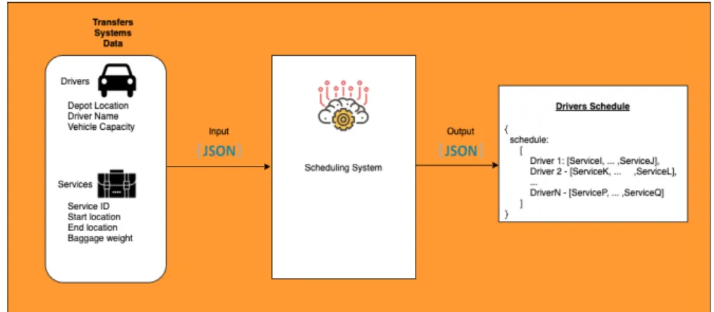
The figure 3.1 presents the system architecture. The transfer systems applications using pre booked methods have all the data about services and drivers stored. This input is required to the book a shuttle on the system implemented. The output provided is a list which assigns drivers to pre booked services. In terms of infrastructure, this can be integrated in any transfer app as a micro-service, which receives json and output json in a rest api. This can be used to notify drivers and the transfer system manager with the updated schedule.

3.2 Scheduling System Implementation

Figure 3.1: Automatic Scheduling System Architecture Diagram

3.2

Scheduling System Implementation

This problem can be seen as a constraint satisfaction optimization problem. To implement a solution for the automatic scheduling system the Google Or Tools library for Python was chosen.

This library offers Constraint Programming, which is a relatively new field. It has a CP-SAT solver which provides users functions to set variables, constraints and some predicates to optimize the results found.

An external API to get the traffic times between the geo-locations (drivers start point, services locations) was used to generate a matrix of traffic times as input in the scheduling algorithm, this way the time spent on generating the time matrix is separated from the time spent only in the scheduling function, even both make part of the scheduling system.

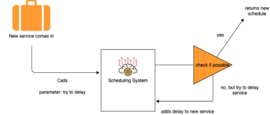
The way this system is implemented allows the re-scheduling function, as we can see in the figure 3.2.

The scheduling system has a configuration field which allows delays on the services. In case the schedule can’t be made for a certain input, the system retries a new schedule, increasing the starting time of the services by x minutes, and that gives a bit more flexibility to the drivers to get in time to the services.

3.2 Scheduling System Implementation

Figure 3.2: Scheduling System called recursively until it finds a solution

3.2.1

System Input

The system plans a schedule for drivers and services, obviously the system input needs parameters which give us information about both. These are the parameters needed for drivers:

• Depot location, this is the geo-location where the driver starts and finishes the daily journey. We need this because the system has to optimize the total time/distance driven, i.e, the driver will likely pick up a service that it’s closer from it start point as his first service, for instance.

• Driver name, this is required for the output so we can distinguish drivers. • Vehicle capacity, we have capacity constraints, so we need to know if the

driver vehicle has space enough to pick up a service.

The system also requires time and capacity constraints for services:

• Start time, the drive needs to be in the start location at the start time for each service.

• Start and end locations, the system needs the geo-location to calculate the distance/time for these services and to optimize the routes travelled by drivers.

3.2 Scheduling System Implementation

• Weight, each service has baggage allowed. There are lots of baggage allowed such as: travel bags, golf bags, bicycle, etc. One of the requirements is to make sure a driver can take passengers baggage and it is described on this field.

3.2.2

Variables

This optimization problem is using integers only to increase computational speed. Each driver will be a int variable. The system requires a list with services and a list with drivers. For each service, we need to create a dedicated variable that our program will assign as an integer, which represents the driver. Each service variable will be in the domain D_{∈ [1, ..., x], where x is the number of drivers.} # create variables for services

for service in services:

createIntVar(1, len(drivers))

A variable which saves the distance for each two services in a row is also created. It saves the distance from the service A to service B, if there isn’t a C between these two. As we can see in the pseudo-code below the distance to service A to B is set to null initially, and is set to its final value later. It doesn’t make sense to calculate distances for services that are not done in a row.

3.2 Scheduling System Implementation

3.2.3

Constraints

On a Capacitated Multiple Depot Vehicle Routing Problem With Time Window Constraints logically constraints for capacity, multiple depots and time windows need to be added to the model. Each driver has to depart from a starting point (which is usually home or a transfer shuttle depot), adding this constraint to the model, by assigning two new services to each driver : the starting service and the end service. Fundamentally we create two variables that oblige the first service for each driver to start at home and the service is made by himself.

Regarding capacity, it’s quite easy. We need to check the drivers vehicle capacity and service weight, if the vehicle capacity is greater or equal than the services then the driver can do this service.

3.2 Scheduling System Implementation

# Add weight constraints for s1 in services:

for driver in all_drivers:

if(driver.vehicle_capacity < s1.weight): addConstraint(s1 != driver)

Regarding the time window constraints, this must be satisfied by making sure the total time of a service is less then the start time of the next service, i.e, if the driver x is assigned to the services A and B, the total time (which includes doing the service A and also commute from the ending point at A to the starting point of B) is less than the starting time for the service B.

# Constraint to check if the driver can do the next service for s1 in services:

for s2 in services:

if (not(s1.total_time < s2.start_time)): addConstraint(s1 != s2)

3.2.4

Optimization function

The goal for the scheduling system, is to minimize the time a vehicle is in service without any passengers, i.e, it should minimize the sum of the times, where all the drivers have been moving from the previous service to the next, it’s called the wasted driven time and the goal is minimize this value. Implementing it using the Google or-tools, is quite tricky because we need the support of boolean variables. The algorithm checks if there are 3 service 1, 2 and 3 respectively, all assign to the same driver, so it verifies for each service it, the service 3 can happen between s1 and s2, i.e, the driver has time to finish the previous service and get to the next service, in time. If the service 3 can happen between 1 and 2, then the

3.2 Scheduling System Implementation

variable b is true and the distance is added to the distances array. After checking all the possible cases, the distances are minimized to ensure the drivers have the minimum wasted driven kilometers as possible.

b = model.NewBoolVar("") total_distance = [] for s1 in services: for s2 in services: if (not(s1.total_time < s2.start_time)): addConstraint(s1 != s2) for s3 in services:

if(s3.total_time < s1.start_time or s2.total_time < s3): pass else: addConstraint(s1 != s3).OnlyEnforceIf(b) addConstraint(s1 == s2).OnlyEnforceIf(b) if b: time_total = distance(s1,s2) else: time_total = 0 total_distance.append(time_total) Minimize(sum(total_distance))

Chapter 4

Experimental Results

To make the prove of concept of this system, two different sources of data are used: test data and real data. The test data was created initially and increased the complexity of the problem and consequently the system, as well. Thus, it started with a real small problem where the problem had three drivers, five services and the task assignment was quite simple. Regarding the real data, it was provided by a private transfers company where the services and drivers are real. In this chapter it is explained more, in depth, each scheduling problem and also the results for these experience.

4.1

Example test cases

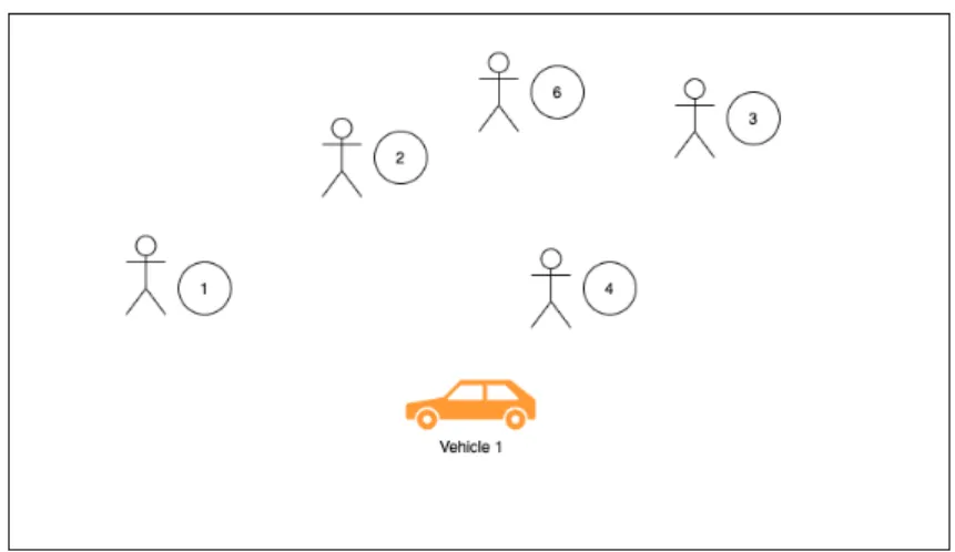
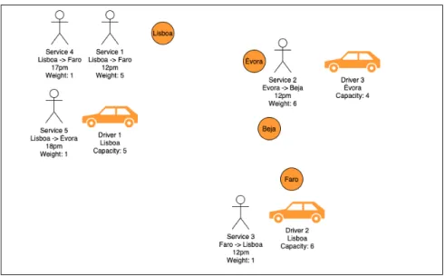
It’s quite simple to make a manual scheduling like the one presented in the figure 4.1, where we have three drivers and five services.

4.1 Example test cases

Figure 4.1: Test case problem image

To make sure the starting time and weight constraints are respected, this example manages to start three services at the same time, and it could be verified that the driver which is closer from a service is being assigned to that service, but only if it respects the weight constraints, i.e, if the driver have capacity to pick up a service with certain weight. The table 4.1, has the information about services:

Service Start Time Start Point End Point Weight Service 1 12h00m Lisboa Faro 5 Service 2 12h00m Évora Beja 6 Service 3 12h00m Faro Lisboa 1 Service 4 17h00m Lisboa Faro 1 Service 5 18h00m Lisboa Évora 1

Table 4.1: Test case Services

4.1 Example test cases

Driver Start Point Vehicle Capacity Driver 1 Lisboa 5

Driver 2 Faro 6 Driver 3 Évora 4 Table 4.2: Test case Drivers

The output makes total sense in this case because the aim is to minimize the times. Initially it makes sense the Driver 3 to be assigned to the Service 2, this is, the Driver who is from Évora be assigned to the service that starts in Évora, but because it doesn’t have capacity to support the service weight, the Driver 2 comes from Faro to do this service, the execution time for this test was 0.048 seconds and the minimized time is 484, considering the actual traffic time.

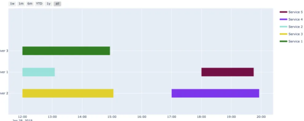
Figure 4.2: Automatic Scheduling for Example Test Case

The main goal in this system is to minimize the time when the drivers move from one service to the next, i.e, minimizing the time a driver drives without any passenger, when it is moving from home to the first service or moving from one service to another. To prove the system works as expected regarding time minimizing, was made a small change in the same problem presented in the figure 4.1, but setting the Driver 3 vehicle capacity to 6 so the service 2 can be done by this Driver and minimizing the time. The figure 4.3 presents the output making

4.1 Example test cases

this small change, resulting on the test case 2:

Figure 4.3: Automatic Scheduling for Example Test Case 2

It’s also important to see what happens in the case where there is no opti-mization. Test case 3 scheduling is presented in the Figure 4.4. Note the Driver 1 is picking up the Service 2, which is increasing the wasted time:

Figure 4.4: Automatic Scheduling for Example Test Case 3, without any opti-mization

Looking to the results on the table 4.3, the execution time is slightly lower on the test case 3, this is because the optimization function needs some time to process all the cases and to optimize the wasted driven time.

4.2 Real data test

Test Execution Time Wasted Driven Time

Test case 1 0.048 484

Test case 2 0.052 135

Test case 3 (no optimization) 0.038 335 Table 4.3: Test case results

4.2

Real data test

The services and drivers data was provided by a private and anonymous transfer company based in Algarve (Portugal), where the scheduling problem is done manually everyday. The aim is to confirm the implemented scheduling system perform so well as a person who is scheduling drivers manually. The table 4.4 contains the information about all the fifteen services provided by this company.

Service Start Time Start Point End Point Weight Service 1 17h30m Faro Albufeira 1 Service 2 09h00m Faro Praia da Rocha 6 Service 3 23h00m Faro Vilamoura 1

Service 4 19h00m Faro Lagos 1

Service 5 17h00m Albufeira Faro 5 Service 6 14h00m Albufeira Faro 1 Service 7 10h00m Faro Vilamoura 2 Service 8 14h30m Albufeira Faro 3 Service 9 08h00m Salgados Faro 1 Service 10 10h30m Faro Vilamoura 1 Service 11 11h00m Olhos de Água Faro 1 Service 12 16h30m Faro Porches 1 Service 13 13h30m Faro Carvoeiro 1 Service 14 13h30m Faro Quinta do Lago 2

Service 15 09h00m Lagoa Faro 1

4.2 Real data test

The table 4.5 contains the data about the five drivers: Driver Start Point Vehicle Capacity

Driver 1 Olhão 4

Driver 2 Faro 1

Driver 3 Albufeira 3

Driver 4 Faro 1

Driver 5 Albufeira (Guia) 5 Table 4.5: Real data test case drivers

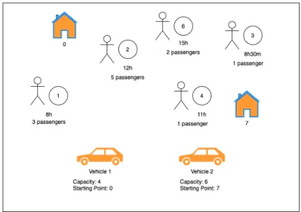
Looking to the figure 4.5 which is the daily schedule for all the drivers and services, the presented schedule is a feasible solution for this problem. Looking to the weight constraints, only the Driver 5 has vehicle capacity to do the Service 3. Looking for the starting points service, the algorithm always set the second service for the Drivers 2 or 4, because it’s the longest first journey and it assigns the Service to the Drivers based in Faro. To study the behaviour and performance of the algorithm used to solve this problem, the table 4.6 shows to different results for the same testing data. The goal here is to see, how long the optimization takes. It can be seen that the execution time of the program without optimization is very low, this is because the algorithm has a some constraints and to optimize the wasted driven time, the model has to make many calculations which exponencial increase with the number of drivers and services.

Test Execution Time Wasted Driven Time

Real data case 19.2 153

Real data case (no optimization) 2.657 428 Table 4.6: Real data test results

4.2 Real data test

Chapter 5

Conclusions

The capacitated and multiple depot vehicle routing problem with time constraints is a very actual problem in many sectors such as passenger transports, deliveries, street cleaning, door to door advertising, etc. On this dissertation it is proved that, systems can make use of Artificial Intelligence to solve this branch of the original vehicle routing problem, even using multiple and tricky constraints that exponentially increase the complexity of the problem. The presented schedule in the figure 4.5, which is a real data test is completely fine to be used as the schedule for the shuttle company on the mentioned day, and the objective was reached implementing the system using the Google OR-Tools technology. It was proved that Google OR-Tools enables to set constraints inside certain domains and also perform optimization to tackle constraint satisfaction problems.

5.1

Future work

The system was a proof of concept to tackle the vehicle routing problem, adding capacities on drivers vehicles and weights on services constraints. The drivers also have an initial depot, the starting point and the goal is to minimize the drivers time when they are not doing a service, i.e, when they are moving from one service to another. This is already a complex AI problem, but as future

5.1 Future work

work this complexity and difficulty can be increased. As future work, it can be added a finish route point to the Driver, so he can return to the company depot or home. Another feature that would improve the system is to add constraints so the vehicles are part of a company, I explain, if the company have different vehicles and the drivers can come back to the depot to change vehicle if needed. Another the feature that would bring more complexity and would make the system even more interesting for shuttle companies is to add is to give preference to a driver to pick up a defined service, because in some cases the drivers are paid by service, and of course the longest services mean more money for drivers. Balancing the schedule, i.e, remove drivers if they are not needed will be something to be added on the future work.

References

[1] J. Renaud, G. Laporte, and F. F. Boctor, “A tabu search heuristic for the multi-depot vehicle routing problem,” Computers & Operations Research, vol. 23, no. 3, pp. 229–235, 1996. 4

[2] S. Salhi and M. Sari, “A level composite heuristic for the multi-depot vehicle fleet mix problem,” European Journal of Operational Research, vol. 103, no. 1, pp. 95–112, 1997. 4

[3] K. C. Tan, L. H. Lee, Q. Zhu, and K. Ou, “Heuristic methods for vehicle routing problem with time windows,” Artificial intelligence in Engineering, vol. 15, no. 3, pp. 281–295, 2001. 4

[4] D. Karaboga, “An idea based on honey bee swarm for numerical optimiza-tion,” Tech. Rep. tr06, Erciyes university, engineering faculty, computer en-gineering department, 2005. 4

[5] D. Karaboga and B. Basturk, “Artificial bee colony (abc) optimization algo-rithm for solving constrained optimization problems,” in International fuzzy systems association world congress, pp. 789–798, Springer, 2007. 5

[6] B. Crevier, J.-F. Cordeau, and G. Laporte, “The multi-depot vehicle routing problem with inter-depot routes,” European journal of operational research, vol. 176, no. 2, pp. 756–773, 2007. 5

REFERENCES

[7] Q. Zhu, L. Qian, Y. Li, and S. Zhu, “An improved particle swarm opti-mization algorithm for vehicle routing problem with time windows,” in 2006 IEEE International Conference on Evolutionary Computation, pp. 1386– 1390, IEEE, 2006. 5

[8] B. Kallehauge, “Formulations and exact algorithms for the vehicle routing problem with time windows,” Computers & Operations Research, vol. 35, no. 7, pp. 2307–2330, 2008. 5

[9] R. Dondo and J. Cerdá, “A cluster-based optimization approach for the multi-depot heterogeneous fleet vehicle routing problem with time windows,” European journal of operational research, vol. 176, no. 3, pp. 1478–1507, 2007. 5

[10] R. G. Dondo and J. Cerdá, “A hybrid local improvement algorithm for large-scale multi-depot vehicle routing problems with time windows,” Computers & Chemical Engineering, vol. 33, no. 2, pp. 513–530, 2009. 5

[11] Y. Xu, L. Wang, and Y. Yang, “A new variable neighborhood search algo-rithm for the multi depot heterogeneous vehicle routing problem with time windows,” Electronic Notes in Discrete Mathematics, vol. 39, pp. 289–296, 2012. 5

[12] M. Mirabi, N. Shokri, and A. Sadeghieh, “Modeling and solving the multi-depot vehicle routing problem with time window by considering the flexible end depot in each route,” International Journal of Supply and Operations Management, vol. 3, no. 3, p. 1373, 2016. 5

[13] G. B. Dantzig and J. H. Ramser, “The truck dispatching problem,” Manage-ment science, vol. 6, no. 1, pp. 80–91, 1959. 6

REFERENCES

[14] “Google or-tools: The bin packing problem.” https://developers.google. com/optimization/bin/bin_packing#python_5. Accessed: 2019-04-28. 10 [15] S. Sumathi, L. A. Kumar, et al., Computational Intelligence Paradigms for Optimization Problems Using MATLAB ¯U/SIMULINK ¯U. CRC Press, 2018. [16] S. R. Thangiah, “A hybrid genetic algorithms, simulated annealing and tabu

search heuristic for vehicle routing problems with time windows,” Practical handbook of genetic algorithms, vol. 3, pp. 347–381, 1999.

[17] J. Pearson and P. G. Jeavons, “A survey of tractable constraint satisfaction problems,” tech. rep., Technical Report CSD-TR-97-15, Royal Holloway, Uni-versity of London, 1997.

[18] Z. Liu, Algorithms for constraint satisfaction problems (CSPs). PhD thesis, University of Waterloo Canada, 1998.