Study of the relationship between rainfall, runoff and land
use in five watersheds
Drought and impacts on the landscape system
Luís Miguel Custódio Tangarrinha
Dissertation for obtaining Master degree in
Landscape Architecture
JURI:
PRESIDENTE - Doutora Maria Isabel Freire Ribeiro Ferreira, Professora Catedrática do Instituto Superior de Agronomia da Universidade de Lisboa.
VOGAIS - Doutor Francisco Manuel Cardoso de Castro Rego, Professor Associado com agregação do Instituto Superior de Agronomia da Universidade de Lisboa, orientador;
- Doutora Ana Luísa Brito dos Santos Sousa Soares Ló de Almeida, Professora Auxiliar do Instituto Superior de Agronomia da Universidade de Lisboa.
AGRADECIMENTOS
Em primeira instância, o maior agradecimento vai para o excepcional orientador que me deu a honra de com ele trabalhar, o Professor Francisco Castro Rego. Agradeço também pela dedicação, conhecimento inesgotável e capacidade de trabalho que entregou a este trabalho. Depois, agradecer também a dedicação e ajuda que a Susana Dias sempre entregou a este trabalho, que por isso também é seu.
À Marta Rocha, por me der cedido os dados de ocupação de solo e por sempre ter estado à disposição para aquilo que precisei ao longo do trabalho.
Ao Diogo Raposo, que me acompanhou na aventura brasileira, onde estudei Ecologia na Universidade Federal do Rio Grande do Norte, e onde aprendi conhecimentos bastante importantes para este trabalho.
À Margarida Coimbra pela a incansável disponibilidade no auxilio na escrita deste trabalho, em inglês.
Àqueles com quem tive oportunidade de trabalhar na direção da AEISA e que bastante força me deram ao longo deste tempo para que concluísse com sucesso este trabalho.
Àqueles com quem partilhei casa e que sempre tiverem mais paciência para mim nos momentos mais dificieis, o André Godinho, o Nuno Pinto e o Simão Afonso.
Ao Mister Alberto Gonçalves, por ter sido como um padrinho, e sempre me ter acompanhado e ajudado ao longo de todo o meu percuso académico.
Depois, importante também agradecer a todos os meus amigos que sempre estiveram a meu lado e sempre me apoiaram nos momentos mais difíceis.
Para acabar, dedico este trabalho aos meus pais, Ester e Martinho, ao meu irmão, João, aos meus avós, José, Ercilia, Agostinho e Inácia.
E por fim, dedicar este trabalho àquele que mais força me deu e a quem, por mais que o tempo passe nunca poderei esquecer. João Pedro Dinis, colega de casa, amigo e grande companheiro que nos deixou no ano passado mas que para sempre estará no meu coração.
ABSTRACT
The amount of water generated from a watershed depends on the climate, soils, geology, vegetation and land use. Water inputs of precipitation as rain are divided by watershed in the evapotranspiration, runoff and groundwater recharge. This study examined the factors that can affect the runoff of Portuguese watersheds, focusing on factors related to land and watershed management.
For this analysis, a methodology developed by Thornthwaite-Mather was used to compute streamflow with the input of precipitation and temperature obtained by Portuguese Meteorology Services. These data were compared with the observed values in order to be able to calculate soil properties, in this case, the values of coefficient of reservoir and available water content. These values are possibly related to changes in the composition of the soil and were compared with the values of land use for periods studied based on CORINE methodology (1970 to 2006).
The existence of periods of drought, calculated with SPI-12months and their impacts were also compared with changes in soil and land use.
These processes are the main steps for understanding the changes that affect all these systems. These changes are important for the planning future landscape management.
RESUMO
A quantidade de água gerada a partir de uma bacia hidrográfica depende do clima, solos, geologia, cobertura vegetal, e uso do solo. Os inputs de água provenientes da precipitação, como a chuva, são divididos pela bacia hidrográfica em evapotranspiração, escoamento superficial e recarga de aquíferos. Este estudo analisou os fatores que afetam o escoamento nas bacias hidrográficas, focando fatores relacionados com o solo e à gestão de regiões hidrográficas.
Na análise, é utilizada uma metodologia desenvolvida por Thornthwaite-Mather em que foram comparados dados de escoamento estimando a partir da precipitação e temperatura atribuído pelos Serviços Portugueses de Meteorologia. Os dados são comparados com os valores reais do Serviço Português de Meteorologia de escoamento de modo a calcular as propriedades do solo, como os valores de coeficiente de reservatório e do teor de água disponível. Estes valores estão relacionados com mudanças na composição do solo e são comparados com os valores de ocupação de solo para vários períodos de tempo com base na metodologia CORINE (de 1970 a 2006). A existência de períodos de seca, calculados com SPI-12 (Índice de Precipitação Padrão) e os impactos são também comparados com as alterações do solo e sua ocupação.
Palavras-Chave: Bacia hidrográfica, Seca, Ocupação de solo, Thornthwaite-Mather,
RESUMO ALARGADO
A paisagem encontra-se em constante mudança e a sua dinâmica pode ser entendida como um processo de transformação das relações estabelecidas entre os elementos que a compõem. Para a compreender, é assim necessário, identíficar os fatores que vêm a determinar a sua transformação. Assim sendo, a maneira como esta é naturalmente ou artificialmente transformada irá afetar toda a sua dinâmica num determinado período de tempo.
A quantidade de água gerada a partir de uma bacia hidrográfica depende do clima, dos solos, da geologia, da cobertura vegetal, e do uso do solo. Os inputs de água proveniente da precipitação na forma de chuva ou neve são divididos pela bacia hidrográfica em evapotranspiração, escoamento superficial e recarga de aquíferos.
Neste estudo concreto, são analisados os fatores que podem afetar o escoamento nas bacias hidrograficas portuguesas com foco em fatores relacionados com a climatologia, os solos, e a gestão dada ao uso do solo existente nestas bacias. Torna-se então imprescindível compreender estas mudanças (que podem ser as mais variadas, desde do reflorestamento, ao desmatamento, à criação de solos agrícolas, ao uso urbano e ao impacto do escoamento superficial).
Para poder compreender as mudanças de uso no solo foi utilizada a metodologia do balanço de água no solo, desenvolvido por Thornthwaite-Mather, nos quais foram utilizados os dados de precipitação e temperatura retirados dos Serviços Portugueses de Meteorolgia (Instituto Português do Mar e da Água). Após a entrada destes dados no modelo, são calculados os valores de escoamento através deste modelo de Thornthwaite-Mather, e comparados com os valores reais provenientes, também, dos Serviços Portugueses de Meteorologia. Após esta comparação, serão otimizados os valores referentes às propriedades do solo (teor de água disponível e o coeficiente de escoamento). Estes valores são comparados com os valores de ocupação do solo para os vários periodos de tempo com base na metodologia CORINE (neste caso para os anos 1970, 1990, 2000 e 2006).
Depois são calculados os períodos de seca, através do cálculo dos valores de SPI (Índice de Precipitação Padrão) e discutidos os seus possíveis impactos na ocupação de solo.
ÍNDICE
ABSTRACT ... II RESUMO ... III RESUMO ALARGADO ... IV LIST OF FIGURES AND TABLES ... VII LIST OF ABBREVIATIONS ... X DISSERTATION FRAMEWORK ... 1 1. INTRODUCTION ... 3 1.1. Hydrologic Cycle ... 5 1.2. Drainage basin ... 6 1.2.1. Geometric characteristics ... 8 1.2.2. Relief characteristics ... 9
1.3. Portuguese water legislation ... 9
1.3.1. Management Plan of Hydrographical Region ... 10
1.4. General definitions ... 11
1.4.1. Precipitation ... 11
1.4.2. Evapotranspiration (ET) ... 14
1.4.3. Potential evapotranspiration (ETP) ... 15
1.5. Thornthwaite-Mather method ... 15
1.5.1. Actual Evapotranspiration (AET) ... 17
1.5.2. Surplus ... 18
1.5.3. Accumulated Potential Water Loss (APWL) ... 18
1.5.4. Deficit ... 18
1.5.5. P minus PE (P-PE) ... 18
1.5.6. Soil water and change in soil water (SW and ΔSW) ... 18
1.5.8. Detention ... 19
1.5.9. Actual flow ... 19
1.5.10. Available water capacity (AWC) ... 19
1.5.11. Coefficient of reservoir (f) ... 19 1.6. Drought ... 19 1.7. Cultural coefficient (Kc) ... 24 2. METHODS ... 26 2.1. Study area ... 26 2.1.1. Dataset ... 26 2.1.2. Geographic location ... 30 2.2. Thornthwaite-mather method ... 31
2.3. Trends in annual precipitation and streamflow... 31
2.4. Analysis of coefficient of reservoir (f) and available water capacity (AWC) ... 31
2.5. Land use ... 32
2.6. Drought analysis ... 34
2.7. SCS curve number ... 35
3. RESULTS ... 39
3.1. Annual Precipitation and Streamflow ... 39
3.2. Comparison between precipitation and runoff (real and simulated) ... 42
3.3. Analysis of soil proprieties ... 49
3.4. Land use ... 56
3.5. Relationship between AWC, f and land used ... 59
3.6. Drought analysis ... 60
3.7. SCS curve number ... 61
4. CONCLUSIONS ... 62
LIST OF FIGURES AND TABLES
Figures
Figure 1 - Hydrologic System scheme (Jackson, 2008) ... 5
Figure 2 - Scheme of Hydrological System ... 7
Figure 3 - Hydrographic regions of Portugal (Azinhal Algarve, 2008) ... 10
Figure 4 - Thiessen method (scheme) ... 12
Figure 5 - Determination of B polygon ... 12
Figure 6 - Determination of point where the level curves will pass ... 13
Figure 7 - The partitioning of evapotranspiration into evaporation and transpiration over the growing period for an annual field crop ... 14
Figure 8 - The soil reservoir and how it connects to stream discharge at the watershed outlet, Q0 (Chen , Gao, Guo, & Ren, 2005) ... 16
Figure 9- Drought (Inthecapital, 2012) ... 20
Figure 10 - Drought definitions (National Drought Mitigation Center) ... 22
Figure 11 - Location of selected catchments and meteorological stations (Rego, Acácio, Van Lanen, & Stahl, 2013) ... 30
Tables Table 1 - Morphometric characteristics and type of analyses for drainage basin ... 7
Table 2 - Situation (of dry/wet) in watershed (Chen , Gao, Guo, & Ren, 2005) ... 17
Table 3 - Classification of water shortages ... 21
Table 4 - Characterization of selected meteorological stations and precipitation dataset . 28 Table 5 - Characterization of selected gauging stations and streamflow dataset ... 29
Table 6 - Portuguese Meteorological Service (Institute of Meteorology) dataset information of watersheds ... 29
Table 7 - (CORINE Land Cover (CLC) nomenclature ) ... 32
Table 8 - Runoff curve numbers for urban areas (USDA-SCS, 1985) ... 36
Table 9 - Runoff curve numbers for cultivated agricultural lands (USDA-SCS, 1985) ... 37
Table 10 - Runoff curve numbers for other agricultural lands (USDA-SCS, 1985) ... 38
Table 11 - Runoff curve numbers for arid and semiarid rangelands (USDA-SCS, 1985) . 38 Table 12 - Variation of soil properties with latitude ... 39
Table 13 - Ranges of average annual precipitation and actual flow in the whole data period in Gimonde, Bragança ... 40
Table 14 - Ranges of average annual precipitation and actual flow in the whole data
period in Vale Giestoso, Porto ... 40
Table 15 - Ranges of average annual precipitation and actual flow in the whole data period in Manteigas, Coimbra. ... 41
Table 16 - Ranges of average annual precipitation and actual flow in the whole data period in Pavia, Lisboa. ... 41
Table 17 - Ranges of average annual precipitation and actual flow in the whole data period in Vascão, Beja... 42
Table 18 – Gimonde, Comparison between precipitation and runoff (real and computer) 1966-1980 ... 43
Table 19 – Gimonde, Comparison between precipitation and runoff (real and computer) 1980-2000 ... 43
Table 20 - Gimonde, Comparison between precipitation and runoff (real and computed) 2000-2004 ... 44
Table 21 - Vale Giestoso, Comparison between precipitation and runoff (real and computed) 1957-1980 ... 44
Table 22 - Vale Giestoso, Comparison between precipitation and runoff (real and computed) 1980-1990 ... 45
Table 23 - Manteigas, Comparison between precipitation and runoff (real and computed) 1948-1980 ... 45
Table 24 - Manteigas, Comparison between precipitation and runoff (real and computed) 1980-1996 ... 46
Table 25 - Pavia, Comparison between precipitation and runoff (real and computed) 1952-1980 ... 46
Table 26 - Pavia, Comparison between precipitation and runoff (real and computed) 1980-1990 ... 47
Table 27 - Vascão, Comparison between precipitation and runoff (real and computed) 1960-1980 ... 47
Table 28 - Vascão, Comparison between precipitation and runoff (real and computed) 1980-2000 ... 48
Table 29 - Vascão, Comparison between precipitation and runoff (real and computed) 2000-2011 ... 48
Table 30 - Correlation values for Gimonde for the whole period (1966-2004) ... 49
Table 31 - Correlation values for Gimonde for the interval between 1966 and 1980 ... 49
Table 32 - Correlation values for Gimonde for the interval between 1980 and 2000 ... 49
Table 34 - Best values of AWC and f obtained from correlations of Gimonde basin ... 50
Table 35 - Correlation values for Vale Giestoso for the whole period (1957-1990) ... 50
Table 36 - Correlation values for Vale Giestoso for the interval between 1957 and 1980 ... 51
Table 37 - Correlation values for Vale Giestoso for the interval between 1980 and 1990 ... 51
Table 38 - Best values of AWC and f obtained from correlations of Vale Giestoso basin . 51 Table 39 - Correlation values of Manteigas for the whole period ... 51
Table 40 - Correlation values for Manteigas for the interval between 1948 and 1980 ... 52
Table 41 - Correlation values for Manteigas for the interval between 1980 and 1996 ... 52
Table 42 - Best values of AWC and f obtained from correlations in the Manteigas basin . 52 Table 43 - Correlation values of Pavia for whole period (1952-1980)... 52
Table 44 - Correlation values for Pavia for the interval between 1952 and 1980 ... 53
Table 45 - Correlation values for Pavia for the interval between 1980 and 1990 ... 53
Table 46 - Best values of AWC and f obtained from correlations in the Pavia basin ... 53
Table 47- Correlation values of Vascão for the whole period (1960-2011) ... 53
Table 48 - Correlation values for Vascão for the interval between 1960 and 1980 ... 54
Table 49 - Correlation values for Vascão for the interval between 1980 and 2000 ... 54
Table 50 - Correlation values for Vascão for the interval between 2000 and 2006 ... 54
Table 51 - Best values of AWC and f for correlations of Vascão basin ... 54
Table 52 - Relation between f value and actual flow ... 55
Table 53 - Relation between AWC and actual flow ... 55
Table 54 - Percentage of land used by each class in the Gimonde basin ... 56
Table 55 - Percentage of land used by each class in the Vale Giestoso basin ... 56
Table 56 - Percentage of land used by each class in the Manteigas basin ... 57
Table 57 - Percentage of land used by each class in the Pavia basin ... 57
Table 58 - Percentage of land used by each class in the Vascão basin ... 58
Table 59 - Balance of land used ranges in all studied periods ... 58
Table 60 - Relationship between the best AWC and f values optimized and land used ... 59
Table 61 - Drought category and values used to calculate the drought magnitude ... 60
LIST OF ABBREVIATIONS
AET – Actual evapotranspiration
APA – Portuguese Environment Agency APWC – Accumulated potential water loss AWC – Available water capacity
CORINE – Coordination of information on the environment DL – Drought month duration
DM – Drought magnitude
DMM – Drought average magnitude ET – Evapotranspiration
ET0 – Reference evapotranspiration
ETP – Potential evapotranspiration
f – Coefficient of reservoir
FAO – Food and Agriculture Organization of United Nations INAG – Portuguese Water Institute
Kc – Cultural Coefficient
RH – Hydrographic region
SNIRH – National Information System in Hydric Resources SPI – Standard precipitation index
SWB – Soil water balance
0. Dissertation framework
Starting with justification why this dissertation is written in English. This dissertation was incorporated in the DROUGHT R&SPI project.
Drought is natural hazard that has hit Europe hard over the last decades. Likely it will become more frequent and severe and the scale will increase due to the increased likelihood of warmer Northern winters and hotter Mediterranean summers. There is an urgent need to improve drought preparedness through increased knowledge on the past and future hazard, impacts, and possible management and policy options, measures, and through drought management plans and an improved science-policy interfacing. This will reduce vulnerability to future drought and the risks they pose for Europe. DROUGHT-R&SPI will address this pressing need. (Lanen, 2013).
The main project objectives are:
Drought as a natural hazard, including climate drivers, drought processes and occurrences;
Environmental and socio-economics impacts;
Vulnerabilities, risks and responses.
Lisbon, October de 2013
Drought R&SPI Project
1. INTRODUCTION
The hydrologic system is complex and it extends through all the parts of the earth’s system. The landscape system is a part of the earth’s system and it’s dynamic components need to be the key for its own planning. One of the main targets of this study is to understand in which way the hydrographic system is related with the landscape system. In watersheds, there are components of the landscape that are modeled by the hydrological system as vegetation and soil.
The following thematic study: Landscape planning and vulnerability assessment in the Mediterranean brings attention to the methodologies used in spatial planning, in particular landscape planning approaches that allow the integration of various land uses and protection of landscape values through planning instruments.
To efficiently fulfill the new tasks, the landscape planning functions should be optimally coordinated with other relevant planning and assessment instruments. Due to pending and anticipated changes, the continuation and updating of landscape planning will be particularly important. Flexible, modular and conclusive digital processing, which is aimed at problem related planning statements oriented to the need for action, is indispensable for this.
The main purpose of this project is to find linkages between landscape system, land use, and precipitation-runoff relationships, that let us know the consequences of landscape changes in hydric behavior of watersheds.
“A few studies have so far been published on the effect of climate change on the impacts of drought in water resources terms at the local catchment scale, and there are no reported studies on the relation between precipitation and stream flow trends specifically for Portugal, which is considered one of the areas of the Iberian Peninsula most affected by significant climatic changes”. (Rego, Acácio, Van Lanen, & Stahl, 2013).
Starting from this principle, there was some concern about starting to study more this issue. In order to understand this problem, few water balance models were studied. In this specific case the model used was a very simple mode, the Thornthwaite-Mather water balance model because it is possible to calculate the runoff using precipitation, temperature and with it latitude. Since one of the main targets of this study is planning the landscape and a comparison between the calculated values obtained through the Thorthwaite-Mather soil water balance model with the actual flow data from the Portuguese Meteorological Service (Institute of Meteorology) was done. After comparing
all these values, it is necessary to optimize the variables soil characteristics as well as the available water capacity and coefficient of reservoir. These values will be optimized during the study, making it possible to find a range on the soil’s response to water. Being this response an important step to understand some ranges in land use.
Using land use data from Forestry National Inventory of some strategic periods as 1970, 1990, 2000 and 2006 and using the CORINE legend(Coordination of information on the environment) it was created a new scale for better understanding of the relationship of the most abundant classes of used data. To study the dynamic of landscape system it is necessary to compare the effect of water on soil’s response, ranging the land use.
It also important to study the drought impacts and modifications on the landscape system. Using the Standard Precipitation Index to calculate the magnitude of the drought, to split the classes where the water shortage is more aggressive. After that it is also important to compare the main droughts calculated with land use range.
By the way, landscape ecology is a science that tries to explain the operation of landscape system and the landscape architecture as the main target of make an intervention in landscape system for improve his operations.
1.1. Hydrologic Cycle
The hydrological cycle (figure 1) is usually called a recurring consequence of different forms of movement of water and changes of its physical state in the nature on a given area of the earth (a river or lake basin, a continent or the entire earth). The movement of water in the hydrological cycle extends through the four parts of the Earth’s total system – atmosphere, hydrosphere, lithosphere, and biosphere – and strongly depends on the local peculiarities of these systems. The terrestrial hydrological cycle is of a special interest when referring to mechanism of formation of water resources on a given area of the land. Taking into account its global climate and other geophysical processes, the global hydrological cycle is often considerated. It is obvious that the role of different processes in the hydrological cycle in their description have to depend on the closer spatial-temporal scales. (Kuchment, 2001).
The total amount of water on Earth is divided in three phases that have kept constant since the appearance of man: solid, liquid and gaseous. It is also divided into three main reservoirs: oceans, continents and the atmosphere, among which there is a continuous circulation in a process called Hydrological Cycle. (Pinto, Holtz, & Martins, 1973). In liquid and solid forms, the water covers more than two thirds of the land’s surface, but in its gaseous form it is considerate a variable component of the atmosphere (which can take up to 4% of the whole volume). Under such conditions, water vapor is in its major quantity in the tropics and in the lower layers of the atmosphere. (Camargo, 2005). Water is composed by molecules that attract one another by the force of cohesion. These molecules in the liquid state are in constant motion, moving vertically towards the atmosphere and horizontally towards the surface. This movement is proportional to the energy or temperature of water. If the temperature increases, the rougher surface molecules tend to escape of the liquid water mass and keep the atmosphere free in its gaseous state. If the temperature of liquid water decreases, the movement of the molecules decreases as well. If the temperature reaches zero centigrade, the water molecules are fixed and solidify, forming ice. So, the Hydrological Cycle is composed by a
Figure 1 - Hydrologic System scheme (Jackson, 2008)
succession of various processes in nature, where the water starts going in a typical way on an early stage, to return to its original position. This global phenomenon of closed circulation of water between the land surface and the atmosphere is fundamentally driven by radiant energy and associated with terrestrial gravity and rotation. It is estimated that about 10% of the total vapor is used to recycle.
The land surface that covers the continents and oceans , such as the porous layer overlying continents (soils, rocks) and the reservoir formed by lakes, the rivers and the oceans take part in the whole hydrological cycle. Part of it is formed by the circulation of water on the surface itself and by the movement of water in and on the surface of the soil, rocks, lakes and other liquid surfaces and living things (such as animals and plants).
1.2. Drainage basin
Playfair (1802) described drainage basins as trees, where each stream would delicately be adjusted such that at each joining of streams, the slopes would delicately be balanced. The systematic change of the slope within landscapes suggested to Playfair that the equilibrium between erosion and sediment transport over the entire basin, and a stable geometry would result from this balance. Another author, Gilbert (1977), noted that erosional landforms have convergent stream networks and divergent ridge networks, and proposed that the typical concave-up profile of streams is due to the increased volume of water moving through downstream sections into the drainage network. He postulated that gaps between adjacent streams must migrate toward the stream with a shallower gradient; stable channel networks are achieved once gradients in adjacent streams are similar. The instability of drainage lines could be explained in terms of differential resistance to erosion, differential uplift, time and, possibly, the interaction between stream transport capacity and availability of sediment for transport. For Gilbert, the network of streams and hill slopes is a strongly interactive system, carefully adjusted to the dynamic equilibrium into a stable form (Gilbert, 1877). Strahler (1950) characterized erosional landscapes as open mass-transport systems that adjust their morphology to attain a time-independent form. He measured valley-side slope angles from several completely dissected natural drainages, and showed that a given area maintains a characteristic slope with a narrow range of values. The presence of a characteristic slope lends support to the hypothesis of a stable landform (Strahler, 1950). Hack hypothesized that every stream hill slope pair is adjusted one to the other, and, given constant forcing conditions, all elements of the landscape erode at the same rate, similar to Gilbert’s dynamic
equilibrium. Differences in form could, under those conditions, be related only to differences in resistance to flow, such as variable lithology and vegetation. Changes in the form could also result from different forcing conditions, even thou responses to perturbations are fast enough to restore a dynamic steady state adjusted to the new boundary conditions. He explicitly
viewed landscapes as spatial structures with time-independent forms. (Hack, 1960).
Figure 2 shows a scheme of hydrological system.
For Tonello (2005), the morphometric characteristics can be divided in: geometrics, land relief and drainage, shown on table 1.
Morphometric characteristics Type of analyses
Geometric characteristics
Total shape area Total perimeter
Coefficient of Compactness (Kc) Form factor (F)
Circularity index (IC) Drainage pattern
Land relief characteristics
Orientation Minimum slope Medium slope Maximum slope Minimum altitude Medium altitude Maximum altitude
Medium slope of main watercourse
Drainage characteristics
Length of main watercourse Total length of watercourse Drainage density
Order of watercourses Table 1 - Morphometric characteristics and type of analyses for drainage basin
1.2.1. Geometric characteristics
a) Area: Total area drained by the river system included among its topographic dividers, designed in the horizontal plane, being a basic element for the calculation of various morphometric indices.
b) Perimeter: Length along the imaginary line of splitter waters.
C) Form Factor (F): It compares the shape of the basin with a rectangle, corresponding to medium width ratio between the medium width and the axial length of the basin (from the river mouth to the furthest point of the river spike) and may be influenced by some features, mainly by geologic factors. It can also change due to some of hydrological processes on the hydrologic behaviour of basin. The form factor can be described by the following equation:
𝐹 =
𝐴
𝐿
2Where, F = Form factor; A = Drainage area; L = Axis length of the basin
d) Coefficient of compactness (Kc): Lists the shape of the basin with a circle. Is the ratio between the perimeter of the basin and the circumference of a circle of equal area as the basin. This coefficient is a dimensionless number which varies with the shape of the basin, regardless its size. The more irregular the basin is, the higher the coefficient of compactness. A minimum coefficient equal to one unit corresponds to a circular basin and for an elongated basin, its value is significantly greater than one, and may be calculated by the following equation:
𝐾𝑐 = 0,28 ×
𝑃
√𝐴
Where, Kc = Coefficient of compactness; P = Perimeter; A = Drainage area
e) Circularity index (IC): Simultaneously with the coefficient of compactness, the circularity index tends to the unity as the basin approaches the circular shape, and decreases as the shape becomes elongated, according to the equation:
𝐼𝐶 =
12,57 × 𝐴
𝑃
2f) Drainage pattern: Is the relationship between the number of rivers or watercourses and the catchment area expressed as follows:
𝐷ℎ =
𝑁
𝐴
Where, Dh = Drainage pattern; N = Number of rivers or watercourses; A = Drainage area The target of this index is to compare the frequency or the amount of existing watercourses area in a standard size, such as square kilometer.
1.2.2. Relief characteristics
a) Slope: The slope is related to the speed that gives superficial runoff therefore affecting the time it takes for the water from the rain to concentrate on riverbeds. This constitutes the drainage network basins, with the peaks of flood, infiltration and susceptibility to soil erosion depending on the speed with which the flow occurs on the land basin.
b) Altitude: The altitude variation is associated to precipitation, evaporation and transpiration and thus on average runoff. Great variations of a basin altitude cause significant differences in medium temperature, and it causes variations in the evaporation. More significant, however, are the possible variations of annual precipitation with elevation.
c) Amplitude altimetry: is the variation between the maximum altitude and minimum altitude.
1.3. Portuguese water legislation
The Portuguese water law (Portuguese Law n.º 58/2005, of 29th December), which transposes into national law the EU Water-Framework Directive (Directive no. 2000/60/EC of 23th October), establishes the framework for the management of surface water, including inland waters, transitional, coastal and underground waters.
The main unit for management of watersheds is the river basin district (was the basin), which corresponds to the area of land and sea, made up of one or more contiguous watersheds and underground water’s and coastal and their associated.
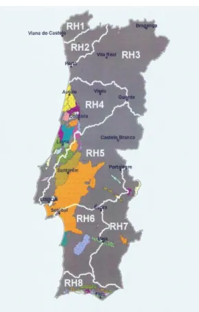
The Portuguese water law establishes 8 river hydrographic regions (RH) in Portugal, whose boundary is defined by normative geo referenced own, present on figure 3.
The river basin is also the main planning unit of water, being this achievement possible due to the use of three instruments, in particular through the Management Plans Hydrographical Region (PGRH).
1.3.1. Management Plan of Hydrographical Region
The Management Plan of Hydrographical Region, whose content is defined in art. 29 of the Portuguese water law, pretends to establish the basis of support for management, protection and appreciation of the environmental, social and economic waters. These plans cover watershed’s integrated river basin districts, estuaries, coastal areas and associated aquifers.
According to the decree-law that defines the content of Management Plan of Hydrographical Region, these will have to be mandatorily incorporated in the Master Plans in order to function as regulatory instruments of relations between the administration and citizens as well as agents of socio-economic development, in relation to the Water.
The Management Plan of Hydrographical Region will include a general description of the river basin, a characterization of natural pressures and impacts related to human activity, and a significant program of measures to ensure the continuation of the environmental objectives set out in the Portuguese Water Law. (Rosas).
Figure 3 - Hydrographic regions of Portugal (Azinhal Algarve, 2008)
1.4. General definitions
1.4.1. PrecipitationPrecipitation is the water that reaches the Earth's surface from the water vapor in the atmosphere, in the form of rain, sleet, snow and dew. The quantitative characteristics of rainfall measurements are: (Pedrazzi)
Height rainfall - rain measures made in the rain gauges and expressed in millimeters. Is the water depth to be formed on the soil as a result of some rain, if there were no runoff, infiltration or evaporation of the precipitated water;
Duration - the period of time starting from the beginning to the end of precipitation, usually expressed in hours or minutes;
Precipitation intensity - is the ratio between the height and duration of rain precipitation expressed as mm / h or mm / min.
Medium precipitation over a basin
To calculate the average precipitation of any surface, it is necessary to use the comments of the posts within that area and its neighborhoods.
There are three methods to calculate the average rainfall: • Method of Arithmetic mean;
• Method of Thiessen; and • Method of Isoietas. Method of Arithmetic mean:
Arithmetic mean consists on the sum of precipitation observed in positions that are inside of the basin being the result divided by their number.
This method is only recommended for basins smaller than 5000 km, with rain gauges evenly distributed on a flat area or gentle slope.
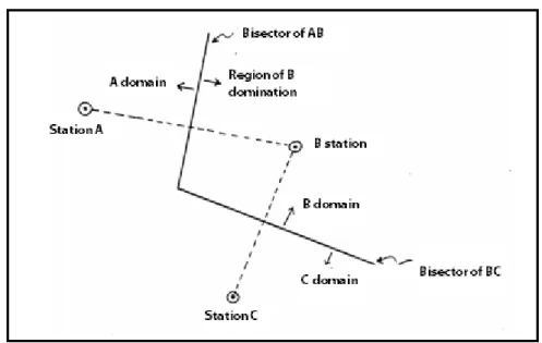
Method of Thiessen
Thiessen polygons are areas of "domain" of a rainfall station. It is considered that within these areas is the same precipitation altitude of the respective post. The polygons are drawn as follows:
Figure 4 - Thiessen method (scheme)
1st. Two adjacent stations are connected for a line (figure 4);
2nd. Traces the bisector of this line. This bisector divides from one side to another, the
regions of "domain".
3rd This procedure is initially performed by any position (for exemple, station B),
connecting it to the adjacent. It is defined in this way, the polygon of that position (figure 5).
Figure 5 - Determination of B polygon
4th. Repeat the same procedure for all stations.
5th. Disregard the areas of the polygons that are outside the basin.
𝑃̅ =
∑
𝐴𝑖𝑃𝑖
𝑛 𝑖=1
𝐴
𝑷
̅ , is the medium precipitation on the basin (mm)
𝑷𝒊 , is the precipitation on the station (mm)
𝑨𝒊 ,
it’s the shape area of the polygon inside the basin (km2)A, it’s the total area of the basin (km2). Method of Isoietas
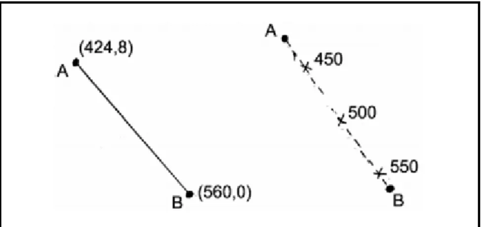
Isoietas method are indicative lines of the same height rainfall. Spacing lines can be set based on the type of study being developed and may be 5 by 5 mm, 10 by 10 mm, etc. Isoietas need to be drawn up in the same way as the counter lines in topography in the presence of rainfall in some raised stations.
The Isoietas method is established by following steps:
1st. define the desired spacing between the Isoietas;
2nd. connects with a semi-line, two adjacent stations, putting their respective rainfall
heights;
3rd. interpolates linearly determining the points where they will pass the level curves,
within the range of two heights rainfall (figure 6).
Figure 6 - Determination of point where the level curves will pass
4th. proceed that way with all the adjacent rain gauges;
6th. the medium rainfall is calculated by the following equation:
𝑃̅ =
∑
𝑃𝑖 . 𝐴1
̅̅̅̅̅̅̅̅̅̅̅
𝑛 𝑖=1
𝐴
𝑃̅ , medium precipitation on basin
𝑃̅𝑖 , arithmetic means of two followed isoietas “I” and i+1”
Ai , is the shape area of the basin between two respected isoietas (km2) A , is the total area of basin (km2)
1.4.2. Evapotranspiration (ET)
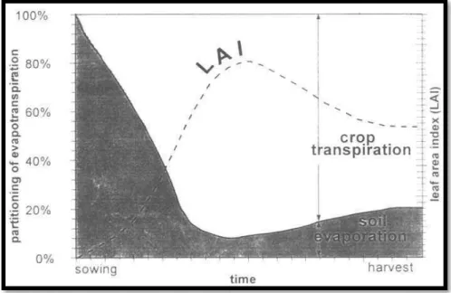
Evaporation and transpiration occur simultaneously and there is no easy way of distinguishing between the two processes. Apart from the water availability in the topsoil, the evaporation from a cropped soil is mainly determined by the fraction of the solar radiation reaching the soil’s surface. This fraction decreases over the growing period as the crop develops and the crop’s canopy shades cover more and more the ground’s area. When the crop is small, water is predominately lost by soil evaporation, but once the crop is well developed and completely covers the soil, transpiration becomes the main process. In Figure 7 the partitioning of evapotranspiration into evaporation and transpiration is plotted in correspondence to leaf area per unit surface of soil below it. At sowing nearly 100% of ET comes from evaporation, while at full crop cover more than 90% of ET comes from transpiration. (Allen, Pereira, Raes, & Smith, 1998)
Figure 7 - The partitioning of evapotranspiration into evaporation and transpiration over the growing period for an annual field crop
1.4.3. Potential evapotranspiration (ETP)
Potential evapotranspiration (ETP), according to Penman (1956), is the total amount of water for a large area completely covered with vegetation stature and well supplied with water. Some meteorological variables are determinants of evaporation and evapotranspiration. The temperatures of the air and water are greatly related to solar radiation and therefore also correlate positively with evaporation. The effect of wind on evaporation is exercised by the removal and replacement of the air just above the evaporating surface. In other equal conditions the evaporation is proportional to the difference between the saturated vapor pressure of water at the temperature and pressure of the vapor in the air.
The concept of potential evapotranspiration, the most significant advance in understanding the aspects of climate humidity, was introduced in 1944 by Thornthwaite. The potential evapotranspiration (ETP) has been considered as the rain, representing the rain needed to fit water requirements of vegetation. Evapotranspiration reliable data are required for the planning, construction and operation of reservoirs and irrigation systems and drainage, thus reducing the cost required for irrigation of agricultural cultivars. The Thornthwaite-Mather method is widely used in all regions, since it is based only on the temperature, which is usually collected in a given weather stations. (Mather, 1958)
1.5. Thornthwaite-Mather method
Thornthwaite-Mather Soil-Water-Balance (SWB) method is a model to calculate spatial and temporal variations in watersheds. The model combines the climatological data (precipitation and temperature) with the latitude to obtain the runoff.
Thornthwaite (1948) correlated mean monthly temperature with ET, as determined from water balance for valleys in the eastern United States of America where sufficient soil water was available to maintain active transpiration. The Thornthwaite formula for monthly
ET0 (mm) is:
ET0= 16 d (10T/I)a
Where T is the mean temperature for the month (in °C), I is the annual thermal index. The sum of monthly indices i [i = (T/5)1.514], d is a correction factor which depends on latitude and month, and a is 0.49 + 0.0179 I – 0.0000771 I2 + 0.000000675 I3. (Chen , Gao, Guo, & Ren, 2005)
The figure 8 explains how the different conceptual portions of a watershed are combined in the Thornthwaite-Mather model.
Determining the soil water budget is the most difficult part of the Thornthwaite-Mather method.
Notation:
AWC = Available Water Capacity AW = Available Soil Water
P = Net Precipitation; P-PET P = Precipitation
PET = Potential Evapotranspiration
Calculations to determine available water capacity (AWC) are performed for each month using monthly precipitation (P) and potential evapotranspiration (PET). Excess water (P)
in excess of the available water content (AWC) leaves the soil and is stored in the watershed and eventually released to the river. Table 2 explains the situation of dry/wet in watershed.
Figure 8 - The soil reservoir and how it connects to stream discharge at the watershed outlet, Q0 (Chen , Gao, Guo, & Ren, 2005)
Table 2 - Situation (of dry/wet) in watershed (Chen , Gao, Guo, & Ren, 2005)
Watershed Storage and River Discharge:
All Excess water, water above the available water capacity, goes into watershed storage (S), which in-turn, feeds river discharge (Q0) from the watershed.
St = St-1 + Excess
Is commonly assumed that discharge is a constant fraction of watershed storage, especially for groundwater discharge into rivers.
Q0 = f St
Where f is the coefficient of reservoir and usually f < 1. Stream flow data are available, so f can be optimized using correlations values. (Walter, 2013)
Problems with this method:
Use of averages
Use of monthly interval
No provision for direct runoff
No provision for interception
1.5.1. Actual Evapotranspiration (AET)
When P – PET is positive, the actual evapotranspiration equals the potential evapotranspiration. When P – PET is negative, the actual evapotranspiration is equal to the amount of water that can be extracted from soil (ΔSW).
1.5.2. Surplus
If the soil moisture reaches the maximum soil-moisture capacity, the excess precipitation is added to the daily soil-moisture surplus value.
1.5.3. Accumulated Potential Water Loss (APWL)
The accumulated potential water loss is calculated as a running sum of the daily P - PE value during periods when P - PE is negative. Usually soils yield water easily during the first days in which P - PE is negative. On subsequent days, as the APWL grows, soil moisture is less readily given up.
1.5.4. Deficit
The daily soil-moisture deficit is the amount by which the actual evapotranspiration differs from the potential evapotranspiration. The soil-moisture surplus and deficit terms have no direct bearing on the calculation of recharge.
1.5.5. P minus PE (P-PE)
The first step in calculating a new soil moisture value for any given grid cell is to subtract potential evapotranspiration from the daily precipitation (P - PE). Negative value of P - PE represents the potential deficiency of water, whereas positive P - PE value represents the potential surplus of water.
1.5.6. Soil water and change in soil water (SW and ΔSW)
The soil water tern represents the total of water held in soil storage for a given cell grid. Soil water has an upper bound that correspond the soil’s maximum water-holding capacity (roughly equivalent to the field capacity); soil water has a lower bound that corresponds to the soils wilting capacity.
If P - PE is positive, the new soil water value is found by adding this P - PE term directly to the proceeding soil water value. If the new soil water value is stilling below the maximum available water capacity (AWC), the Thornthwaite-Mather soil water tables are consulted to recalculate a new value. Then, reduced accumulated potential water-loss value generates a new value.
If new soil water value exceeds the maximum available water capacity value (AWC), the excess is converted to recharge, and the accumulated potential water-loss term is reset to zero.
But, if P - PE is negative, the new soil water value is found by looking the soil water value in the Thornthwaite-Mather tables.
1.5.7. Runoff
The runoff is the amount of water that falls on the soil and isn’t infiltrated, evaporated or evapotranspirated. The calculation is obtained through the product of the coefficient of reservoir and surplus.
1.5.8. Detention
Detention is the fraction of the storage that hasn’t been transformed in runoff. Is the fraction of water that keeps on the soil.
1.5.9. Actual flow
The actual flow is the Portuguese Meteorological Service (Institute of Meteorology) data for runoff. It will be compared with runoff computed with the soil’s water balance of Thornthwaite-Mather.
1.5.10. Available water capacity (AWC)
Reed, Maidment, & Patoux (1997) defined the field capacity as the content of a soil that has reached equilibrium after several days of drainage water. Field capacity depends on the texture and the amount of organic material. As water content, field capacity and permanent wilting point are defined on a volume of water per volume of soil base. The water available for evapotranspiration after draining (or the available capacity of water retention) is then defined as the field capacity minus wilting point. This value is typically expressed in mm, and can be obtained by integrating the available capacity of retention of water on the actual depth of the soil layer. A large water-holding capacity implies a large annual evapotranspiration and annual runoff small relative to the small water-holding capacity under the same-climatic conditions.
1.5.11. Coefficient of reservoir (f)
Runoff is generated from the surplus at a specified rate (f, coefficient of reservoir). The coefficient of reservoir, f, determines the fraction of surplus that is transformed in runoff in a month. The remaining surplus is carried over to the following month to compute total S (Surplus) for that month. Direct runoff, in millimeters, is added directly to the runoff generated from surplus to compute total monthly runoff in millimeters.
1.6. Drought
The droughts are a natural occurrence associated mainly to a decrease of precipitation, which occurs every year in various regions of the world. Unlike other natural disasters, which usually act quickly and with immediate impacts, drought is a natural disaster of meteorological and climatological origin it is not only more complex disaster as well as it affects more people than any other.
Figure 9- Drought (Inthecapital, 2012)
The impacts resulting from this phenomenon vary according to a spatial and temporal scale. Long periods of drought cause serious economic losses, especially in terms of agriculture, animal production and water resources, often are resulting in the development and spread of pests particularly in countries with weak economies. It also leads to food shortages and consequently to loss a significant number of human lives
While it is a natural disaster that cannot be prevented, its impacts can be minimized by moving large amounts of water or by encouraging the establishment of mechanisms for storage, for its part, bad management of land use and inappropriate farm practices contribute to the degradation of soil and water resources, and increases the vulnerability of populations to drought events.
The problem of drought should be classified under the general circulation anomalies of atmosphere, corresponding to weather fluctuations in local or regional scale. The geographical situation of mainland Portugal is favorable to the occurrence of dry episodes, often associated with blocking situations in which the North Atlantic subtropical anticyclone remains in a position that prevents the perturbations of the polar front reaching the Iberian Peninsula.
1.6.1. Water shortage
The water is becoming scarce not only in arid and drought prone, but also in areas where rainfall is relatively abundant. The shortage is now seen from the perspective of the quantities available for economic and social uses, as well as in relation to water requirements for natural and artificial ecosystems. The concept of scarcity also embraces water quality because many times the available water resources are degraded or only marginally available for use in human and natural systems (Pereira, Cordery, & Iacovides, Coping with Water Scarcity, 2002).
Worldwide, agriculture is the sector that has the highest water requirement. As a result of its large use in agriculture, irrigation is often considered the main cause of water shortage. Irrigation is considered as a poor use of water to produce excessive waste and degrade their quality. However, irrigation in agriculture provides the means of subsistence for a large part of the population of rural areas and yet a large part of foods from all around the world. Nowadays, agriculture irrigation is largely affected by water scarcity. There are efforts by financial agencies and administrators to set up incentives for innovating and improve water management practices to control the negative impacts of irrigation, to diversify the use of water in irrigation projects, and to increase productivity. Meanwhile, great progress in engineering and economic management is producing new considerations for water use and quality control of water for non-agricultural purposes, particularly for domestic use and sanitation services (Pereira, Cordery, & Iacovides, Coping with Water Scarcity, 2002).
Water shortages can result from a wide range of phenomena that can be due to natural causes, induced by human activities, or request result from the interaction of both as indicated in Table
Water shortage Natural Human origin
Permanent Aridity Desertification
Temporary Drought Water penury
Table 3 - Classification of water shortages
Aridity is natural imbalance permanently available water consisting of a low average annual precipitation, with high spatial and temporal variability, resulting in an overall low humidity and reduced carrying capacity of ecosystems. (Pereira, Cordery, & Iacovides, Coping with Water Scarcity, 2002)
Drought is a natural imbalance of available water that is based on a lower than average rainfall. Has frequency, duration and severity uncertain and unpredictable occurrence and results in a diminution of water resources available. (Pereira, Cordery, & Iacovides, Coping with Water Scarcity, 2002)
Desertification is an imbalance of available water in arid and sub-humid regions due to land degradation, particularly the over-exploitation of groundwater and / or surface water, soil degradation, erosion, inappropriate land use, reduced infiltration, floods faster and loss of riparian ecosystems
Water penury is an imbalance in the available water including overexploitation of aquifers, reducing reservoirs capacity, inappropriate land use, degradation of water quality and reduction of carrying capacity of ecosystems (Pereira, Cordery, & Iacovides, Coping with Water Scarcity, 2002)
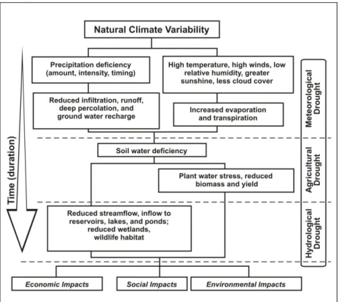
1.6.2. Drought definitions
Drought is a continued period of anomalous dry weather having a great impact in causing problems in agriculture, animal production and / or water supply. Figure 10 explains the evolution of drought with the time.
Figure 10 - Drought definitions (National Drought Mitigation Center)
1.6.3. Meteorological drought
The meteorological drought is a measure of the deviation of precipitation in relation to the normal value, characterized by water shortages induced by the imbalance between precipitation and evaporation, which depends on other factors such as wind speed, air temperature and humidity, insolation. The definition of dry weather must be considered depending on the region, since the atmospheric conditions that result in deficiencies of precipitation can be very different from region to region.
1.6.4. Agriculture drought
The agricultural drought is associated with water shortages caused by the imbalance between the available soil water, the need of crops and plant transpiration. This type
therefore being associated with drought crop characteristics, the natural vegetation, or agricultural systems in general.
1.6.5. Hydrological drought
The hydrological drought is related to the median reduction of water in the reservoir and the soil’s water depletion. This type of drought occurs after the meteorological and agriculture drought, since a longer time is required for the precipitation deficiencies to manifest themselves in various components of water systems.
1.6.6. Socio-economic drought
The socio-economic drought is associated with the combined effect of natural and social impacts that result from water shortage, due to the imbalance between the supply and demand of water resources affecting directly populations.
1.6.7. Drought estimation
The amount and distribution of annual rainfall, and high values of air temperature, are conditions that determine the intensity and consequences of a drought. In order to estimate the possibility of a drought, or its severity, one must know the weather conditions.
Meteorological data that are more important to know are, for example, the precipitation, air temperature, air humidity and water content in the soil.
The effects of droughts can be immediately felt in agriculture, because it is directly dependent of the water storage in soil, where other activities may only be subsequently affected since they can depend on superficial reserves. Generally, the activities that depend on groundwater reserves are the last to be affected. When normal conditions are restored, the water replacement is done in reverse: first the water reserves in the soil, followed by the flow of watercourses and reservoirs and lakes and finally groundwater. The recovery time is dependent on the duration and severity of dry and precipitation checked after it’s finished.
1.6.8. Standard Precipitation Index (SPI)
The SPI (Standard Precipitation Index) is an index developed by Mckee, Doesken, & Kleist (1993) in order to set and monitoring local droughts and it was designed also to identify droughts in different timescales. Although it has been designed to identify drought periods it can also be used in the identification of humid periods. The analyzed scales are usually monthly (SPI-1 month) and seasonal or trimestral (SPI, 3 months), although also calculate annual SPI (SPI-12 months). Different timescales reflect the delay in the
response of different resources water anomalies of precipitation. As the time scale increases, SPI response becomes slower to precipitation changes.
The SPI is calculated based on the probability distribution of rainfall for the period chosen. Thus, the SPI index values obtained depend on the distribution function chosen from the sample values from which the parameters are determined from the distribution, and also the estimation method. The SPI allows comparisons between different locations and different periods of time due to the fact that this index indicates the distance between the observed precipitation and average for a given month, and also be normalized by the standard deviation of the precipitation site of the month.
The SPI calculated in this way has the following characteristics (Mckee, Doesken, & Kleist, 1993)
SPI is uniquely related to the probability;
Precipitation used in the SPI can be used to calculate the deficit precipitation for the period used;
Precipitation used in the SPI can be used to calculate the current percentage of the average rainfall for the time period k months;
SPI is normally distributed and therefore can be used to monitoring dry periods as humid periods;
SPI is normalized, so dry and wet periods are represented in similar ways.
1.6.9. Palmer Drought Standard Index (PDSI)
The PDSI is a meteorological drought index, and it responds to weather conditions that have been unusually dry or unusually wet. When conditions change from dry to normal or wet, for example the drought measured by the PDSI ends without taking into account streamflow, lake and reservoir levels, and other longer-term hydrologic impacts (Karl & Knight, 1985). The PDSI is calculated based on precipitation and temperature data, as well as the local Available Water Content – AWC – of the soil. From the inputs, all the basic terms of water balance equation can be determined, including evapotranspiration, soil recharge, runoff and moisture loss from the surface. Human impacts on the water balance, such as irrigation, are not considerate.
1.7. Cultural coefficient (K
c)
According to Doorenbos & Pruitt (1977), a crop evapotranspiration (ETc) can be calculated from the reference evapotranspiration (ETo) and crop coefficient (Kc) at different growth stages. ETo is the evapotranspiration of a hypothetical culture, actively growing, without limitation water and expresses the evaporating power of the atmosphere at a specific
temporal and spatial scale, without considering the characteristics of the soil and crop. Allen, Pereira, Raes, & Smith, (1998) recommended the use of the Penman-Monteith equation with some simplifications, also known as the FAO Penman-Monteith method as the standard method for estimating the ETo from climatic data.
The crop coefficient (Kc) is experimentally obtained relationship between ETc and ETo, and represents the integration of the effects of four characteristics that distinguish the crop evapotranspiration of reference evapotranspiration: the height of culture, the resistance of the canopy, the albedo of the soil surface cultivation, and water evaporation on the soil surface (Pereira & Allen, Novas aproximações aos coeficientes culturais, 1997).
2. METHODS
2.1. Study area
Portugal is located in southwestern Europe, on the Iberian Peninsula, between latitudes 37º and 42º N, in the transitional climatic region between the sub-tropical anticyclone and the sub-polar depression zones. Portugal's climate is Mediterranean, with strong north-south and west-east climatic variability. Mean annual temperature values vary between 7ºC in the inner highlands of central Portugal and 18º C in the southern coastal region. Mean monthly air temperature values have a distinct pattern during the year, reaching their maximum in August and minimum in January. Mean annual precipitation in mainland Portugal is around 900 mm, with the highest values (above 3000 mm) in the highlands of the northwest region and the lowest values (around 500 mm) in the southern coast and in the eastern part of the territory (below or around 500 mm). On average, about 42% of annual precipitation falls during the 3-month winter season (December-February) and the lowest values occur during summer (June-August), corresponding to only 6% of annual precipitation, as it is characteristic of Mediterranean climates. (Rego, Acácio, Van Lanen, & Stahl, 2013)
2.1.1. Dataset
We selected the meteorological stations with the longest and most complete dataset of monthly precipitation across a north-south gradient in Portugal. Precipitation data was obtained from the Portuguese Meteorological Service (Institute of Meteorology). Characteristics of the selected meteorological stations and the precipitation dataset are provided in Table 4.
Gauging stations (table 5) with monthly streamflow data were selected based on the following simultaneous criteria:
Proximity to one of the selected meteorological stations (maximum distance: approximately 100 km);
Near-natural streamflow (disturbances as low as possible during the period of time selected), with no overt adjustment of “natural” streamflow, such as flow diversion or augmentation, regulation of the streamflow by some flow-reducing structure (e.g. dam or weir), or reduction of base flow by extreme groundwater pumping;
Catchment area not too large (< 1000 km2);
Long and complete time series of recorded monthly streamflow (minimum 30 years and no more than 10% of values missing during the period of record).
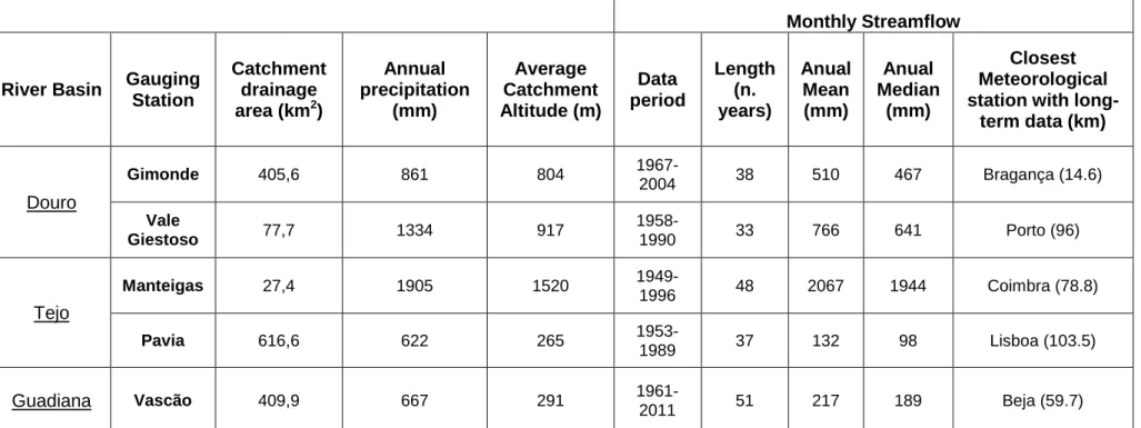
These were compared with metadata on regulation and catchment area from the national streamflow database (table 6) - the National Information System on Hydric Resources (SNIRH), a public dataset provided by the Portuguese Water Institute (INAG/APA). The quality and length of the data series was highly variable and most of the 416 stations had short-term or incomplete data series and regulation. An initial group of 32 gauging stations was selected to go through quality control, including detection of visible inhomogeneities or mislabelled missing values (e.g. zeros). After a final quality check, five stations were selected for analysis (table 4). The selected stations cover a north-south climatic gradient in mainland Portugal (table 4). Stations located in Douro basin, northern Portugal, show higher streamflow values than stations located in Tejo and Guadiana basins, southern Portugal. Streamflow is higher than precipitation (2067 and 1905 mm, respectively) for the pair of meteorological-gauging stations Coimbra–Manteigas because the catchment drained by the Manteigas gauging station is at higher altitude than the Coimbra rain gauge. A more nearby rain gauge at the same altitude than the Manteigas gauging station with sufficient long record was not available. For each station, monthly volumetric discharge (L3, dam3) was transformed into monthly streamflow (mm) by dividing the volumetric discharge by the catchments area (L2, km2).
Watershed characterization
Monthly Streamflow
River Basin Gauging Station Catchment drainage area (km2) Annual precipitation (mm) Average Catchment Altitude (m) Data period Length (n. years) Anual Mean (mm) Anual Median (mm) Closest Meteorological station with
long-term data (km) Douro Gimonde 405,6 861 804 1967-2004 38 510 467 Bragança (14.6) Vale Giestoso 77,7 1334 917 1958-1990 33 766 641 Porto (96) Tejo Manteigas 27,4 1905 1520 1949-1996 48 2067 1944 Coimbra (78.8) Pavia 616,6 622 265 1953-1989 37 132 98 Lisboa (103.5) Guadiana Vascão 409,9 667 291 1961-2011 51 217 189 Beja (59.7) Table 4 - Characterization of selected meteorological stations and precipitation dataset
Meteorological Station Latitude (ºN) Longitude (ºW) Altitude (m) Available Data period Mean Annual Precipitation (mm) Annual Precipitation Standard Deviation (mm) Bragança 41° 48´ 6° 44´ 690 1945-2011 708 199 Porto 41° 08´ 8° 36´ 93 1864-2011 1209 307 Coimbra 40° 12´ 8° 25´ 141 1866-2011 946 215 Lisboa 38° 43´ 9° 09´ 77 1864-2011 720 197 Beja 38° 01´ 7° 52´ 246 1941-2011 543 171
Table 5 - Characterization of selected gauging stations and streamflow dataset
Gauging Station Own drained area (km2) Average altitude of drained area (m) Average slope Average number of flows Maximum retention Total annual rainfall (mm) Gimonde 405,6 803,66 0,159 77,082 32,835 861 Vale Giestoso 77,722 916,85 0,112 76,207 34,479 1334 Manteigas 27,405 1519,49 0,329 86,118 17,802 1905 Pavia 616,634 264,76 0,055 78,849 29,623 622 Vascão 409,894 291,03 0,106 73,677 39,456 667
stations. The latitude of gauging stations ranges from 38° 01´ (Gimonde, Bragança) to 41° 48´ (Vascão, Beja).
Figure 11 - Location of selected catchments and meteorological stations (Rego, Acácio, Van Lanen, & Stahl, 2013)