$:AstonBusinessSchool,UniversityofAston,Birmingham,B47ET,UK$$:UniversidadeCat Âolica Portuguesa,Porto,Portugal
School Outcomes: Sharing the Responsibility
Between Pupil and School
1EMMANUEL THANASSOULIS$and MARIA DA CONCEI ÄAO A. SILVA PORTELA$$
ABSTRACT This paper uses a Data Envelopment Analysis based approach to decompose pupil under-attainment into that attributable to the school the pupil attends and that attributable to the pupil. The approach measures pupil attainment in terms of value added. Data on over 6700 A-level pupils from 122 English schools have been analysed. The results suggest that at current levels of school effectiveness a pupil’s own application accounts for the major part of any under-attainment, though schools also have scope to improve their effectiveness. The approach also makes it possible to identify target attainment levels a pupil could be set and the extent to which the attainment of those targets necessitates an improvement in the effectiveness of the school the pupil attends and in the pupil’s own efforts.
Introduction
Assessments of school effectiveness have hitherto largely focusedon school level comparisons.Typically theyhave useddataoncontextualvariablesto estimatean expectedlevelofattainmentonexitfromaschool’spupils.Thecomparisonofthis estimatewithitsobservedcounterpart givesameasureoftheschool’seffectiveness. Themethodofchoiceforobtainingtheestimatesofexpectedattainmenthasbeen regression analysis [e.g. see Jesson (1992), Gray et al. (1986), Sammons et al. (1996)].Whendataatpupillevelexistmulti-level modelling canbeusedtoestimate expectedoutcomesatdifferenthierarchicallevels.Typicallypupilsaretakenaslevel 1,cohorts(classes)aslevel2,schoolsaslevel3andsoon.Multi-levelmodellingis a regression-based method that makes it possibleto decomposethe variation of pupilattainmentintoproportions attributabletoeachlevelofdata,(pupils,classes, schoolsetc.).Moredetailsonmulti-levelmodellinganditsuseineducationcanbe found in Goldstein (1987, 1995, and 1997), O’ Donoghue et al. (1997), and Sammonset al. (1993).
This paper uses the linear-programming-based method of Data Envelopment Analysis (DEA)applied topupilleveldata todecomposepupilandschooleffects on pupil attainment. DEA, developed by Charnes et al. (1978), is a
general-purpose method for assessing performance and has seen application to `units of assessment’ such as bank branches, retail outlets, hospitals and regulated utilities. The interested reader can find introductions to DEA in Charnes et al. (1994), Cooper et al. (2000), Boussofiane et al. (1991) and Thanassoulis (2001). DEA-based but school level assessments can be found in Smith and Mayston (1987), Jesson et al. (1987), Bessent et al. (1982), Mayston and Jesson, (1988), FÈare et al. (1989), Thanassoulis (1996a, b) and Thanassoulis and Dunstan (1994). The use of pupil-level data in DEA assessments is quite recent, having started, to the authors’ knowledge, with the work of Thanassoulis (1999). The advantages of using pupil-level data in studying value-added in education are well rehearsed, (e.g. see O’Donoghue et al., 1997, Goldstein 1997) in terms of multi-level modeling being more efficient than OLS regression in providing information about the relative performance of institutions and of students of varying academic ability. We use in this paper DEA at pupil level with the specific aim of decomposing pupil-level under-attainment into respective components attribut-able to the pupil and the school attended. Such information, it is argued, can help focus effort where it would be most effective in improving pupil attainments.
Value added at pupil level is assessed in this paper by comparing pupil attainments after allowing for contextual variables which have an impact on those attainments. The basic aim of the paper is to ascertain the relative impact of pupils and schools on the attainment of pupils and to illustrate additional insights gained into pupil and school performance by decomposing school and pupil impacts on pupil attainment. The data used relates to 6700 pupils aged 18, attending a random sample of 122 schools and so the results offer a fair indication of the scale of school and pupil effects on pupil performance at national level in England. Separation of school and pupil effects is very important if the root causes of good and poor performance are to be identified and dealt with. The separation of the impacts makes it additionally possible to identify differential school effectiveness so that a school may alter any bias in its effectiveness to the benefit of all its pupils. Finally, the approach also makes it possible to set targets for pupils with indications as to the component of the targets that should be attainable by the pupil given his/her school’s effectiveness, and the component that the pupil can only attain if his/her school improves its effectiveness.
The terms efficiency and effectiveness are used in overlapping senses in this paper. Efficiency measures will be defined later in precise quantitative terms in relation to the maximum exit attainments a pupil might have been expected to reach, given his or her attainments on entry to the schooling stage being assessed. In contrast, we refer to an effective school or pupil as one respectively fostering or attaining best exit outcomes but we do not define or use precise measures of effectiveness.
DEA differs from multi-level modelling applied to pupil level data in four important ways:
d In DEA there is no need to specify a functional form linking pupil attainment and hypothesised `explanatory’ factors;
d Random noise in pupil attainment is allowed for in DEA in a subjective manner without making assumptions about its statistical properties;
d DEA can handle multiple explanatory and multiple `dependent’ (attainment) variables so that the multi-outcome nature of the education process can be modelled more accurately. (Handling multiple outputs in a regression context though feasible in principle is far less straightforward.)
d DEA is a `frontier’ or `boundary’ method so that maximum rather than average outcomes are estimated for given contextual (explanatory ) values.
These features give certain advantages to the DEA-based approach of this paper over multi-level modelling, at the expense of not according statistical noise inherent in pupil attainment a formal statistical treatment. We do, however, allow for such noise in a simpler way where certain exceptionally good outcomes by pupils are adjusted downwards before being used as benchmarks for judging the performance of other pupils. This leads to erring on the side of conservative estimates of the degree of pupil, and thereby school, under-attainment on exit. The DEA-based approach used in the paper can therefore be applied either as an instrument of pupil and school assessment in its own right or to complement multi-level modelling studies, dropping for example single-outcome and/or functional specifications used, and exploring boundary rather than average behaviour.
The paper is laid out as follows. The next section (section 2) presents a graphical illustration of the method used for decomposing pupil and school impacts on pupil attainment. Section 3 applies the method to a set of real data. Section 4 discusses the insights gained through the decomposition of pupil under-attainment and section 5 concludes.
A Graphical Illustration of the DEA Approach for Decomposing Pupi l Efficiencies
The approach used in this paper to decompose pupil under-attainment into school and pupil effects was also used in Portela and Thanassoulis (2001) to decompose school and school-type impacts on pupil attainments, school-type relating to funding regime of the school. It is inspired by that used by Charnes et al. (1981), to decompose school efficiencies into managerial and policy efficiencies. The approach in this paper differs, however, from that of Charnes et al. (1981), in that we use pupil level rather than aggregate school level data and we decompose only radial measures of efficiency.
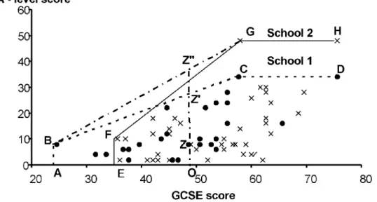
In order to illustrate graphically this approach for decomposing pupil and school impacts on pupil attainment we shall assume that we have data on two variables for two British secondary schools, labelled school 1 and school 2. One variable reflects pupil attainment on exit, the pupil’s A-level score, and the other reflects pupil attainment on entry, the pupil’s GCSE score. We shall compare pupils on attainment on exit reflected in their A-level score, controlling for their innate ability proxied by their GCSE score. (For those unfamiliar with the British educational system, A-level [General Certificate of Education Advanced Level] examinations are normally taken by pupils at age 18, typically preceded by GCSE [General Certificate of Secondary Education] examinations at the age of 16.) A fuller discussion of the actual choice of contextual factors and attainment variables used in this paper follows later.
Figure 1 shows fictitious data for schools 1 and 2. Each pupil is represented by a dot in the case of school 1 and a cross in the case of school 2. Since we are controlling for innate pupil ability (proxied by the GCSE score) any variation in the exit attainment (A-level score) of the pupils will be the result of:
d random noise (reflecting also omitted variables);
d differences in effectiveness between the two schools and; d differences in application by pupils.
The piece-wise linear boundary ABCD in Figure 1 corresponds to school 1 and that of EFGH to school 2. We refer to such boundaries as `pupil-within-school boundary’ . When, on the other hand, we consider all the pupils in Figure 1, irrespective of the school attended, the piece-wise linear boundary ABGH is referred to as the `pupil-within-all-schools boundary’ . These frontiers are based on DEA under variable returns to scale (VRS) (Banker et al., 1984) and represent maximum exit attainments observed or estimated for given entry attainments. The segments BA, FE, GH, and CD are boundary but not efficient as they are dominated by B, F, G, and C, respectively. Elsewhere boundary points are efficient in that exit attainments are maximum for the corresponding GCSE score, that maximum not being feasible for a lower GCSE score within the comparative set of pupils considered (single school or multi-school as the case may be).
The pupils enveloped by some frontier are inefficient relative to that frontier. We shall define now two measures of radial DEA-efficiency of pupil Z attending school 1 in Figure 1, using respectively the within-all-schools and pupil-within-school boundaries. A third measure of efficiency, relating to the school rather than the pupil, will then be defined using the pupil-related measures of efficiency.
Pupil-Within-All-Schools Efficiency Measure
The pupil-within-all-schools boundary is ABGH. The radial distance of pupil Z from this boundary is measured by the ratio
OZ OZ 0
where Z0 represents the within-all-schools maximum output (i.e. A-level score) pupil Z could have attained, given its input level (i.e. GCSE score).
The ratio OZ
OZ 0 is the pupil-within-all-schools DEA-efficiency rating of
pupil Z.
The pupil-within-all-schools efficiency of pupil Z reflects the proportion of A-level score the pupil is achieving relative to the best he/she could have achieved as estimated with reference to pupils of all (i.e. both in this case) schools considered, and given his/her GCSE score on entry. We ignore at this stage random noise on attainment levels recorded, but will come to it later. In the single output context used here it is not readily apparent why the measure of efficiency
OZ OZ 0
is radial. As can be seen in model (M1) in Appendix 1 where we deal with multiple outputs, the efficiency measures used are radial because they relate to estimates of maximum attainable levels on all output variables when they are raised by the same factor.
Pupil-Within-School Efficiency Measure
The pupil-within-school boundary of school 1 is ABCD. The radial distance of pupil Z from his/her within-school boundary is
OZ OZ 9
where Z9 represents the within-school maximum output (i.e. A-level score) pupil Z could have attained, given its input level (i.e. GCSE score).
The ratio OZ
OZ 9 is the pupil-within-school DEA-efficiency rating of
pupil Z.
The pupil-within-school efficiency of pupil Z reflects the proportion of A-level score the pupil is achieving relative to the best he/she could achieve as estimated with reference to pupils of his/her own school (i.e. school 1) and given his/her GCSE score on entry. (We ignore again at this stage noise on attainment levels recorded.) School effects are absent from the ratio
OZ OZ 9
as we are comparing pupils attending the same school. Therefore the distance of pupil Z from the boundary (point Z9) is attributed to the pupil’s effort as the school
has demonstrated, through the achievements of other pupils, that point Z9 represents a feasible attainment level at the school, for the GCSE score of pupil Z. By way of qualification of this statement we note that random noise on pupil attainment has been ignored up to this point as has the possibility that a school may purposely focus its efforts on a subset of its pupils and thereby artificially show under-attainment by the remaining pupils as a pupil rather than school effect. The possibility of such school behaviour is addressed ex post under `differential school effectiveness’ later in this paper.
School-Within-All-Schools Efficiency Measure
Unlike the previous two efficiency measures which are pupil-specific, this measure relates to the distance between the pupil-within-school and pupil-within-all schools boundaries at the input level(s) of a pupil. Thus the measure is not dependent on the attainment of the pupil whose input level(s) specify the point where the distance of the two boundaries is measured. The distance between the pupil within-school and within-all-schools boundaries at the input level of pupil Z in Figure 1 is
OZ 9 OZ 0
The ratio OZ 9
OZ 0 is the school-within-all-schools DEA-efficiency rating at the
input level of pupil Z.
This measure reflects the component of the under-attainment of pupil Z which cannot be attributed to pupil Z, but rather to the school the pupil attends. To see this, note that if pupil Z had attained the maximum A-level score for his/her GCSE score she/he would have been at point Z9. Then, the pupil-within-all-schools-efficiency of pupil Z would have been
OZ 9 OZ 0 As OZ 9
OZ 0 < 1
there is some inefficiency. This inefficiency cannot be attributed to the pupil as she/ he is attaining the best-observed performance in his/her own school for his/her attainment on entry. This inefficiency is thus attributed to the school pupil Z attends.
Looking now at the three DEA-efficiencies defined so far we have the following decomposition of the overall measure of under-attainment
OZ OZ 0 of pupil Z:
OZ OZ 0 = OZ OZ 9
´
OZ 9 OZ 0 (1)That is, the global measure of under-attainment
OZ OZ 0
of pupil Z, is the product of two measures of under-attainment. The measure OZ
OZ 9
attributable to the pupil’s own efforts, and the measure OZ 9
OZ 0
attributable to the school the pupil attends.
The approach outlined so far can be used to decompose efficiency at as many levels as desired in the same manner as variance in pupil attainment can be decomposed by means of multi-level modelling at any number of hierarchical levels. We have applied the decomposition to two-levels here but see Portela and Thanassoulis (2001) for a three-level decomposition of pupil-within-all-schools efficiency.
Decomposing Pupil Efficiencies in a Large Random Sample of English Secondary Schools
The two main stages in effecting the decomposition in expression (1) are the identification of contextual and outcome variables to measure value added, and the computation of the DEA-efficiency measures needed.
Choice of Contextual and Outcome Variables
Contextual variables are intended to allow for factors not controllable by pupil or school but affecting pupil attainment so that value-added may be captured. There is an extensive body of literature as to exogenous factors influencing pupil attainment. Most of the existing studies, however, concern pupils in the age group 11± 16 [see for example Gray et al. (1986), Gray et al. (1990), Sammons et al. (1993 and 1996) Mayston and Jesson (1988), and Jesson et al. (1987)], and only a few concern A-level studies [Fitz-Gibbon (1985), Fitz-Gibbon (1991), Tymms (1992), and O’Donoghue et al. (1997)].
It is generally agreed that attainment on entry is one of the most important factors explaining pupil attainments on exit. Another variable generally considered important is the socio-economic background of the pupil. The surrogate variable
used for this in England is normally the pupil’s eligibility for free school meals or, less often, his/her parents’ occupation(s). Socio-economic background was found, however, more important in pre-A-level rather than in A-level attainment. (See for example Fitz-Gibbon, (1985; 1991); and Tymms, (1992)). This is perhaps explained by the fact that pre-A-level study is compulsory while A-level studies are optional. There is thus a degree of self-selection on socio-economic factors in post age 16 education in England. Finally, there is no strong evidence that gender and ethnicity influence attainment at A-level, (Fitz-Gibbon, 1991, and Tymms, 1992) though they have been found to have some impact in pre-A-level attainment. O’Donoghue et al. (1997) have found some statistical significance in the relationship between attainment at A-level and gender. They also analysed the relationship between attainment and age, concluding that this was a small effect not contributing much to explaining the progress of A-level students.
Drawing on the foregoing research we selected the contextual and outcome variables in Table 1 to measure value added to pupil attainment at A-level.
The two contextual variables in Table 1 are proxies for the innate ability of the pupil. GCSEpts reflects the total number of subjects attempted at GCSE and the grades obtained. (Conversion rates are given in Table 2.) This variable will fail to reflect innate ability of pupils who attempt a small number of subjects at GCSE. (This could be because their school did not support some subjects.) The GCSE points per attempt will reflect pupil ability where the pupil attempts only a few subjects but achieves good grades. To be precise, our input variables capture academic performance rather than innate ability and the strength of correlation between the two may vary across schools. In the general case, our approach here can be used with the best variables available on innate ability. For the analysis at hand, the GCSE results were the best proxy on innate ability at our disposal as they do explain by far the largest variation in pupil A-level attainment. (O’Donoghue et al., 1997; Fitz-Gibbon, 1985, 1991; and Tymms, 1992).
The outcome variables in Table 1 reflect pupil attainment on exit from A-level studies. The first variable rewards the breadth of subjects taken, permitting trade-offs between the number of subjects taken and the grade attained in each subject. The second outcome variable rewards high attainment per subject attempted, even if the subjects attempted were few. Typically exit academic results of this kind are
Table 1. Outcome and contextual variables for value added at A-Level Contextual variables (inputs) Outcome variables (outputs)
d Total GCSE points (GCSEpts) d Total A and AS points (Apts)
d GCSE points per attempt (GCSEpts_att) d A and AS points per attempt (Apts_att)
Table 2. Grade and corresponding score points
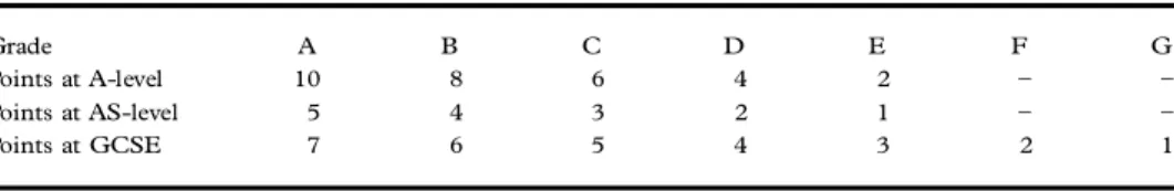
Grade A B C D E F G
Points at A-level 10 8 6 4 2 ± ±
Points at AS-level 5 4 3 2 1 ± ±
used by researchers in this area because they are readily available and objectively measured. It is, however, generally recognized that the academic results reflect only one of the multiple outcomes of education. See, for example Gray (1981), and Thanassoulis and Dunstan (1994) for broader views on the outcomes of education.
In the context of the DEA approach the contextual variables are inputs and the outcome variables outputs and we have used an output oriented assessment in the sense that we wish to measure maximum attainable output levels controlling for input levels.
Computation of the DEA efficiencies Needed for Decomposing Pupil Under-Attainment
The Department for Education and Employment (DfEE) of the UK provided us with (anonymized) data of all pupils taking A and AS level examinations in 1994 in a random sample of 122 schools in England. The data covered over 6700 pupils. We had data on GCSE and A-level attempts and results for each pupil. The GCSE, A-level and AS level grades were converted to points using the scales in Table 2.
Using the contextual and outcome variables in Table 1 we computed, with reference to each pupil j0in our sample the two efficiency measures, denoted EFFwj0
and EFFij0, where EFFwj0is the pupil-within-school and EFFij0is the
pupil-within-all-schools DEA efficiency of the pupil. The technical details of the computation of the foregoing two efficiencies can be found in Appendix 1. These two efficiency measures were then used to compute the school-within-all-schools DEA efficiency EFFsj0at the input levels of pupil j0, where
EFFsj0 =
EFFij0
EFFwj0
(2)
Letter grade numerical correspondences of the type shown in Table 2 are used widely by schools, government, universities and others in the UK and provide de facto a numerically based system for measuring the contextual and outcome variables in Table 1. (GCSE letter grades now also include A* typically set to numerical 8.) However, each original letter grade reflects banding of a range of original performance levels and the numerical grades derived from the letter grades will generally reflect differently the ratios of the original performance levels, depending on how we convert letter grades to numerical values. Thus, our efficiency results depend on the particular letter to numerical values conversion scale we use. Appendix 1 details how the efficiencies computed can change if we change the numerical letter grade correspondences. The efficiencies therefore need to be interpreted within the context of the specific letter-grade numerical corre-spondences used within the DEA model.
Dealing with Random Noise in Pupil Attainment
In practice, pupil attainments both at exit and on entry will incorporate random noise. Random noise in input variables would mean that we control
incorrectly for the context of a pupil’s attainment on exit, especially so far as reflecting their innate ability is concerned. Random noise on exit attainment could mean that we estimate incorrectly the A-level attainments feasible in principle for a given set of values of the input variables. Random noise in output attainments could also reflect the impact of omitted contextual variables on attainments on exit.
Our approach to dealing with random noise focuses on mitigating its impact on estimates of pupil under-attainment and on the constituent components of pupil-within-school and school-within-all-schools components. This was done by adjusting downwards the attainment of exceptional pupils. The procedure used for this purpose was based on that developed in Thanassoulis (1999) and technical details of how it was used here can be found in Appendix 1.
The impact of adjusting downwards the attainment of exceptional pupils is that we shift closer to the student body (by a subjectively determined amount) the within-school and the within-all-schools efficient boundaries depicted in Figure 1. Thus we make a conservative estimate of what pupils within a school are capable of attaining at best in A-levels on exit and the same goes across the system of all schools considered, controlling for pupil context. This adjustment can also have an impact on our estimate of the school-within-all-schools efficiencies depending on the relative shift we introduce to the within-school and within-all-schools boundaries when allowing for random noise. Crucially, the estimate of school-within-all-schools efficiency at the level of inputs of a particular pupil is not affected by any random noise in the attainment levels of that particular pupil, unless that random noise has an impact on the positioning of the within-school or within-all-schools efficient boundaries. The reader can readily verify this by noting that for example in the context of Figure 1, the school-within-all-schools efficiency measure
OZ 9 OZ 0
is independent of the position of pupil Z along the vertical line OZ 9 so long as the pupil does not have an impact on the location of any boundary.
So far as random noise in the input variables is concerned, if for any given pupil we have an incorrect estimate of their innate ability then our approach will estimate the attainment they might have reached at A-level for the innate ability their GCSE levels reflect but which may under or over estimate their true innate ability. This means our results ought to be used with caution at pupil level, as a guide to what a pupil may be capable of rather than prescriptively. However, when the pupil level results are aggregated to school level to estimate for example average within-school or within-all-schools efficiencies of pupils then random noise in input levels is mitigated by virtue of the fact that it is two-sided, over-estimating innate abilities of some and under-estimating those of others. The mitigation is better the larger the number of pupils at the school.
Clearly the results we derive after allowing for random noise on pupil attainment are sensitive to the subjective thresholds we use in deciding what pupils are to be treated as exceptional (see Appendix A). One way to mitigate the impact of this in real life policy making contexts is to carry out sensitivity analysis to gauge the degree of sensitivity of the results obtained to the subjective thresholds used. We did not
undertake this further analysis in the illustration of our method reported in this paper.
Results
Our results are summarized in Table 3. More extensive results at school level can be found in Appendix 2.
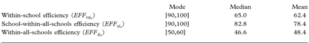
Looking at the median within-all-schools efficiency of 46.6% we find that half the pupils assessed attain at A-level less than 46.6% of the A-level points and points per A-level attempted that their best counter parts attain after we control for GCSE attainments on entry but NOT for school attended. This is remarkably poor attainment, considering that we have discounted already anything up to 10% of the better performing pupils as exceptional (see Appendix 1) so as to make a conservative estimate of best attainment feasible within, and by extension, across schools, controlling for input levels. The next issue is to what extent can this within-all-schools under-attainment at A-level be blamed on the school attended or on the pupil’s application.
The within-school efficiencies of pupils have a median of 65%. So when we control both for GCSE grades AND for school attended still half the pupils only attain at A-level less than 65% of the scores they could be expected to attain. This suggests that much of the pupil under-attainment at A-level is the result of lack of pupil application rather than school effectiveness. Our analysis supports better this statement at the school rather than pupil level since, as noted earlier, random noise impacts are mitigated when the results are looked at school level. However, as also noted earlier, low pupil-within-school efficiencies may be indicative of the school focusing its efforts on only a subset of its pupils, leading to relatively low pupil-within-school efficiencies for the rest of the school’s pupils. We cannot in such a circumstance attribute low pupil-within-school efficiencies solely to the lack of application by the school’s pupils. We can, however, as we will see later under differential school effectiveness, identify cases where schools may be only effective with a subset of their pupils, if that subset has a common feature, such as having good attainments on entry.
The median school-within-all-schools efficiency in Table 3 is just under 83%. Thus there is scope for schools to improve their own effectiveness to take pupils to still higher attainments than those they currently secure even when they are `top’ attaining pupils at the schools. Thus both pupils and schools have to do work to improve pupil attainment but most gain will come from pupils at least reaching best attainment within their own school.
The summary results of Table 3 can of course hide the varying picture at school level. The next section outlines some further insights gained on pupil and school performance through the within-all-schools efficiency decomposition.
Table 3. Measures calculated at pupil-level across all pupils (122 schools)
Mode Median Mean
Within-school efficiency (EFFwj0) ]90,100] 65.0 62.4
School-within-all-schools efficiency (EFFsj0) ]90,100] 82.8 78.4
Insights Gained Through Decomposing Pupil Under-attainmen t A More Precise Allocation of Responsibilities for Improving Pupil Attainment
As argued in the preceding section, the divergence between within-school and within-all-schools DEA-efficiencies, reflected in school-within-all-schools effi-ciencies, captures the impact of a school on pupil attainment. The use of the decomposed efficiencies is illustrated in Figure 2.
Figure 2 shows the within-all-schools and within-school efficiency scores at pupil level in two schools, identified as school 60 and school 121. The distance between the two efficiency measures is much larger at school 60 than at school 121, where the two efficiency measures coincide for the vast majority of pupils. It can be seen in Appendix 2 that within-school and within-all-schools efficiencies average respectively 82.40% and 48.80% at school 60. The corresponding figures for school 121 are 56.45% and 52.01%. Thus at both schools the pupils attain a similar average proportion of the A-level grades we would expect from a within-all-schools perspective, that is about 50% in round figures. Yet, in school 121 pupils lie a similar average distance from the within-all-schools and the within-school boundary which means that some of its pupils are good enough to be on the within-all-schools boundary which raises the within-school to the within-all-within-all-schools boundary. In contrast, in school 60 the average distance of pupils from the within-school boundary is over 33 percentage points shorter than their average distance from the within-all-schools boundary. Thus most pupils are relatively close to the within-school boundary but hardly any are good enough to be on the within-all-schools boundary which means the two boundaries are generally far apart. The fact that in the case of school 60 the within-school and within-all-schools boundaries are further apart than is the case for school 121 is evident in Figure 2 from the distances between the diamond and star symbols represent-ing respectively the within-school and within-all-schools efficiencies of each pupil.
We have identified that there is scope for pupils both at school 60 and at school 121 to reduce their average distance from the within-all-schools boundary by a similar amount, which approximates to doubling the output levels (A-level outcomes) they currently attain, controlling for input levels (GCSE innate ability proxies). However, in the case of school 60 most of the effort must come from the school itself since the pupils are relatively close to their within-school boundary (they attain on average 82.4% of the best in the school) while in the case of school 121 most of the effort must come from pupils since they attain only just over half (56.45%) of what the best in the school attain. These different components pupils and schools 60 and 121 can contribute in closing roughly the same `overall’ average efficiency gap of pupils at both schools is reflected in the different mean school-within-all-schools efficiencies of the two schools. It can be seen in Appendix A2 that school 121 has mean school-within-all-schools effi-ciency of 93.8% while that of school 60 is 60.56%. So school 60 needs to improve its effectiveness more than school 121. This, of course, does raise the additional question as to why school 121 is effective with a subset of pupils who reach the within-all-schools boundary but not with the bulk of its pupils. As we will see next, there is evidence that school 121 is differentially effective, focusing on the most able of its pupils.
Identifying Differential School Effectiveness
We shall refer to a school as being differentially effective when it does not facilitate with uniform effectiveness the attainments of all of its pupils. This could be as a result of a deliberate policy focusing on raising the attainments of a subset of pupils, (e.g. teaching to stretch the more able pupils while not stretching to their full Fig. 2. Within-school (©) and within-all-schools (*) efficiencies at schools 60
potential the less able pupils) or the result of other events such as using relatively inexperienced teachers with some subsets of pupils or otherwise varying teaching practices across groups of pupils. In cases of differential school effectiveness the attribution of pupil-within-school efficiency to the pupil and of school-within-all-schools efficiency to the school is not totally valid and needs to be used with caution in a school management context.
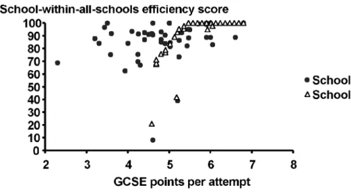
Once we have decomposed pupil-within-all-schools efficiencies as outlined earlier we can attempt to detect differential school effectiveness at school level. This will be easier when differential effectiveness relates to pre-defined groups of pupils, such as those based on attainment at entry. Figure 3 illustrates the approach.
The school-within-all-schools efficiency scores of schools 121 and 2 are plotted in Figure 3 against the GCSE points per attempt of each pupil in the school. The graph suggests that school 121 is more effective with those of its pupils who offer higher attainment scores on entry. In contrast, there is no pattern to school-within-all-schools efficiencies in the case of school 2 and so no evidence of differential effectiveness, at least not with reference to attainment of pupils on entry. Note incidentally that Figure 3 also suggests that pupils in school 121 have, in general, higher attainment on entry than those of school 2, as measured by GCSE points per attempt. Further, school 121 does better than school 2 with pupils of higher attainment but worse than school 2 with some of the weakest on entry! This is strongly suggestive of school 121 not catering well for its weakest on entry pupils. The graphical approach sketched above can be complemented or indeed replaced by a numerical approach to identify evidence of differential school effectiveness. For example we could compute the mean, median and other summary statistics of school-with-all-schools efficiencies for pupils grouped by attainment on entry to A-level studies. Thereby we can detect any evidence of differential school effectiveness. For example in the case of schools 121 and 2 in Figure 3 we have the results in Table 4.
The fact that school 121 appears to be more effective with the top half of its cohort on entry (those who offer above the median GCSE points per attempt) than with the bottom half is borne out by the summary statistics in the first two
numerical columns of Table 4. Some 75% of the top half on entry are found at input levels where school-within-all-schools efficiency is 100% when the corresponding efficiency is as low as 78.72% for the bottom half of the school cohort (see Q1 figures). This difference between the two halves of the school cohort of over 21 percentage points in school-related efficiency drops to about 5 percentage points when we get to median school-within-all-schools efficiency (100± 94.99). The difference is nevertheless statistically significant (Mann± Whitney test). The two halves of the school cohort cease to differ on school-within-all-schools efficiency once we get to the top 25% (see Q3 figures) on school-within-all-schools efficiency. In contrast, looking at the numerical columns under school 2 the median and Q3 school-within-all-schools efficiencies within each half of the school cohort are quite close and not indicative of differential effectiveness. Only at the Q1 level of school-within-all-schools efficiencies is there some evidence that school 2 is more effective with the top half on entry.
Summary statistics of this type on school-within-all-schools efficiencies can help find indications of differential school effectiveness be it on attainment on entry, on socio-economic background or on any other criterion for grouping pupils. If differential school effectiveness exists but does not relate to any readily identifiable group of pupils it will prove harder to detect.
Identifying Role Model Pupils and Setting Attainment Targets
The disentangling of school from pupil impacts on performance makes it possible to set pupils targets of achievement which can incorporate separate components for improvements in pupil and school efficiency. The role model pupils that a pupil can emulate to attain his/her targets are also identified. Target A-levels must be set, of course, prior to the A-level examinations. The outcomes of `mock’ A-level examinations taken some six or so months before the A-level examinations proper could provide the outputs needed in the context of the efficiency decomposition procedure outlined here.
Table 4. School-within-all-schools efficiencies (%) by pupils grouped on GCSE points per attempt
School 121 Bottom 50% on entry* Top 50% on entry** School 2 Bottom 50% on entry* Top 50% on entry** Min 20.83 95.01 8.22 39.09 Q1 78.72 100.00 75.35 84.61 Median 94.99 100.00 90.60 88.82 Mean 84.93 99.87 82.32 88.04 Q3 100.00 100.00 92.12 95.99 Max 100.00 100.00 100.00 100.00
* Pupils offering below the median GCSE points per attempt, the median relating only to pupils of the school concerned.
** Pupils offering above the median GCSE points per attempt, the median relating only to pupils of the school concerned
An approach for target setting is detailed in Thanassoulis (1999) for pre-A-level pupils and this can be readily adapted to the pre-A-level stage of education being analysed here. The A-level targets for pupil j0flow directly from the model used to assess DEA efficiencies and can be found in expressions (A1) and (A2) in Appendix 1. Appendix 1 also details the identification of the role model pupils pupil j0 could emulate to improve his/her performance. These are DEA-efficient pupils who offer on the contextual variables a very similar profile to that of pupil j0. This makes it possible to hold out the efficient peers as role models for pupil j0to emulate.
By construction of the efficiency assessment model, the targets reflect the maximum radial expansion feasible to the attainments of pupil j0, followed by further improvement where possible to one of the two A-level attainment measures used in the model. Depending on the comparative set of pupils used in the assessment model the targets will reflect expectations on a within-school or a within-all-schools basis.
Targets based on the within-school efficient frontier should be attainable by the pupil even if his/her school was merely to retain its current effectiveness, unless the school has differential effectiveness to the detriment of the pupil concerned. The targets remedy the shortfall in the pupil’s performance relative to that of other pupils in his/her school who have the same attainment on entry. The efficient peer or role model pupils in this case will be exclusively drawn from the pupil’s own school.
Targets based on the within-all-schools efficient frontier reflect the A-level attainments a pupil might be expected to reach to match the best pupils of his/her innate ability (as proxied by the GCSE attainment measures used) anywhere within the set of schools from which pupils have been drawn. These targets can only be more demanding than those based on the within-school efficient frontier. If the all-schools targets are indeed more demanding than the within-school targets then the pupil concerned can only attain them if his/her within-school were to become as effective for pupils of his/her GCSE attainments on entry as the schools from which the pupil’s within-all-schools efficient peer pupils are drawn.
Impacts on Pupil Attainment Beyond those due to Pupil and School Effectiveness
We can use the approach outlined so far to ascertain the impact on pupil attainment by pupil groupings below school level. For example A-level pupils belong to different groups by subject taken. Fitz-Gibbon (1991) notes that classes (teaching units) within-schools can be as different as different schools. Thus our assessment as outlined above will fail to reflect class or teaching unit impacts on pupil performance within a given school. Instead, since we put together all pupils of a school, the within-school targets and DEA-efficiencies will reflect the best performance that can be expected in any class of the school, after discounting attainments of exceptional pupils (see Appendix 1). This may not be reflective of the attainment pupils taught in less effective classes (teaching units) of the school can reach. Given relevant data, especially for schools with many classes, within-school efficiencies should be estimated after inserting an intermediate level to assess within class (teaching unit) efficiencies. This extension of our approach is relatively simple but is not illustrated here. We could not ascertain school-class or teaching unit level impacts on pupil attainment because our data were not
detailed enough. However, our data did allow us to decompose efficiencies at three levels, pupil, school and type of school (in terms of funding regime). The results of this three-level decomposition can be found in Portela and Thanassoulis (2001).
Conclusion
This paper has used an approach for estimating the part of the under-attainment of a pupil which is attributable to his/her own application as distinct from the part attributable to the school the pupil attends. The approach is based on DEA, increasingly used as a main stream method of performance measurement in all sectors of the economy. The adaptation presented here requires data on contextual and outcome variables at pupil level. Such data are used to estimate the maximum outcome levels that can be expected from a pupil given the levels she/he has on the contextual variables. By grouping pupils hierarchically at school and then at within-all-schools level we can estimate the components of any under-attainment by a pupil on the outcome variables which can be attributed to the pupil and to the school the pupil attends.
Using the method we analysed data on over 6700 A-level pupils from 122 English schools. The results suggest that there is scope for pupils to improve a great deal on attainment, even when we discount attainment levels reached by exceptional pupils. Further, both schools and pupils can contribute to improving pupil attainment but the larger component can come from the pupils’ own application, to reach the best attaining pupils within their school, controlling for prior attainment. The approach also makes it possible to identify differential school effectiveness across particular groups of pupils and to set target attain-ments at pupil level. The targets incorporate a separate component which the pupil should be capable of attaining given the effectiveness of the school she/he attends, and a further component the pupil may attain if the effectiveness of his/ her school improves. The method can also be used, although our own data did not permit it, to ascertain the impact of pupil grouping below school level (e.g. at school class level) on pupil attainments.
Information of the kind yielded by the decomposition method presented here should be of value both to current and prospective pupils of the school. It should also be of value to teachers of the school as well as to those running it.
Notes
1. The authors are grateful to the Leverhulme Trust for financial support with this research and to the UK Department for Education and Employment for providing data. The contents of the paper are the responsibility of the authors and no representation is being made that they are shared by those funding or collaborating with this research.
References
Andersen, P. and Petersen, N. (1993) A Procedure for Ranking Efficient Units in Data Envelopment Analysis, Management Science, 39, 1261± 1264.
Banker, R. D., Charnes, A., and Cooper, W. W. (1984) Some models for estimating technical and scale inefficiencies in Data Envelopment Analysis, Management Science, 30, 1078± 1092. Banker, R. D. and Morey, R. C. (1986) Efficiency Analysis for Exogenously Fixed Inputs and
Bessent, A., Bessent, W., Kennington, J., and Reagen, B. (1982) An Application of Mathematical Programming to Assess Productivity in The Houston Independent School District, Management
Science, 28, 1355± 1367.
Boussofiane, A., Dyson, R. G., and Thanassoulis, E. (1991) Applied Data Envelopment Analysis,
European Journal of Operational Research, 52, 1± 15.
Charnes, A., Cooper, W. W., and Rhodes, E. (1978) Measuring Efficiency of Decision Making Units, European Journal of Operational Research, 2, 429± 444.
Charnes, A., Cooper, W. W., and Rhodes, E. (1981) Evaluating program and Managerial Efficiency: An Application of Data Envelopment Analysis to Program Follow Through,
Management Science, 27, 668± 697.
Charnes, A., Cooper, W. W., Lewin, Y. A., and Seiford, M. L. (Eds) (1994) Data Envelopment
Analysis: Theory, Methodology and Application, Kluwer Academic Publishers, (Boston, Dordrecht,
London)
Cooper, W. W., L. M. Seiford and K. Tone, (2000) Data Envelopment Analysis: A comprehensive text
with models, applications, references and DEA-solver software. (Kluwer Academic Publishers
(Boston, Dordrecht, London).)
Dusansky, R. and Wilson, P. W. (1994) Technical Efficiency in the Decentralized Care of the Developmentally Disabled, Review of Economics and Statistics, 76, 340± 345.
FÈare, R., Grosskopf, S., and Weber, W. L. (1989) Measuring School District Performance, Public
Finance Quarterly, 17/4, 409± 428.
Fitz-Gibbon, C. T. (1985) A-levels Results in Comprehensive Schools: the COMBSE project. Year 1, Oxford Review of Education, 11, 43± 58.
Fitz-Gibbon, C. T. (1991) Multi-level Modelling in an Indicator System, in: S. W. Raudeubusch and J. D. Willms (Eds) Schools, Classrooms, and Pupils, International Studies of Schooling from a
Multilevel Perspective, Academic Press, San Diego. Chapter 6, 67± 83.
Goldstein H. (1987) Multi-level Models in Educational and Social Research, Charles Griffin and Co, London, Oxford University press, New York.
Goldstein H. (1995) Multi-level Statistical Models, (2nd edition) London, Edward Arnold. Goldstein, H. (1997) Methods in school effectiveness research, School Effectiveness and School
Improvement, 8, 369± 395.
Gray, J. (1981) A Competitive Edge: examination results and the probable limits of secondary school effectiveness, Educational Review, 33, 25± 35.
Gray, J., Jesson, D., and Jones B. (1986) The Search for a fairer way of comparing schools’ examination results, Research Papers in Education, 1, 91± 122.
Gray, J., Jesson, D., and Sime, N. (1990) Estimating differences in the examination performance of secondary schools in six LEAs: a multi-level approach to school effectiveness, Oxford Review
of Education, 16, 137± 158.
Jesson, D., Mayston, D., and Smith, P. (1987) Performance Assessment in the education sector: educational and economic perspectives, Oxford Review of Education, 13, 249± 266.
Jesson D. (1992) Beyond the league tables, Education, 179/9, 179± 180
Mayston, D., and Jesson, D. (1988) Developing Models of Educational Accountability, Oxford
Review of Education, 14, 321± 339.
O’Donoghue, C., Thomas, S., Goldstein, H., Knight, T. (1997) 1996 DfEE study of Value Added for 16± 18 years olds in England, DfEE Research Series, RS52, March 1997
Portela, M. C. S. and Thanassoulis E. (2001) Decomposing school and school type efficiencies,
European Journal of Operational Research, 132/2, 357± 373.
Sammons, P., Nuttall, D., and Cuttance, P. (1993) Differential school effectiveness: results from a re-analysis of the Inner London Education Authority’s Junior School Project Data, British
Educational Research Journal, 19, 381± 405.
Sammons, P., Thomas Motimore, P., Owen, C., and Pennell, H. (1996) Assessing School Effectiveness:
Developing measures to put school performance in context, OFSTED, Publications Centre, London.
Smith, P. and Mayston, D. J. (1987) Measuring Efficiency in the Public Sector, OMEGA-the
international Journal of Management Science, 15, 243± 257.
Thanassoulis E. and R. G. Dyson, (1992) Estimating preferred input output levels using data envelopment analysis. European Journal of Operational Research, 56, 80± 97.
Thanassoulis E., and Dunstan, P. (1994) Guiding Schools to Improved Performance Using Data Envelopment Analysis: An Illustration with Data from a Local Education Authority, Jour nal of
the Operational Research Society, 45, 1247± 1262.
Thanassoulis E. (1996a) Altering the bias in differential school effectiveness using data envelopment analysis, Journal of the Operational Research Society, 47/7, 882± 894.
Thanassoulis, E. (1996b) Assessing the Effectiveness of Schools with pupils of different ability using Data Envelopment Analysis, Journal of the Operational Research Society, 47/1, 84± 97. Thanassoulis, E. (1999) Setting Achievement Targets for School Children, Education Economics,
7/2, 101± 119.
Thanassoulis, E. (2001) Introduction to the Theory and Application of Data Envelopment Analysis: A
foundation text with integrated software. Kluwer Academic Publishers, Boston.
Tymms, P. B. (1992) The Relative Effectiveness of Post-16 Institutions in England (Including Assisted Places Schemes Schools), British Educational Research Journal, 18, 175± 192.
Wilson, P. W. (1995) Detecting Influential Observations in Data Envelopment Analysis, The
Journal of Productivity Analysis, 6, 27± 45.
Appendix 1. Computational Details of the Decomposition of Pupil Under-Attainment Between School and Pupil Effects
The decomposition of school and pupil effects on pupil attainment requires the computation of the pupil-within-school and pupil-within-all-schools DEA effi-ciencies. The generic DEA model used is the same for computing both efficiencies but the set of comparative pupils differs in each case. Before we define the comparative set of pupils for each efficiency measure, let us assume that it consists of n pupils. Then using the input-output variables in Table 1, the output oriented radial DEA-efficiency of pupil j0relative to that set of pupils is:
100 Q*j0%
where Q*j0is the optimal value of Q in the following model:
Max
lj,SGCSEPts.SGCSEpts_att,SApts,SApts_att.Q
Q
S.t. Sn
j = 1GCSEptsjlj + SGCSEPts = GCSEptsj0
Sn
j = 1GCSEpts_attjlj + SGCSEpts_att = GCSEpts_attj0 (M1)
S
n
j = 1Aptsjlj± SApts = Q Aptsj0
S
n
j = 1Apts_attjlj± SApts_att = Q Apts_attj0
Sn
j = 1lj = 1
ljj = 1, . . ., n, SGCSEPts, SGCSEpts_att, SApts, SApts_att ³ 0,
Q free
GCSEPts, GCSEpts_att, Apts and Apts_att are as defined in Table 1, j subscripting the pupil. The model attempts to estimate the maximum feasible radial expansion, Q of the A-level attainments of pupil j0given his/her GCSE attainments. The measure of efficiency is radial because it relates to raising all outputs by the same expansion factor Q.
The generic model on which model (M1) is based is that developed by Banker and Morey (1986), for the case of assessing DEA-efficiencies under variable returns to scale (VRS), where certain inputs are exogenously fixed. Both inputs in our case are exogenously fixed. The Banker and Morey (1986) model would use a non-Archimedean infinitesimal « to give, in the objective function of (M1) second priority to the maximization of the output slack variables SApts and SApts_att after first maximising Q. We carry out this second order maximisation of slack variables in a separate model (M2) below.
In the educational context measurement scales of attainments are arbitrary. Therefore, there is no reason to expect that if the GCSE attainments of two pupils represent some scaling to each other, then if both pupils are `efficient’ , their A-level attainments will be related by the same scaling factor. This makes our assumption of VRS appropriate. In the practical context addressed in this paper, the levels of the inputs are fixed in the sense that they represent recorded pupil attainments (GCSE grades) at the commencement of the schooling period to which the efficiency assessments relate. This leads us to adopt an output orientation in model (M1) (and (M2) later) to estimate the potential for output augmentation at pupil j0.
As noted earlier, the letter grade numerical correspondences of the type depicted in Table 2, used within model (M1), are used widely in the UK but the results of model M1 are sensitive to the particular scale used. Specifically, given that (M1) is output-oriented the efficiency measures derived will be unaffected if we simply translate the input data by adding some numerical constant (assuming the input data remain non-negative). (See Cooper et al. (2000), section 4.3.2 on translation invariance under VRS.) If not only the input, but also the output data are translated by the addition of an arbitrary constant, the efficiency rating of pupils will generally change but the classification of pupils into efficient and inefficient will not change. (This is readily deduced from Theorem 4.6 in Cooper et al. 2000.)
The comparative sets of pupils n for computing within-school and within-all-schools DEA-efficiencies were derived as follows.
Within-school DEA-Efficiencies .
The comparative set of pupils consists of the pupils of the school except that we discount part of the A-level attainment of certain of its pupils, to whom we shall refer as exceptional pupils. This is done to allow for random noise on pupil attainment and is carried out using a procedure originally developed in Thanassou-lis (1999). This procedure rests on the idea that if a sufficiently large proportion of the pupils of a school reach a certain level of attainment on exit when we control for their attainments on entry, then that level of attainment on exit is genuinely feasible within that school relative to the attainments on entry concerned. What constitutes a sufficiently large proportion of the pupils of the school in this context is subjective. For example we will run a higher risk of incorrectly concluding a certain attainment level at exit is genuinely feasible at a school, controlling for contextual variables, if only 10% rather than 15% of the pupils of the school reach it. On the other hand the higher this proportion the higher the risk that we will under-estimate the best level that is genuinely attainable by pupils on exit, controlling for context.
To identify the pupils to be treated as exceptional in the foregoing context, we first computed the super-efficiency (Andersen and Petersen 1993) for each pupil within his/her own school. A pupil was now deemed potentially exceptional if he/she achieved outcome levels which were at least 20% higher than we would expect for
his/her input levels, based on all pupils of the school except for the pupil being tested for exceptionality and those already identified as exceptional. (Computational details can be found in Thanassoulis 1999.) Next we used the approaches in Wilson (1995) and Dusansky and Wilson (1994) to filter as exceptional only those of the pupils of a school who not only had super-efficiency above 120% but were also influential in being efficient peer of many other pupils and affecting substantially the efficiencies of many other pupils. Subjective thresholds were used in all these procedures treating no more than 10% of the pupils of a school as exceptional. As noted earlier the robustness of the results obtained would normally need to be tested against the subjective thresholds used here but this was not carried out as our results are illustrative rather than an input to managerial action on schools.
The exceptional pupils identified in the foregoing manner had their A-level attainments scaled radially down to render each one of them 100% efficient within model (M1) when the set of comparative pupils is that of the non-exceptional pupils. This approach is consistent with discounting a component of the A-level attainment of exceptional pupils as not indicating school effectiveness but rather stochastic impacts (random noise). Note also that our interest in random noise in the context of this procedure is one-sided, concerned only with the possibility of artificially raising rather than lowering the levels of efficient attainment.
The comparative set for computing the within-school radial DEA-efficiencies of the pupils of a school consists of the pooled set of its non-exceptional and of its non-exceptional pupils after the A-level attainments of the latter group have been scaled down as detailed above.
Note that we have not allowed for noise on the attainment of non-exceptional pupils. A non-exceptional pupil might have achieved more than would be `normal’ within their school for their level of application and attainment on entry, or the reverse. Thus our estimate of the within-school efficiency of a pupil may contain an error component. This error averaged across all pupils of the school should be low but at pupil level it could be high. Thus, we should use our pupil-level results for guidance rather than prescription as to what the pupil may be capable of attaining.
The procedure outlined above is applied to each school in turn and terminates with a set of pupils used to compute the within-school radial DEA-efficiencies of the pupils of that school.
Within-All-Schools DEA-Efficiencies
The comparative set of pupils for computing the within-all-schools radial DEA-efficiencies of pupils is constructed by pooling together all pupils of all schools. Exceptional pupils are used at their lower (discounted as above) levels of attainment.
As in the case of within-school efficiencies, within-all-schools efficiencies at pupil level too contain an error term due to random impacts on pupil attainment. Note, however, that within-school and within-all-schools boundaries were constructed so as to reflect what might be attainable by best performing pupils, after allowing for exceptional pupil attainment. Thus school-within-all-schools efficiencies that
measure the distance between these two boundaries should suffer less from random noise since the two boundaries are drawn conservatively, after discounting some of the outlier pupil performances in terms of high attainment.
With reference to Figure 1, when model (M1) is used to compute the within-school efficiency of pupil Z it would yield
Q*j0 = OZ9 OZ
and for his/her within-all-schools efficiency it would yield
Q*j0 =
OZ0 OZ
wherever Z9 and Z0 lie after any pupils at either school have had their A-level attainments `reduced’ by reason of being exceptional in the foregoing context.
Targets of Attainment on Exi t
In the practical context addressed in this paper, the levels of the inputs are the recorded attainments (GCSE grades) of pupil j0 at the commencement of the schooling period to which the efficiency assessments relate. Hence, targets can only relate to exit grades pupil j0might attain. Such targets can be set prior to the exit stage A-level examinations, using as a basis say A-level results from mock A-level examinations taken some months prior to the A-level examinations proper. Let n be a set of comparative pupils, drawn from one or more schools as data permit. Exceptional pupils are identified and treated as outlined in respect of model (M1) above which is then solved. Let the optimal value of Q be Q*j0. Solve
now model (M2). Max
lj,SGCSEpts.SGCSEpts_att,SApts,SApts_att SApts + SApts_att
S.t. S
n
j = 1GCSEptsjlj + SGCSEPts = GCSEptsj0
S
n
j = 1GCSEpts_attjlj + SGCSEpts_att = GCSEpts_att j0 (M2)
Sn
j = 1Aptsjlj± SApts = Q*j0Apts j0
Sn
j = 1Apts_attjlj± SApts_att = Q*j0Apts_att j0
Sn
j = 1lj = 1
ljj = 1, . . ., n, SGCSEPts, SGCSEpts_att, SApts, SApts_att ³ 0 We use the same mock A-level (or other suitable) data in model (M2) as in (M1). GCSEPts, GCSEpts_att, Apts and Apts_att are as defined in Table 1, the j subscript
the pupil. The target levels of A-level points and A-level points per attempt for pupil j0 within the set of comparative pupils being used are respectively TAptsj0 and TApts_attj0, where TAptsj0 = S n j=1Aptsjlj* (A1) TApts_attj0 = S n j=1Apts_attjlj* (A2)
and the superscript * denotes optimal values of the corresponding variables in model (M2).
In model (M2) we are estimating additional potential increases to the A-level points and A-level points per attempt of pupil j0 that might have been feasible beyond the radial expansion of these two outputs by the factor Q*j0computed in
model (M1). The input slack variables SGCSEPts and SGCSEpts_att do not feature in the objective function of model (M2) because the corresponding input levels are `fixed’ . (See the underlying generic model in Banker and Morey 1986.) Where the values of both slack variables SGCSEPts and SGCSEpts_att are not zero at the optimal solution to (M2) pupil j0should be able to reach the targets in (A1) and (A2) even if his/her GCSE attainments had been lower by the amounts reflected in those slack variables. In this context, the values of input slack variables are treated as simply informational.
It should be noted that in fact the targets estimated for a pupil need not be unique. In principle targets can be estimated to reflect a variety of priorities the pupil, school and/or parents may attach to the different measures of attainment. The appropriate models for this purpose are beyond the scope of this paper but can be found in Thanassoulis and Dyson (1992) or Thanassoulis (2001).
With reference to Figure 1, (if we assume A-level results are from mock examinations), model (M2) will yield targets with respect to pupil Z at Z9 and Z0 when the comparative set of pupils is the within-school and within-all-schools respectively, wherever Z9 and Z0 lie after any exceptional pupils at either school have had their A-level attainments `reduced’ as above. The slack values both in the input and in the output related constraints will be zero. Model (M2) will only yield a non-zero output slack in the context of Figure 1 when the pupil lies on a vertical segment of the boundary such as AB or EF taking the target output attainment to point B or F respectively. A non-zero slack in the input constraint will only be identified when the pupil lies on a horizontal segment such as GH or CD. In such a case, however, the target output attainment remains on the horizontal segment as it is identical with that of the `dominating’ point G or C which used lower GCSE attainment grades.
Efficient Peers to an Inefficient Pupi l
Let superscript * denote optimal values of the corresponding variables in model (M2). The DEA peers to pupil j0are pupils j for whom lj* is positive at the optimal
solution to (M2). As can be seen in (A1) and (A2) the target level for pupil j0on each A-level attainment measure is based exclusively on the attainments of his/her efficient peers on that measure.