ORE RESERVE ESTIMATION USING RADIAL BASIS FUNCTIONS
Jorge Kazuo YAMAMOTO RESUMO
Este trabalho apresenta uma aplicação das equações multiquádricas para o cálcu-lo de reservas minerais. Esse método é comparado com os estimadores tradicionais usados na indústria mineral: inverso da distância e krigagem ordinária. A função de base radial com um termo de precisão constante tem uma forma absolutamente equiva-lente à krigagem ordinária. Nesse sentido, as funções de base radial podem ser poten-cialmente empregadas para avaliação de reservas minerais. Além disso, as funções de base radial podem ser adaptadas facilmente para avaliação de blocos tal como a krigagem. É mostrado também que as funções de base radial são dependentes das unidades das coordenadas e, dessa forma, as funções base devem ser cuidadosamente escolhidas. Usando os dados exploratórios do Depósito de Cobre de Chapada, demonstra-se que a transformação logarítmica das funções base proporciona os melhores resultados quan-do comparaquan-dos aos da krigagem ordinária. Assim, as funções de base radial podem ser aplicadas para estimativa de reservas minerais, tornando-se uma alternativa confiável para essa finalidade.
Palavras-chave: inverso da distância, krigagem ordinária, função de base radial, avaliação de reservas minerais, Depósito de Cobre de Chapada.
ABSTRACT
This paper presents an application of multiquadric equations for ore reserve estimation. This method is compared with available traditional estimators used in the mining industry: inverse distance weighting and ordinary kriging. Radial basis function with a constant precision term has a dual form absolutely equivalent to the ordinary kriging. In this sense, radial basis functions present a potential application for ore reserve estimation. Besides, radial basis functions can be adapted easily to allow block estimates as block kriging does. It is shown that radial basis functions depend on the metrics of data coordinates and so the basis functions should be carefully chosen. This paper also discusses kernel transformation for improving radial basis function estimates. Using the exploration data from the Chapada Copper Deposit, it is shown that logarithmic transformation of basis functions provides the best results comparable to the ordinary kriging ones. Thus, radial basis functions can be applied for ore reserve estimation, becoming a reliable alternative to this task.
Keywords: inverse distance weighting, ordinary kriging, radial basis function, and ore reserve estimation, Chapada copper deposit.
1 INTRODUCTION
Approximation of a variable at unsampled points is a common procedure used for computer aided ore reserve estimation. Usually, a mineral deposit is discretized in small blocks of dimensions compatible with the available exploration data. The discretization is made within recognized boundaries
defined by the exploration data. A certain number of blocks have to be estimated and their individual ore reserves determined. The estimation or interpolation procedure is applied to determine the reserve parameters for a block using neighboring exploration data. There are basically two interpolation methods that have been used for computer aided ore reserve estimation: inverse distance weighting and ordinary
kriging. The first method is indicated when available data do not justify variogram computation and so the ordinary kriging technique cannot be applied. The second one has been used extensively by the mining industry for ore reserve estimation. However, it is important to mention that interpolation for three-dimensional data is not limited to these methods. There are several available methods that could be applied for ore reserve estimation. One of these methods is derived from radial basis functions, which allows approximation of any irregular surface by means of a sum of a number of kernel surfaces. Radial basis functions are a generalization of multiquadric equations, which were firstly suggested by R.L. Hardy for the analytical representation of a terrain surface from discrete data points (HARDY, 1971). Although radial basis functions have been developed for interpolation of two-dimensional data, it can be extended for three-dimensional data as well as for higher dimensions. This paper presents an application of radial basis functions for ore reserve estimation.
2 ORE RESERVE ESTIMATION METHODS
As introduced before the current methods for ore reserve estimation are: inverse distance weighting and ordinary kriging.
The inverse distance weighting was among the first computer-based techniques used in ore deposit calculations (PHILIP & WATSON, 1987). Kriging is the standard name given to the collection of generalized linear regression techniques for minimizing an estimation variance defined from a prior covariance model (OLEA, 1991). There are many different types of kriging methods depending on objectives, conditions and constraints for each type. So, kriging with a known mean receives the name of simple kriging (SK), kriging for the mean value receives the name of kriging of the mean (KM), kriging with an estimated mean receives the name of ordinary kriging (OK), among other types of available kriging methods. Details for these different types of kriging can be found in (WACKERNAGEL, 1995). In this paper only the ordinary kriging will be considered because its formulation allows solving most of the ore reserve estimation problems.
2.1 Inverse distance weighting
The inverse distance weighting is an interpolation technique for estimating values of
locationally dependent variables by forming a linear combination of a set of measurements (PHILIP & WATSON, 1987). The non-negative weights sum up to one and are inversely related to the distance to data points (PHILIP & WATSON, 1987). The grade or any other variable at unsampled points can be estimated by using the inverse distance weighting as:
⎪
⎪
⎪
⎩
⎪⎪
⎪
⎨
⎧
=
=
=
≠
=
∑
∑
= =0
*
'
,
1
0
1
.
1
*
' 1 ' 1 i i i n i p i n i i p id
if
F
F
n
i
for
d
if
d
F
d
F
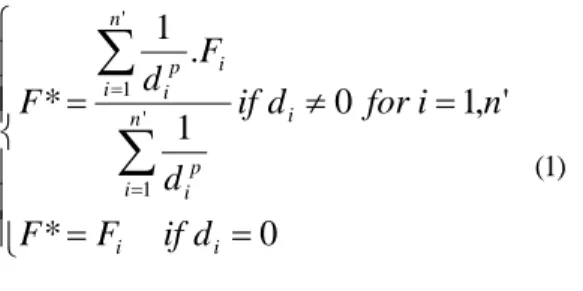
(1)where di is the distance from each of the n’ sample locations to the point to be estimated, p is the power of distance, and F1, ..., Fn’ are the grade values. Therefore, the normalized weight for the i-th sample becomes:
∑
==
n' j p j p i id
d
W
11
1
(2) SAMPLE 3 SAMPLE 4 SAMPLE 1 SAMPLE 2FIGURE 1 - Block estimation by extending the grade computed in its center.
For ore reserve estimation this technique was used for interpolating a point in the center of an evaluation block (Figure 1). The resulting grade was extended to the whole block with an associated error proportional to the block size.
This author (YAMAMOTO, 1996) has proposed a new method of block calculation using the inverse distance weighting method, according to the following equation:
i ' n i i
.
F
W
.
*
F
∑
==
1 (3)where
W
i is the average of the inverse distance weighting of the i-th sample in relation to all sub-blocks. This new method is an adaptation of the conventional block kriging method, where a block estimate is equal to the average of point estimatescentered on sub-blocks. So, given a block it is discretized into nsb sub-blocks of equal size. For block discretization the limits given by JOURNEL & HUIJBREGTS (1978) are recommended (Table 1).
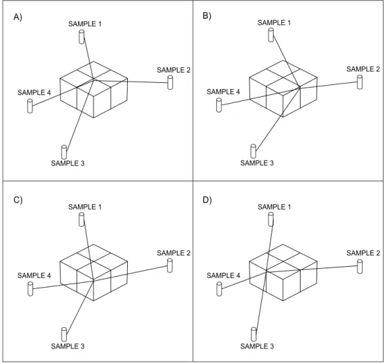
Normalized weights between samples and each sub-block are computed as illustrated in Figure 2.
The normalized weight between i-th sample and k-th sub-block is:
TABLE 1 - Discretization limits for the discrete approximation of a block (after JOURNEL & HUIJBREGTS, 1978).
domain dimension number of points
One 10 Two 6 x 6 Three 4 x 4 x 4 A) SAMPLE 3 SAMPLE 4 SAMPLE 1 SAMPLE 2 B) SAMPLE 3 SAMPLE 4 SAMPLE 1 SAMPLE 2 C) SAMPLE 3 SAMPLE 4 SAMPLE 1 SAMPLE 2 D) SAMPLE 3 SAMPLE 4 SAMPLE 1 SAMPLE 2
FIGURE 2 - Computation of normalized weights for each sub-block: A) for the sub-block 1; B) for the sub-block 2; C) for the sub-block 3; D) for the sub-block 4.
∑
==
n' j p k , j p k , i k , id
d
W
11
1
(4)After the normalized weights for all sub-blocks have been computed, the average weight for each sample is computed as follows:
∑
==
nsb k k , i iW
nsb
W
11
, for i=1 to n’ (5)where nsb is the number of sub-blocks.
Expression (5) allows computing the grade of a block directly as does ordinary kriging. Obviously, it gives the same result as the average of grades of nsb sub-blocks. However, the great advantage of expression (5) is the direct calculation of an estimation error of inverse distance weighting block estimates, by means of the interpolation variance as proposed by this author (YAMAMOTO, 2000) for ordinary kriging estimates. The interpolation variance of a block can be computed as:
(
)
∑
= ∗−
=
n i i i oW
F
F
S
1 2 2Actually, this is an extension of the same formula used for computing a measure of the reliability of ordinary kriging estimates. This extension is valid for inverse distance weighting because their weights are positive and are normalized, which assures the positiveness of the interpolation variance.
2.2 Ordinary kriging
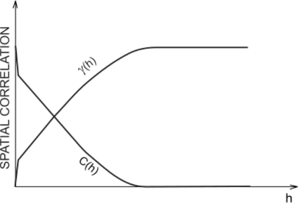
Kriging depends firstly on a structural function C(h) or γ(h), which describes the spatial correlation of data points (Figure 3).
Ordinary kriging (OK) is the most widely used kriging method and is based on local second-order stationarity (JOURNEL & HUIJBREGTS, 1978). Ordinary kriging is by excellence the recommended method for ore reserve estimation, because it was designed for block evaluation. Indeed, ordinary kriging was the first method that provided block
computation.
OK estimate is based on weighted average of available data:
( )
∑
( )
==
n' i i i o.
F
x
x
*
F
1λ
(6)where the weights {λi, i=1,n’} are determined by the solution of a kriging system of equations.
In order to ensure unbiasedness of estimates, the expected value of the error
[
( ) ( )
o o]
* x F x F − is set to zero:
( ) ( )
{
F
x
F
x
}
,
E
* o−
o=
0
which can be developed as:
( )
{
( )
o}
' n i i iF
x
E
F
x
E
=
⎭
⎬
⎫
⎩
⎨
⎧
∑
=1λ
( )
{
}
{
( )
}
∑
==
' n i o i iE
F
x
E
F
x
1λ
since E
{
F( )
xi}
=m and E{
F( )
xo}
=m then(7) C(h) h SP A T IAL CORRELA TION g(h)
FIGURE 3 - Typical variogram and correspondent covariance.
which is known as the non-bias condition (JOURNEL & HUIJBREGTS, 1978).
On the other hand, ordinary kriging makes estimation under the condition that the error variance is minimum. The error variance is:
( )
( )
{
o o}
OK
=
Var
F
x
−
F
*
x
2
σ
(8)which can be written after ISAAKS & SRIVASTAVA (1989) as:
( ) ( )
{
}
( ) ( )
{
}
( ) ( )
{
o o}
o o o o OKx
F
x
F
Cov
x
F
x
F
Cov
x
F
x
F
Cov
*
*
*
2
2+
−
=
σ
(9)Deriving each term on the right side of (9), we have:
( ) ( )
{
}
{
( )
}
( )
0 C x F Var x F x F Cov o o o = = ( ) ( ){
}
( ) ( ) ( ) ( ) ( ) { ( )} ( ) ( ) { } { ( )} { ( )} ( ) ( ) { } { ( )} { ( )} [ ] (o i) i i i o i o i i i i o i i o i i o i i i o i i i o i i i o o x x C x F E x F E x F x F E x F E x F E x F x F E x F E x F E x F x F E x F x F Cov x F x F Cov − = − = − = ⎭ ⎬ ⎫ ⎩ ⎨ ⎧ − ⎭ ⎬ ⎫ ⎩ ⎨ ⎧ = ⎭ ⎬ ⎫ ⎩ ⎨ ⎧ ⎥ ⎦ ⎤ ⎢ ⎣ ⎡ = ∑ ∑ ∑ ∑ ∑ ∑ ∑ ∗ λ λ λ λ λ λ λ 2 2 2 2 2 2 2 2( ) ( )
{
}
{
( )
}
( )
(
)
∑∑
∑
− = ⎭ ⎬ ⎫ ⎩ ⎨ ⎧ = = ∗ ∗ ∗ i j j i j i i i i o o o x x C x F Var x F Var x F x F Cov λ λ λThus, expression (9) becomes:
( )
−∑
(
−)
+∑∑
(
−)
= i i j j i j i i o i OK C λC x x λλCx x σ2 0 2Minimization of the error variance (10) constrained to the unbiasedness condition (7) results in the following system of ordinary kriging equations:
(
)
(
)
⎪ ⎩ ⎪ ⎨ ⎧ = = − = + −∑
∑
1 1 j j i o i j j jC x x C x x ,for i ,n λ µ λ (10)where µ is the Lagrange multiplier.
In the case of block kriging the right side:
(
x
ox
i)
C
−
of the ordinary kriging system (10) is replaced byC
(
x
o−
x
i)
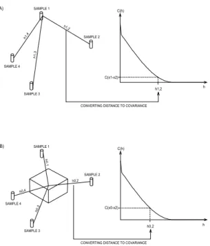
, i.e. the average covariance between the i-th point and centers of sub-blocks.Figure 4 illustrates the process of converting distances to covariances. Figure 4A shows how to compute the covariances between sample 1 and all others. Repeating this process for all samples we will take into account the mutual dependence among samples. This feature recognizes spatial clusters and assigns correct weights to the samples. In Figure 4B distances between samples and the center of the block are converted to covariances (point kriging).
The set of weights {λi, i=1,n’} results from the solution of the ordinary kriging system (10). These weights applied to expression (6) give the estimated value. The error associated with the estimated value is given by:
( )
∑
(
)
= − − − = n' i i o i OK C .C x x 1 2 0 λ µ σ (11)See that the kriging variance is homoscedastic, i.e. it is independent of the data used to obtain the estimator F*(xo) (OLEA, 1991). Figure 5 illustrates why kriging variance should not be used as an approximation of uncertainty (ARMSTRONG, 1994). As the data layouts are identical in both cases, the kriging variances are identical and as it happens, so are the kriged estimates (ARMSTRONG, 1994).
3 RADIAL BASIS FUNCTIONS
Radial basis functions are a generalization of the original multiquadric equations (HARDY, 1971). The basic hypothesis of the multiquadric analysis is that any smooth mathematical surface, and also any smooth arbitrary surface (mathematically undefined) may be approximated to any desired degree of exactness by the summation of a wide variety of regular, mathematically defined surfaces, particularly quadric forms (HARDY, 1977). The quadric forms are not only the simplest, but also the most efficient
in converging on irregular surfaces (HARDY, 1977). Now, the quadric forms are in fact one of the available kernels of radial basis functions. It is important to mention that although radial basis functions were defined on global basis, local approximation can give reliable results. In this regard, accuracy of multiquadrics can be improved and computational effort can be dramatically reduced by transforming a large global problem into many small quase-local problems by domain decomposition (KANSA, 1990). A radial basis function with centers in {x1,x2,. . . ,xn’} as given in BEATSON & NEWSAM (1992) is represented as:
( )
∑
(
)
=−
=
n' i o i i oc
.
x
x
x
*
F
1φ
(12)where n’ is the number of neighboring points and f is a symmetric radial function in Rn. Indeed, this is the form originally proposed by HARDY (1971), but a more general form has been proposed by other authors (CARLSON & FOLEY 1992, GIROSI 1992, MYERS 1992), which includes a second summation for equation (12) as:
( )
∑
(
)
∑
( )
= =+
−
=
k j j j ' n i o i i oc
.
x
x
a
.
p
x
x
*
F
0 1φ
where pj(x), j=0,..,k are the polynomial terms in the position coordinates of x. Solution for this system of equations requires the following set of constraints:
( )
x
,
j
,
,
k
p
c
' n i j i0
0
K
1=
=
∑
=Addition of polynomial terms does not mean a precision improvement, because it may degrade the accuracy of the interpolant on some data sets (CARLSON & FOLEY, 1992). Thus, some authors (MICCHELLI 1986, MADYCH 1992) have used the expression (12) with just a term of degree 0 added:
( )
(
)
o ' n i i o i oc
.
x
x
a
x
*
F
=
∑
−
+
=1φ
(13)where ao is also known as the constant term. Addition of the constant term requires the constant precision constraint (FOLEY, 1992):
∑
==
' n i ic
10
(14)Addition of a constant term improves the precision of radial basis function, especially when n’ (number of neighboring data-values) is small. Actually, ao represents the local mean of data values as implicit in ordinary kriging (WACKERNAGEL, 1995). Therefore, radial basis function when represented as (13) is very similar to ordinary kriging, as it will be shown hereafter.
There are several options for basis function
( )
φ
, as described by KANSA (1990) andA) SAMPLE 3 SAMPLE 4 SAMPLE 1 SAMPLE 2 h1,2 h1,3 h1,4
CONVERTING DISTANCE TO COVARIANCE h1,2 C(x1-x2) C(h) h B) SAMPLE 3 SAMPLE 4 SAMPLE 1 SAMPLE 2 h0,3 h0,4 h0,1 h0,2
CONVERTING DISTANCE TO COVARIANCE h0,2 C(x0-x2)
C(h)
h
FIGURE 4 - Converting distances to covariances: A) between sample 1 and all others and B) between samples and the block center.
A)
B)
11 12 9 1 0 8 37 11 ? ?FIGURE 5 - Estimation of blocks from the same configuration of data points. See that in (A) the estimation variance should be less than in (B). After ARMSTRONG (1994).
( ) ( ) ( ) ( ) ( ) ( ) ( ) ( ) ( ) ⎥ ⎥ ⎥ ⎥ ⎥ ⎥ ⎦ ⎤ ⎢ ⎢ ⎢ ⎢ ⎢ ⎢ ⎣ ⎡ ⎥ ⎥ ⎥ ⎥ ⎥ ⎥ ⎦ ⎤ ⎢ ⎢ ⎢ ⎢ ⎢ ⎢ ⎣ ⎡ − − − − − − − − − = ⎥ ⎥ ⎥ ⎥ ⎥ ⎥ ⎦ ⎤ ⎢ ⎢ ⎢ ⎢ ⎢ ⎢ ⎣ ⎡ − 0 0 1 1 1 1 1 1 2 1 1 2 1 2 2 2 1 2 1 2 1 1 1 0 2 1 ' n ' n ' n ' n ' n ' n ' n ' n F F F . x x x x x x x x x x x x x x x x x x a c c c M L L M M L M M L L M φ φ φ φ φ φ φ φ φ (16) Replacing (16) in (15) we have: (17) which is known in geostatistics as the dual system (WACKERNAGEL, 1995). In fact the dual system has been introduced by HARDY (1977) to compare covariance and multiquadric methods.
Now weights of radial basis functions in the dual form can be expressed as:
(18)
where µ is a constant introduced so that the equality becomes possible.
Equation (18) can also be written as:
(19) BEATSON & NEWSAN (1992), but the most used
are: Linear:
φ
( )
x
=
x
Cubic:φ
( )
x
=
x
3 Generalized multiquadric:( )
(
)
( 2 ) 1 2 2 ++
=
kx
c
x
φ
, for k=-1,0,..., Splines:φ
( )
x
=
x
2log
x
Gaussian:φ
( )
x
=
exp
(
−
c
x
2)
where
•
denotes norm of a vector in Rn and c is a positive constant.For the generalized multiquadric, when k is –1 we have the reciprocal multiquadric kernel and when k is equal to zero we obtain the original multiquadric kernel (HARDY, 1971).
Among available radial basis functions the multiquadric kernel is the most widely used, because it always guarantees a non-singular matrix of coefficients. Splines and cubic kernels call for coordinate transformation (usually normalization) because they rise rapidly with x
and so they are not convenient for ore reserve estimation. In this regard, the performance of multiquadrics is sensitive to scaling, i.e. it is important to the condition number whether distances are expressed in centimeters or meters (KANSA, 1990).
Now we can show that radial basis functions expressed as (13) are equivalent to the ordinary kriging. Expression (13) can also be written as:
( )
[
( ) ( ) ( )]
⎥ ⎥ ⎥ ⎥ ⎥ ⎥ ⎦ ⎤ ⎢ ⎢ ⎢ ⎢ ⎢ ⎢ ⎣ ⎡ − − − = 0 2 1 2 1 1 a c c c . x x x x x x x * F ' n ' n o o o o φ φ L φ M (15)The coefficients {c1,c2,...,cn’} and the constant term ao result from the following system of linear equations:
[
]
(
)
(
)
(
)
(
) (
)
(
)
(
) (
)
(
)
(
) (
)
(
)
[
1]
0 1 1 1 1 1 1 . ' 2 1 ' ' 2 ' 1 ' ' 2 2 2 1 2 ' 1 2 1 1 1 ' 2 1 n o o o n n n n n n n x x x x x x x x x x x x x x x x x x x x x x x x w w w − − − = = ⎥ ⎥ ⎥ ⎥ ⎥ ⎥ ⎦ ⎤ ⎢ ⎢ ⎢ ⎢ ⎢ ⎢ ⎣ ⎡ − − − − − − − − − ⋅ φ φ φ φ φ φ φ φ φ φ φ φ µ L L L M M L M M L L L( )
[
(
) (
)
(
)
]
(
)
(
)
(
)
(
) (
)
(
)
(
) (
)
(
)
⎥ ⎥ ⎥ ⎥ ⎥ ⎥ ⎦ ⎤ ⎢ ⎢ ⎢ ⎢ ⎢ ⎢ ⎣ ⎡ ⎥ ⎥ ⎥ ⎥ ⎥ ⎥ ⎦ ⎤ ⎢ ⎢ ⎢ ⎢ ⎢ ⎢ ⎣ ⎡ − − − − − − − − − ⋅ ⋅ − − − = − 0 0 1 1 1 1 1 1 1 * ' 2 1 1 ' ' 2 ' 1 ' ' 2 2 2 1 2 ' 1 2 1 1 1 ' 2 1 n n n n n n n n o o o o F F F x x x x x x x x x x x x x x x x x x x x x x x x x F M L L M M L M M L L L φ φ φ φ φ φ φ φ φ φ φ φTransposing both sides of equation (19) it becomes: or
(
)
( ) ⎪ ⎩ ⎪ ⎨ ⎧ = = − = + − ∑ ∑ 1 1 j j i o i j j j w n , i for , x x x x wφ µ φ (20) Therefore, radial basis function estimator when represented as dual form (17) is similar to the ordinary kriging estimator (6), as well as their corresponding systems of linear equations (20) and (10). Thus, the introduction of a constant term to the radial basis function implies in the following condition:1
1=
∑
= ' n i iw
that is no other than the unbiasedness condition suggested by SIRAYANONE (1988).
Radial basis functions as well as the inverse distance weighting depend only on distance measurements and so they are easily generalized to higher dimensional spaces (BARNHILL, 1993). Therefore, these methods can be adapted directly to solve problems in ore reserve estimation, where the data-values are usually in the three-dimensional space. Ordinary kriging calls for a three-dimensional variogram.
See that the system of equations (20) corresponds to a point estimator rather than to an estimator of a spatial average such as the average grade of a block, but the extension to spatial averages is relatively easy in the kriging form of the estimator (MYERS, 1992). So, for block estimation using radial basis functions, replace the right side of the system of linear equations (20) by the average basis values, as follows:
(
)
(
)
⎪ ⎩ ⎪ ⎨ ⎧ = = − = + −∑
∑
1 1 j j i o i j j j w ' n , i for , x x x x wφ µ φ (21) where(
)
∑
(
)
= − = − nsb j i j , o i o x x nsb x x 1 1 φ φ for i=1 to n’.4 A CASE STUDY IN THE CHAPADA COPPER DEPOSIT
As a case study it was considered the exploration data from the Chapada Copper Deposit. This deposit is located at municipality of Mara Rosa, State of Goiás, Brazil, according to the location map of Figure 6.
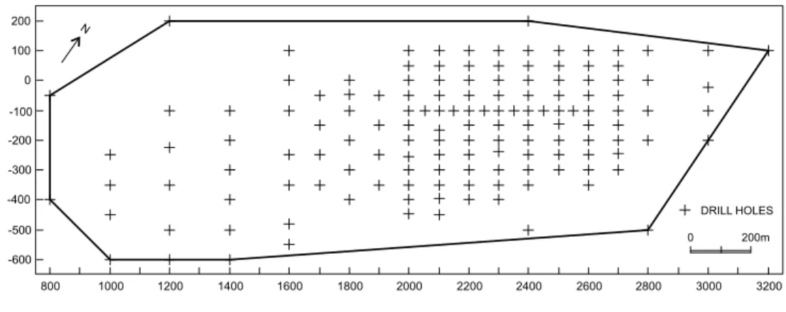
The exploration data, considered in this paper, come from 141 drill holes (Figure 7) which totalizes 16315.80 meters of continuous sampling. A total of 10504 samples analysed for copper were composited to a bench height of 10 meters resulting in 1596 composite samples and they will be the database for this study. Figure 8 shows copper grade distribution with its statistics.
So, given the boundaries of mineralization (Figure 7), the deposit is discretized into blocks of compatible dimensions with the exploration data, defined to be 100 x 100 x 10 m (width x length x height). The block model for the Chapada Copper Deposit is shown in Figure 9.
Geostatistical analysis carried out using copper exploration data resulted in the following covariogram model: Chapada Copper Deposit Crixás Uruaçu Anápolis Goiânia Rio Verde Itumbiara Brasília DF Porangatu Niquelândia BR-364 GO-060 BR-060 GO-164 GO-070 BR-153 B R -0 5 0 BR-020 BR-414 BR-1 53 BR-153 STATE OF TOCANTINS STATE OF GOIÁS STATE OF MATO GROSSO STATE OF MATO GROSSO DO SUL STATE OF MINAS GERAIS 50 km N Brazil 52º 50º 48º 46º 12º 14º 16º 18º
FIGURE 6 - Location map of the Chapada Copper Deposit. ( ) ( ) ( ) ( ) ( ) ( ) ( ) ( ) ( ) ( ) ( ) ( ) ⎥ ⎥ ⎥ ⎥ ⎥ ⎥ ⎦ ⎤ ⎢ ⎢ ⎢ ⎢ ⎢ ⎢ ⎣ ⎡ − − − = ⎥ ⎥ ⎥ ⎥ ⎥ ⎥ ⎦ ⎤ ⎢ ⎢ ⎢ ⎢ ⎢ ⎢ ⎣ ⎡ ⎥ ⎥ ⎥ ⎥ ⎥ ⎥ ⎦ ⎤ ⎢ ⎢ ⎢ ⎢ ⎢ ⎢ ⎣ ⎡ − − − − − − − − − 1 0 1 1 1 1 1 1 2 1 2 1 2 1 2 2 2 1 2 1 2 1 1 1 ' n o o o ' n ' n ' n ' n ' n ' n ' n x x x x x x w w w x x x x x x x x x x x x x x x x x x φ φ φ µ φ φ φ φ φ φ φ φ φ M M L L M M L M M L L
( )
( )
⎪ ⎩ ⎪ ⎨ ⎧ > = ≤ ⎥ ⎥ ⎦ ⎤ ⎢ ⎢ ⎣ ⎡ ⎟ ⎠ ⎞ ⎜ ⎝ ⎛ + ⎟ ⎠ ⎞ ⎜ ⎝ ⎛ − = m a if h C m a if a h a h . h C 450 0 450 2 1 2 3 1 027 0 3 (22)Geometrical anisotropy (parallel to the coordinate axes) was recognized according to the anisotropy ratios of Table 2.
Now we have the necessary elements to perform grade estimation in blocks or at points by ordinary kriging and make comparisons with radial basis functions.
4.1 Choosing a basis function
The first step for radial basis function interpolation is related to choosing an adequate kernel or basis function. This step corresponds to the variogram modeling for ordinary kriging estimation. Among several available options for basis functions we have to choose one, which could give unbiased results. Moreover, in geology we also have to consider the geological correlation between samples, i.e. there is a maximum distance within which samples present a correlation. Beyond this maximum distance samples are not correlated, when changes in composition, lithology and other physical and chemical properties usually occur and, therefore, cannot be predicted. Therefore, a maximum distance between samples and the point to be interpolated should be taken into account. For the case study, as we have a covariogram model, a maximum distance equal to 450 m (corresponding to the variogram range) will be used.
Our main concern when choosing a basis function is related to the metrics involved, because distances between samples are measured in meters (tens to hundreds of meters). So, some basis functions like cubic and splines are not convenient, because the rounding errors in the floating-point arithmetic can lead to innacurate results.
The cross validation method was adopted as a standard testing procedure to choose a basis function. This procedure consists of removing each
800 1000 1200 1400 1600 1800 2000 2200 2400 2600 2800 3000 3200 -600 -500 -400 -300 -200 -100 0 100 200 0 200m DRILL HOLES N
FIGURE 7 - Location map of drill holes from Chapada Copper Deposit and boundaries of mineralization.
TABLE 2 - Anisotropy ratios for the copper semivariograms.
direction anisotropy ratio
horizontal 2.25 vertical 4.50 0 5 10 15 0.00 0.50 1.00 1.50 2.00 COPPER Number of Data = 1596 Mean = 0.280 Standard Deviation = 0.208 Coefficient of Variation = 0.743 Maximum = 1.724 Upper Quartile = 0.372 Median = 0.231 Lower Quartile = 0.124 Minimum = 0.011 (%)
sample from the database in turn and estimating the value at that location using n’ neighboring points. So, for each point we have the actual: F(xi) and estimated: F*(xi) values which can be compared, giving us an indication of how well the basis function fits into the data. Some statistics can be computed from the difference between true and estimated values such as: correlation coefficient and RMS error. RMS error (MADYSH, 1992) was computed using:
( )
( )
[
]
∑
=−
=
N i i iF
*
x
x
F
N
RMS
1 21
which measures the dispersion of estimated values around true ones. Another way for evaluating basis function can be done by determining the condition number of a matrix of the system of equations (20). The condition number of matrix tells us how invertible the matrix is. If the condition number is infinite the matrix is singular, and ill-conditioned if it is too large (PRESS et al., 1989). A procedure available in PRESS et al. (1989) for singular value decomposition was used to compute the condition number of a matrix.
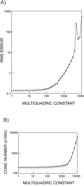
So, several simulations were carried out for the Chapada database in order to choose a multiquadric constant (c), which would give the minimum RMS error. In these simulations c values ranging from 1 to 10000 were used. Figure 10A shows RMS error as a function of the multiquadric constant c. In such figure we observe that the multiquadric constant should be chosen as small as possible. It is important to mention that the multiquadric constant
only causes round off errors and it practically does not affect the condition number of the matrix as shown in Figure 10B, with magnitudes ranging from 105 to 106. In Figure 10 both RMS error and condition number are represented as their averages coming from 1596 interpolated points.
According to obtained results from cross validation tests, the multiquadric constant must be as small as possible. Therefore, we have adopted a constant equal to 1, which best fits to the exploration data from Chapada. Actually, we will adopt hereafter in this paper the translated linear kernel: 1 2 3 4 5 6 7 8 9 10 11 12 13 14 1516 17 18 19 20 21 2223 24 25 J-AXIS 1 2 3 4 5 6 7 8 9 I-AXIS 18 17 16 15 14 13 12 11 109 8 7 6 5 43 2 1 K-AXIS 3178
FIGURE 9 - Three-dimensional model of blocks for the Chapada Copper Deposit and the block 3176.
1 10 100 1000 10000 0.1 1 10 100 1000 RMS ERROR MULTIQUADRIC CONSTANT
A)
FIGURE 10 - Influence of the multiquadric constant over estimates as measured by RMS error (A) and over condition number of matrices (B).
1 10 100 1000 10000 100 1000 10000 COND. NUMBER (x1000) MULTIQUADRIC CONSTANT
B)
( )
x
= x
+
1
φ
. Now we are interested incomparative tests between different interpolation techniques: inverse distance weighting, ordinary kriging and radial basis function with the translated linear kernel. In case of the inverse distance weighting a power of distance equal to 2 was considered. Table 3 presents the statistics for cross validation tests.
Scattergrams for the cross validation results are presented in Figure 11.
The best result is achieved with ordinary kriging, followed by radial basis functions and finally by inverse distance weighting. When using radial basis functions the metrics involved is important and it will govern the accuracy of the estimates. So, in order to improve the estimates using radial basis functions some transformations on the translated TABLE 3 - Statistics of cross validation tests for the Chapada data base.
Method Parameter Correlation RMS error
coefficient
inverse distance weighting p=2 0.748 0.140
Ordinary kriging covariance function 0.757 0.137
radial basis function translated linear kernel 0.751 0.139
TABLE 4 - Statistics of cross validation tests using radial basis functions with transformed kernels.
Transformed kernel Correlation coefficient RMS error Condition number
Square root 0.757 0.137 1.31912E03
Natural logarithm 0.761 0.136 2.44678E02
Decimal logarithm 0.761 0.136 4.79738E01
FIGURE 11 - Scattergrams for cross validation results using: A) inverse distance weighting; B) ordinary kriging and C) radial basis functions with translated linear kernel.
TR U E V A LU E ESTIMATED VALUE 0 0.50 1 1.50 0 0.50 1 1.50 0 0.50 1 1.50 0.50 1 1.50 0 0.50 1 1.50
A)
B)
C)
FIGURE 12 - Transformed kernels for radial basis functions (square root is represented as: −1+ x +1).
0 1 2 3 0 5 10 15 DISTANCE T R AN SF O R M E D K E R N EL ln(Ix I+1) IxI+1 log(IxI+1)
linear kernel were considered. These transforms are as follows: Square root:
( )
x
= x
+
1
φ
Natural logarithm:φ
( )
x
=
ln
(
x
+
1
)
Decimal logarithm:φ
( )
x
=
log
(
x
+
1
)
Transformed kernels are illustrated in Figure 12. Table 4 presents computed statistics on scattergrams as well as the average condition number for estimates using radial basis functions with transformed kernels. As we can see, transformedkernels present average condition number much lesser than the multiquadric kernel. It means that besides the inversion problem on matrix of the system of equations (20), the round off errors as seen in Figure 10A can be avoided.
Figure 13 presents scattergrams of cross validation tests using radial basis functions with transformed kernels.
Indeed transformed kernels improve estimates as shown in scattergrams of Figure 13, because the accuracy of the radial basis functions depends strongly on the metrics used. Moreover, transformed kernels effectively diminish the condition number of matrix (Table 4). So, as we can see it is nonsense to
TRUE V ALUE ESTIMATED VALUE 0 0.50 1 1.50 0 0.50 1 1.50 0 0.50 1 1.50 0.50 1 1.50 0 0.50 1 1.50
A)
B)
C)
FIGURE 13 - Scattergrams for cross validation results using transformed kernels: A) square root; B) natural logarithm, C) decimal logarithm.
A) B)
TRUE
V
ALUE
INVERSE OF WEIGHTED DISTANCE
0 0.50 1 1.50 0 0.50 1 1.50 TRUE V ALUE RBF (LINEAR) 0 0.50 1 1.50 0 0.50 1 1.50
FIGURE 14 - Comparison of ordinary kriging against inverse distance weighting (A) and radial basis functions using linear kernel with no transformation (B).
consider other kernels like cubic and splines, because they rise rapidly with x. Therefore, all the transformations were done over the translated linear kernel. See that the transformed kernels limit the influence of far samples as well as the variogram does.
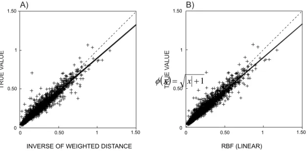
Considering that ordinary kriging gives the best results, let us compare it with inverse distance weighting and radial basis functions with no transformation (Figure 14).
Figure 14 shows that both methods provide biased estimates in relation to the ordinary kriging. Therefore, they cannot be used for reliable ore reserve estimation. Now let us verify if the transformed kernels provide better results than kernels with no transformation. Figure 15 presents scattergrams of ordinary kriging estimates against radial basis functions using transformed kernels.
As we can see square root is not an effective transformation for the database of the study case, because of the metrics involved (hundreds of meters). On the other hand, natural and decimal logarithms are the most effective giving the best results. Both give almost unbiased and basically the same results, which proves that kernel transformation provides good estimates comparable to the ordinary kriging results. The dispersion around the bisector may be due to the differences between spherical covariance (kernel for ordinary kriging) and transformed kernel (natural or decimal logarithm). Moreover, there is also the correction for geometrical anisotropy done by ordinary kriging while radial basis functions do not. Radial basis functions with appropriate kernels give reliable results being comparable to the ordinary kriging ones. Hence, radial basis function is another
method available for ore reserve estimation.
5 CONCLUDING REMARKS
Radial basis function estimator with a constant precision term has a dual form absolutely equivalent to the ordinary kriging estimator. Hence, radial basis function arises as an alternative method to ordinary kriging, especially in cases where experimental variograms cannot be computed from data points. This method is much better than the inverse distance weighting, which has been used as an alternative to the ordinary kriging. Radial basis function is superior to the inverse distance weighting, because it can recognize clustered points giving adequate weights according to their spatial configuration, such as done by ordinary kriging. Accurate results from radial basis function estimates depend strongly on metrics involved and also on kernels. The linear kernel with a logarithmic transformation gives the best result for exploration data from the Chapada Copper Deposit, as confirmed by average condition number of matrices.
6 REFERENCES
ARMSTRONG, M. 1994. Is research in mining as dead as a dodo? In: R. Dimitrakopoulos (ed.) Geostatistics for the next century. Dordrecht, Kluwer Academic Publishers, p. 303-312. BARNHILL, R.E. 1993. A survey on the
representation and design of surfaces. IEEE Computer Graphics & Applications, 3(3): 9-16.
ORDINAR Y KRIGING 0 0.50 1 1.50 1.50 0.50 1 1.50 RBF (SQUARE ROOT) 0 0.50 1 0 0.50 1 1.50 0 0.50 1 1.50
A)
B)
C)
FIGURE 15 - Comparison of ordinary kriging estimates against radial basis functions using transformations by: square root (A), natural logarithm (B) and decimal logarithm (C).
BEATSON, R.K. & NEWSAM, G.N. 1992. Fast evaluation of radial basis functions: I. Comput. Math. Applic., 24(12): 7-19.
CARLSON, R.E. & FOLEY, T.A. 1992. Interpolation of track data with radial basis methods. omput. Math. Applic., 24(12): 27-34.
FOLEY, T.A. 1992. The map and blend scattered data interpolation on a sphere. Comput. Math. Applic., 24(12): 49-60.
GIROSI, F. 1992. Some extensions of radial basis functions and their applications in artificial intelligence. Comput. Math. Applic., 24(12): 61-80.
HARDY, R.L. 1971. Multiquadric equations of topography and other irregular surfaces. J. Geophys. Res., 76(8): 1905-1915.
HARDY, R.L. 1977. Least square prediction. Phot. Eng. & Rem. Sensing, 43(4): 475-492.
ISAAKS, E.H. & SRIVASTAVA, R.M. 1989. An introduction to applied geostatistics. New York, Oxford University Press. 561p.
JOURNEL, A.G. & HUIJBREGTS, C.J. 1978. Mining geostatistics. London, Academic Press. 600p. KANSA, E.J. 1990. Multiquadrics – a scattered d a t a a p p r o x i m a t i o n s c h e m e w i t h a p p l i c a t i o n s t o c o m p u t a t i o n a l f l u i d -dynamics – I. Comput. Math. Applic., 19(8/ 9): 127-145.
MADYCH, W.R. 1992. Miscellaneous error bounds for multiquadric and related interpolators. Comput. Math. Applic., 24(12): 121-138.
MICCHELLI, C.A. 1986. Interpolation of scattered data: distance matrices and conditionally positive definite functions. Constr. Approx., 2:11-22. MYERS, D.E. 1992. Kriging, cokriging, radial basis
functions and the role of positive definiteness. Comput. Math. Applic., 24(12): 139-148. OLEA, R. 1991. Geostatistical glossary and
multilingual dictionary. New York, Oxford University Press. 175p.
PHILIP, G.M. & WATSON, D.F. 1987. How ore deposits can be overestimated through computational methods. In: AIMM, RESOURCES AND RESERVES SYMPOSIUM, Melbourne, Proceedings: 49-58.
PRESS, W.H.; FLANNERY, B.P.; TEUKOLSKY, S.A.; VETTERLING, W.T. 1989. Numerical recipes in Pascal. Cambridge, Cambridge University Press. 759p.
SIRAYANONE, S. 1988. Comparative studies of kriging, multiquadric-biharmonic and other methods of solving mineral resources problems. Iowa State University, Ames, Ph. D. Dissertation, 355p.
WACKERNAGEL, H. 1995. Multivariate geostatistics: an introduction with applications. Berlin, Springer-Verlag, 256p.
YAMAMOTO, J.K. 1996. A new method of block calculation using the inverse of weighted distance. Engineering & Min. J., 197(9):69-72. YAMAMOTO, J.K. 2000. An alternative measure of the reliability of ordinary kriging estimates. Math. Geology, 32(4): 489-509.
Author’s address:
Jorge Kazuo Yamamoto – Instituto de Geociências, Universidade de São Paulo, Caixa Postal 11.348, CEP 05422-970, São Paulo, SP, Brasil. E-mail: [email protected]