www.ann-geophys.net/26/3831/2008/ © European Geosciences Union 2008
Annales
Geophysicae
Comparison of methods to determine auroral ionospheric
conductances using ground-based optical and riometer data
A. Senior, M. J. Kosch, and F. Honary
Dept. of Communication Systems, Lancaster University, Lancaster, LA1 4WA, UK
Received: 20 June 2008 – Revised: 2 September 2008 – Accepted: 21 October 2008 – Published: 2 December 2008
Abstract.Ground-based images of auroral optical emissions and cosmic radio noise absorption provide information on particle precipitation which enhances ionospheric conduc-tances. Knowledge of this conductance field is important to understand the current systems associated with auroral fea-tures. Three methods of using ground-based optical and ri-ometer data to estimate ionospheric conductances in the au-rora are compared to conductances derived from incoherent scatter radar measurements. It is shown that a method using the 557.7 nm emission intensity alone gives the best results for the Pedersen conductance whilst a method using both this intensity and cosmic noise absorption is best for the Hall con-ductance. A method using cosmic noise absorption alone gives reasonable performance for the Hall conductance and the Hall/Pedersen conductance ratio, but performs poorly for the Pedersen conductance. It also appears to underestimate the Hall conductance significantly during times when softer precipitation is present, for example in discrete auroral arcs. There is some indication that the methods do not degrade no-ticeably for angles up to∼20◦off magnetic zenith.
Keywords. Ionosphere (Auroral ionosphere; Electric fields and currents; Ionosphere-magnetosphere interactions)
1 Introduction
In studies of the aurora, it is important to be able to under-stand the spatial structure of the electrical current systems which couple the magnetosphere and ionosphere. The cur-rents can be measured in situ by spacecraft, or inferred from ground-based magnetometer measurements. However, the former cannot “image” the two-dimensional distribution of currents (without many spacecraft) and the latter is insensi-tive to the curl-free part of the current system (Amm, 1997). Correspondence to:A. Senior
The currents can be indirectly determined from Ohm’s Law if the electric field and conductivity distributions are known. The former can be obtained from ground-based coherent scatter radars (Greenwald et al., 1978, 1995) on global and meso-scales (∼10–100 km). The latter can be obtained on global scales by inverting spacecraft measurements of auro-ral emissions (e.g. Aksnes et al., 2006), but these lack the resolution for meso-scale studies around individual auroral arcs. In those cases, ground-based measurements of opti-cal emissions and cosmic radio noise absorption (CNA) give information on the precipitating electrons which create the ionisation leading to conductivity and these can be used to determine the meso-scale conductivity distribution.
In this study, three different methods of determining the ionospheric height-integrated conductivities (conductances) from optical and CNA measurements are compared. As a ref-erence, the conductances derived from EISCAT incoherent scatter radar measurements are used. All three methods were originally calibrated by such measurements, but the data sets used here were not used in those calibrations and in that sense provide an independent test. The main aim of this study is to investigate under what circumstances each method performs well or poorly and consequently what might be required to form a better approach.
2 The methods tested
The three methods under test in this study are summarised as follows.
2.1 Statistical relationships using CNA alone (S07) Senior et al. (2007) presented a set of statistical relationships between cosmic noise absorption and the Hall and Pedersen conductances and their ratio for five different sectors of MLT. The relationships were derived by comparing conductances calculated from EISCAT measurements with CNA measure-ments from the nearby imaging riometer at Kilpisj¨arvi in Fin-land. Senior et al. (2007) fitted power-law functions to the data arguing that these seemed most suited to the data in the absence of any simple physical argument to support another form of function. The relationships had the most explain-ing power for the Hall conductance. Hereinafter, this method will be referred to as “S07”.
2.2 Statistical relationship using 557.7 nm intensity alone (K98)
On the basis that the 557.7 nm column emission rate (inten-sity) is proportional to the flux of precipitating electrons and that the Pedersen conductance is proportional to the square-root of this flux, Kosch et al. (1998b) fitted the conductance (6P in S) to the square-root of the intensity (I in rayleighs):
6P =0.34+0.18
√
I (1)
The study considered both pre- and post-magnetic midnight time sectors and found no significant difference in the rela-tionship between these sectors. The data sets used spanned ∼19.5–05.5 MLT with most of the data in the 21.5–03.5 MLT interval. Interestingly, Senior et al. (2007) found that the conductance-CNA relationships were more-or-less constant during the 19:00–04:00 MLT interval.
2.3 “Energy map” method (K01)
Kosch et al. (2001) combined both CNA and the 557.7 nm column intensity to estimate the characteristic energy of elec-tron precipitation. Their approach was to use measurements to calibrate a simple physical model of the CNA and optical intensity in terms of the characteristic energy for assumed Maxwellian or exponential precipitating electron spectra. The objective was to produce high spatial-resolution maps of characteristic energy from imaging riometer and all-sky camera images, hence the description “energy map”. As the method gives only the energy and not the flux, only the Hall/Pedersen conductance ratio can be directly determined by this approach. Here, the method is extended to determine the flux for the case of a Maxwellian spectrum.
Kosch et al. (2001) made the assumption that the 38.2 MHz CNA (Ain dB) is proportional to the square-root of the flux of precipitating electrons with energies exceeding
25 keV (825): A=k825. The differential number fluxφ(in cm−2s−1keV−1) for a Maxwellian spectrum is
φ= 8
E02Eexp(−E/E0) (2)
where E is the energy in keV, 8 is the integral flux in cm−2s−1andE
0is the characteristic energy in keV. The
dif-ferential flux peaks whenE=E0. The flux of electrons with energies exceeding 25 keV is then
825=
Z ∞
25 8
E02Eexp(−E/E0)dE
=8
1+ 25
E0
exp
−E25
0
(3) and hence
A=k
s
8
1+ 25
E0
exp
−25
E0
(4) wherekis a constant to be determined.
The dataset used by Kosch et al. (2001) gives values of 8andE0from the inversion of the EISCAT electron
den-sity profiles and the corresponding CNA data measured by the IRIS riometer (see Sect. 3.1). The fluxes used by Kosch et al. (2001) are differential in pitch angle; to convert these to fluxes integral in pitch angle over the downward hemi-sphere as used here, the Kosch et al. (2001) fluxes are mul-tiplied by 2π. Figure 1 presents the data and the least-squares fit of Eq. (4). Note that, in keeping with Kosch et al. (2001), points where the CNA was less than 0.07 dB have been excluded. The relationship is reasonably linear with a Pearson correlation coefficient of 0.8. The fit gives k=2.4×10⁻⁴dB cm s1/2. This result appears to be
reason-ably consistent with the empirical relations quoted in Ta-ble 1 of Hargreaves (1969) when the difference in riometer frequency (30 MHz versus 38.2 MHz) and minimum energy (40 keV versus 25 keV) is accounted for.
Having established this relationship and given measure-ments of the CNA and 557.7 nm intensity the integral flux8 can be determined by first findingE0using Eq. (18) of Kosch
et al. (2001): loge√A
I =1.0−
8.8
E0
(5) where I is the 557.7 nm intensity in kR and then solving Eq. (4) for8. Finally, the Hall (6H) and Pedersen (6P) conductances can be estimated from8andE0by applying
the formulae of Robinson et al. (1987):
6P =
40E¯ 16+ ¯E28
1/2
E (6)
6H
6P =
0.45(E)¯ 0.85 (7)
0 500 1000 1500 2000 2500 3000 3500 4000 0
0.2 0.4 0.6 0.8 1 1.2 1.4
Φ250.5 (cm−1 s−0.5)
A (dB)
13 February 1996 9 November 1998
Fig. 1.Scatter plot of absorptionAversus the square-root of the flux of electrons with energies exceeding 25 keV (825) for the Kosch et al. (2001) data. The line is the least-squares fit of Eq. (4) to all points.
are given by E¯=2E0 and8E≈1.6×10−9×2E08,
respec-tively, taking account of the units of 8. Hereinafter, this method will be referred to as “K01”. The original Kosch et al. (2001) method has been evaluated by Ashrafi et al. (2005).
3 Observations
3.1 Instrumentation
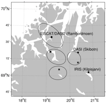
The locations of all the instruments used in this study are shown in Fig. 2. The EISCAT UHF incoherent scatter radar is located at Ramfjordmoen, near Tromsø, Norway (69.58◦N, 19.22◦E; Rishbeth and van Eyken, 1993). In this
study we use two intervals of data, one from 8/9 March 1999 (Case 1) and the other from 23 November 2006 (Case 2). These intervals were selected due to the conjunction of avail-able data from the radar and the all-sky imager and riometer used and also because they contain significant auroral activ-ity over several hours. In Case 1, the radar was operating in the Common Programme 2 mode, where the antenna is scanned between four different look directions with a dwell time of∼90 s on each position, making a 6-min cycle. The look directions are vertical, magnetic field-aligned (azimuth 183.2◦, elevation 77.2◦), (166.5◦, 62.9◦) and (133.3◦, 60.4◦).
The data have been integrated over the periods when the an-tenna was stationary in each direction. In Case 2, the radar was directed field-aligned (185.1◦, 77.5◦) and the data were
integrated in 60 s blocks.
18oE 19oE 20oE 21oE
45’
69oN
15’ 30’ 45’
70oN
IRIS (Kilpisjarvi) EISCAT/DASI2 (Ramfjordmoen)
DASI (Skibotn)
Fig. 2.The locations of the instruments used in this study, marked by the squares. The rings indicate the−3 dB contours of four IRIS beams at 90 km altitude. The crosses mark the locations of the EIS-CAT radar beam at 110 km for all the scan positions used (note that the vertical position overlaps the instrument location).
The CNA measurements come from the IRIS imaging ri-ometer at Kilpisj¨arvi, Finland (69.05◦N, 20.79◦E; Browne
et al., 1995). The riometer produces a 7×7 array of beams of widths (full width at −3 dB) between 11◦ and 14◦,
corresponding to 18 km horizontally at 90 km altitude at the zenith. The field-of-view at 90 km is approximately 200×200 km. The locations of the beams relevant for this study are shown in Fig. 2. The fundamental temporal resolu-tion is 1 s.
In Case 1, 557.7 nm intensities are taken from the Dig-ital All-Sky Imager (DASI) at Skibotn, Norway (69.35◦N,
20.36◦E; Kosch et al., 1998a). DASI records a 557.7 nm
3.2 Data processing
Since electron precipitation is geomagnetic field-aligned, it makes sense to compare measurements along the same mag-netic field line as closely as possible. Due to the different instrument locations and look-directions, this was achieved approximately as follows.
The reference field-line was defined as the one on which the EISCAT radar beam intersected an altitude of 110 km. This height was chosen as intermediate between the Ped-ersen and Hall conductance layers. The location of this intersection was then found in AACGM co-ordinates (for-merly PACE; Baker and Wing, 1989). In this system, all points on the same field line have the same latitude and lon-gitude. The 557.7 nm and CNA images were transformed into AACGM co-ordinates assuming a typical altitude for the 557.7 nm emission of 100 km (Kosch et al., 1998b) and a typical altitude for the absorbing layer of 90 km (Hargreaves, 1969). The images were then linearly interpolated to the co-ordinates of the field-line previously defined. In fact, since the geomagnetic field is inclined only about 12◦to the
ver-tical, the horizontal alignment error in using geographic co-ordinates instead of AACGM would only be 4 km between the nominal conductance and CNA altitudes, smaller than the resolution of IRIS and DASI.
Matching of the data in time was achieved by integrating the camera and riometer measurements over each radar gration period. In the case of DASI2, where the image inte-gration time is much less than the interval between images, this means that the integration does not take place over the complete radar integration period.
In Case 1, the 557.7 nm intensities were scaled up by a factor of 2.8. Without this scaling, the K98 method gave Pedersen conductance estimates that agreed closely in the shape of the time series, but were too small in magnitude compared to the radar-derived values. Additionally, the K01 method underestimated the characteristic energy and hence the Hall/Pedersen conductance ratio (the individual conduc-tance estimates were also incorrect) compared to the radar. This single scaling factor, applied to the entire Case 1 data set, corrected this problem. The need for this scaling is not fully understood, but possibly there was a calibration prob-lem with the DASI instrument at this time. A comparison of stellar intensities in an adjacent white-light imager be-tween Case 1 and another night with clear sky showed no significant difference, suggesting that thin cloud was not to blame. This discrepancy does not seem to have been found by Ashrafi et al. (2005) who looked at data before and af-ter the date in question which suggests it was a temporary problem. No such scaling was required in Case 2 which uses the newer DASI2 instrument for which the calibration had recently been determined using both stellar intensities and radioluminescent sources with good agreement.
The EISCAT plasma parameters were used to calculate the Hall and Pedersen conductivities and these were
height-integrated over the altitude range 92–200 km to give the cor-responding conductances in the manner described by Senior et al. (2007). The 557.7 nm intensities and CNA were used to estimate the conductances according to the three methods under test.
There are a number of possible sources of error in the data. Random error in the radar measurements contributes to ran-dom error in the conductances. The contribution to this from the error in the electron density is easy to assess. In Case 1, for the Hall conductance, 57% (96%) of points have errors less than 1% (5%); for the Pedersen conductance the corre-sponding proportions are 84% and 100% and for the conduc-tance ratio, 38% and 96%. In Case 2, the proportions are 0% and 97% for the Hall conductance; 0% and 99% for the Pedersen conductance and 0% and 95% for the ratio. The er-rors are sufficiently small that one-standard-error error-bars on the plots are almost invisible, except for a few cases in the conductance ratio. Here, only the error bars for the ratio are presented. These error estimates are all underestimates because the contribution to the error from the uncertainty in the temperature measurements, which is more complicated to assess, is not included.
Besides random errors, there may also be systematic er-rors. Firstly, as the radar beam was not always directed field-aligned and the 557.7 nm emission and CNA do not come from thin layers at fixed heights, there are ambiguities in the spatial correspondence of the measurements. Secondly, tem-poral ambiguities can arise because the quantities measured by the different instruments have different response time con-stants to changes in the precipitating particle flux. Thirdly, there can be systematic errors in the radar data analysis due to assumptions such as the ion composition being incorrect. The latter can also affect the calculation of the conductances. Furthermore, as the radar coverage stops at about 92 km al-titude, the Hall conductance may be underestimated as the Hall conductance region can extend below this altitude.
3.3 Case 1: 8/9 March 1999
Figure 3 shows the observations from 8/9 March 1999 (18:30–03:00). All times herein are in UT unless other-wise stated. The geomagneticKpindicies during the period were 2+ (18:00 UT), 4+ (21:00 UT), 4− (00:00 UT) and 4
21:17:40 22:04:00 01:14:30 01:53:40
Altitude (km)
20 22 00 02
100 150 200 250 300
log
10
N
e
(m
−3
)
10 11 12
Σ H
(S)
A B
C
D
20 22 00 02
0 20 40 60 80 100
Σ P
(S)
20 22 00 02
0 10 20 30 40
Σ H
/
Σ P
UT
20 22 00 02
0 2 4 6 EISCAT
S07 K01 K98
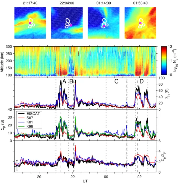
Fig. 3.Data from 8/9 March 1999 (Case 1). The methods are identified by the line colours which are labelled in the fourth row. The dotted vertical lines mark intervals of interest which are labelled in the third row. The dashed vertical lines mark the times of the images in the top row. Top row: 557.7 nm images. The intensity scale covers the range of the data in each image and the intensities have been compressed by taking the square-root to reveal weaker features. The white rings indicate the−3 dB contours of a subset of IRIS beams. The pink crosses indicate the EISCAT UHF beam direction. The images are presented in AACGM co-ordinates (latitudes 64.83–67.83, longitudes 100.62–106.62) with north to the top and east to the right. Second row: electron densities from the EISCAT UHF radar. Third row: Hall conductances. Fourth row: Pedersen conductances. Bottom row: Hall/Pedersen conductance ratio. The one standard error bound is shown by error bars where the error exceeds 0.25.
gaps in the time series for the K01 method are discussed in Sect. 4.3.
The image at 21:17:40 was taken close to the peak of the conductance enhancement in interval A. It shows a roughly east-west aligned arc. The structures in the arc appear to have scales similar to the size of the IRIS beams. The elec-tron density profiles are enhanced over the height range 90– 200 km (sometimes higher) during interval A. Both the S07 and K01 methods underestimate the Hall conductance
dur-ing this interval, the former especially so. The S07 method also underestimates the Pedersen conductance significantly, though it reproduces the Hall/Pedersen ratio rather well.
20:23:20 20:48:05 21:37:35 22:48:05
Altitude (km)
20:30 21:00 21:30 22:00 22:30
100 150 200 250 300
log
10
N
e
(m
−3
)
10 11 12
Σ H
(S)
A
B
C
20:30 21:00 21:30 22:00 22:30
0 20 40 60 80 100
Σ P
(S)
20:30 21:00 21:30 22:00 22:30
0 20 40 60
Σ H
/
Σ P
UT
20:30 21:00 21:30 22:00 22:30
0 1 2 3 EISCAT S07 K01 K98
Fig. 4.Data from 23 November 2006 (Case 2). The format is as for Fig. 3.
the conductances. The S07 estimate of the Hall/Pedersen ra-tio is again rather good.
The image at 01:14:30 was taken near the end of inter-val C when the overestimate of the Pedersen conductance by the K01 method was greatest. The 557.7 nm emission shows some discrete structure of a similar scale-size to the IRIS beams. The electron density profiles are enhanced mainly in the 100–150 km interval with occasional enhancements to higher altitudes. Here, the S07 method estimates the conduc-tances and their ratio quite well, but the K01 method overes-timates the Hall and particularly the Pedersen conductances. Finally the image at 01:53:40 was taken near the peak of the first conductance enhancement in interval D. Images cov-ering the full camera field-of-view (not shown) show that the bright emission is associated with an “omega band” structure (Opgenoorth et al., 1983) of which successive waves cause
the two enhancements in interval D. The image shows some structuring of the 557.7 nm emission in the bright region. The electron density profiles show considerable enhance-ment over altitudes from 90–200 km or higher. In interval D, all three methods underestimate the conductances, especially the S07 method, which also overestimates the Hall/Pedersen conductance ratio.
3.4 Case 2: 23 November 2006
In interval A, there is a series of diminishing conduc-tance enhancements. The K01 method estimates these well, whereas the S07 method greatly underestimates the first one, progressively getting better during the interval. The image at 20:23:20 is close to the peak of the first enhancement. It shows a mixture of discrete arc structures and more dif-fuse emission. The image at 20:48:05 is close to the end of the interval where the conductance is diminishing. It shows that the IRIS beams view a region of diffuse emission with a steady gradient across the beams.
The image at 21:37:35 is close to the peak of the conduc-tance enhancement in interval B. It shows that an east-west arc lies close to magnetic zenith, covering one beam of IRIS but only grazing the other. The arc is particularly intense in a narrow (∼6 km) strip on its poleward edge. This strip is much narrower than the IRIS beam dimensions. In this inter-val, the S07 method completely fails to estimate the large en-hancement in conductivity associated with this arc. The K01 method performs well for the Hall conductance but overes-timates the Pedersen conductance by about a factor of two. Neither the S07 nor the K01 methods correctly estimate the enhancement in the conductance ratio.
The image at 22:48:05 occurs near the start of interval C. Similarly to the end of interval A, the IRIS beams view an area of diffuse emission. The electron density profile at this time is similar in shape to that at the end of interval A. Here, the K01 method performs well for the conductances and is reasonable for their ratio. The S07 method slightly underes-timates the conductances and overesunderes-timates their ratio.
As in Case 1, the K98 method performs very well through-out the whole interval. Recall that in Case 2 no scaling was applied to the 557.7 nm intensities.
4 Discussion
Firstly, explanations for the discrepancies between the results of methods under test and the EISCAT-derived conductances are considered, followed by a statistical summary of the per-formance of the methods.
4.1 Shape of the precipitating electron spectrum
A common feature in both cases 1 (intervals A and D) and 2 (interval A) is a tendency for the S07 method to underesti-mate the conductances and to overestiunderesti-mate their ratio during periods when soft precipitation is present, as indicated by en-hanced electron densities at higher altitudes (above 150 km). Enhanced Pedersen and Hall conductances and CNA corre-spond to enhanced precipitating electron fluxes in the ap-proximate energy bands 2–10, 5–50 and>20 keV, respec-tively. There is thus considerable overlap between the bands enhancing the Hall conductance and CNA, but if there is preferential enhancement to the soft end of the spectrum, the Hall conductance may be enhanced without further
enhance-102 103 104
105
106
107
108
109
1010
1011
Energy (eV)
Flux (m
−2
s
−1 eV
−1
)
1999−03−08 18:53:40 1999−03−08 22:59:15 2006−11−23 20:23:20 2006−11−23 20:30:30 2006−11−23 22:43:40
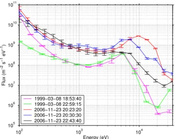
Fig. 5.Precipitating electron energy spectra derived from the EIS-CAT electron density profiles at the times shown. Error bars on each curve indicate the one standard error bound.
ment of CNA. The situation for the Pedersen conductance is even clearer as there is no significant overlap in energy band with CNA. Therefore, enhanced soft precipitation leads to an underestimate of conductances by the S07 method because the CNA contains no information on the soft part of the spec-trum. The Hall/Pedersen conductance ratio is overestimated for a similar reason.
compared to the CNA. The middle case (20:30:30) is inter-mediate both in the discrepancy between the estimates and in the shape of the spectrum. There is a clear local flux maxi-mum around 7 keV but the high-energy tail looks rather sim-ilar to that of the final case but with a higher flux. Note that as the UHF radar measurements stop at∼92 km altitude, the full extent of the height interval and hence energy range rel-evant to CNA is not covered by the data.
As the S07 method is a statistical model, one would expect to find times where overestimation occurs too. Examples of this are around 18:53 and 22:59 in Case 1. At these times, both the S07 and K01 methods overestimate the Hall con-ductance and Hall/Pedersen ratio but are somewhat closer for the Pedersen conductance. Electron spectra for these times are shown in Fig. 5 and are very similar. Overall, the fluxes are lower than in the examples from Case 2, but the notable feature is the steeper fall off in flux above the local peak at ∼5 keV. This would tend to result in less enhancement of the Hall conductance than would be the case for the spectrum shapes of the Case 2 examples.
4.2 Limited spatial resolution
In interval B in Case 2 (Fig. 4), an arc with an intense nar-row edge passed through the radar beam revealing a strong enhancement of the conductances. The 557.7 nm emission was strongly enhanced and the K98 method reproduced the Pedersen conductance rather well. However, the S07 method failed to reproduce the enhancement and the K01 method greatly overestimated the Pedersen conductance. The com-mon factor between S07 and K01 is the CNA. It is clear from the 557.7 nm images that the arc has a thickness which is small compared to the IRIS beams and the poleward beam is almost completely in a region of no emission. If the CNA has a similar morphology, it is not surprising that IRIS shows little response in this case, even though the CNA could be lo-cally strong in the arc. The spatial scale of the CNA measure-ment will almost integrate away the localised enhancemeasure-ment. This underestimate of CNA is consistent with the underesti-mate by the S07 method.
The observed 557.7 nm intensity at 21:37:35 was 39 kR and the CNA was 0.09 dB. The radar-derived Hall conduc-tance was 82 S and the Pedersen conducconduc-tance 30 S. The cor-responding K01 estimates are 75 and 59 S, respectively. It can be shown that if the CNA had been 2 dB, the K01 method would estimate the conductances as6H=81 S and 6P=30 S, so that the Hall conductance estimate is only slightly reduced whereas the Pedersen conductance is greatly reduced and matches the radar-derived value. Hence an un-derestimate of CNA due to having too-large a measurement scale could account for the failure of the K01 method in this case.
4.3 Other issues
In interval B of Case 1, all three methods overestimate the Hall and Pedersen conductances, though the S07 method es-timates their ratio quite well. Pi2 pulsations observed by the SAMNET magnetometer array (Yeoman et al., 1990) indi-cate a substorm onset just prior to 21:45, the start of inter-val B. In the DASI images (not shown except for 22:04 in Fig. 3), the 557.7 nm emission is strongest to the equator-ward edge of the field-of-view. Over interval B, the more intense 557.7 nm emission progresses poleward, but does not reach the EISCAT field-of-view until after interval B. DASI has a rather limited dynamic range (8 bits) and the intensifier gain is adjusted in realtime to compensate for this. A con-sequence is that when bright emission is present, the gain is reduced, effectively raising the noise level. It seems likely that the overestimate by K98 towards the end of interval B is a result of this effect. Regarding the IRIS CNA mea-surements, the CNA at the end of the interval was very low (∼0.1 dB) which is comparable to the error in the quiet-day cosmic noise power estimate (Senior et al., 2007).
In interval C of Case 1, the K01 method overestimates the Hall and Pedersen conductances yet estimates their ra-tio well. The origin of this behaviour can be traced to low values of CNA which fluctuate around zero; although it is unphysical, CNA can be negative as a result of an inaccurate estimate of the quiet-day noise power. An analysis of the K01 method shows that as the CNA approaches zero, so does the estimate of the characteristic energy. At the same time, the estimate of the integral number flux tends to infinity. If the CNA is zero or negative, the results become undefined. It is the delicate balance of this behaviour as the CNA tends to zero which leads to the large fluctuations, particularly in the Pedersen conductance estimate in interval C. However, since the conductance ratio depends only on the characteristic en-ergy estimate which is well-behaved even for zero CNA, the ratio estimate is also well-behaved. The gaps in the line for the K01 method correspond to those points where the CNA is zero or negative.
4.4 Statistical performance of the methods
In Case 1, the different radar look directions allow the variation in the performance of the methods with look di-rection to be explored. A comparison of the correlation coef-ficients for the results of the three methods with the EISCAT-derived conductances for each of the four radar look direc-tions showed that at the 95% confidence level, there was no significant difference between radar look directions. For IRIS, the four directions correspond to approximate angles of 25◦–52◦off magnetic zenith; for DASI the range is 2◦–34◦
and for the radar itself, the range is 0◦–23◦. It is not
possi-ble to conclude that the performance of the methods under test is relatively unaffected by angle off zenith, at least up to the limits observed, because field-aligned reference measure-ments of the conductances are not available at each location, but at least the methods become no worse than the case of a non field-aligned radar measurement. Comparing the cor-relation coefficients with the results of Case 2 (Table 1) also suggested that the results are no worse (in fact sometimes better) than for the case where both the radar and imager have field-aligned look directions.
4.5 Improvements to the methods
The S07 method performs relatively poorly compared to the K01 and K98 methods, but this is hardly surprising when one quantity (CNA) is used to describe a system with more than one degree of freedom (the precipitating electron spec-trum). Adding a second measurement as in the K01 method brings a considerable improvement. Surprisingly, the K98 method, also based on a single quantity, estimates another single quantity, the Pedersen conductance, remarkably well. The joint performance of the K01 and K98 methods suggests that there is little room for improvement to the basic method when instrumental effects such as spatial resolution and esti-mation of the riometer quiet-day level are taken away.
Temporal resolution was not investigated in this study, but modern optical imagers and riometers have good temporal resolution, comparable to or finer than the recombination time of the plasma at the altitudes of the conductance lay-ers. Therefore the data should allow short timescale changes in conductance to be monitored, although the methods might require some adaptation to account for non-equilibrium ef-fects.
5 Conclusions
The cases studied here allow the following conclusions to be drawn about the three methods tested:
1. The S07 method underestimates conductances when soft precipitation is present, for example inside auroral arcs. Overestimation is seen in some circumstances in diffuse aurora, depending on the detail of the precipitat-ing electron spectrum.
Table 1.Pearson correlation coefficients between the conductance parameter estimates from EISCAT and from the three methods un-der test. The upper number in each case is for Case 1, the lower number is for Case 2.
Parameter K98 K01 S07
6H 0.98 0.87
0.97 0.63 6P 0.96 0.90 0.71 0.97 0.88 0.55
6H/6P 0.70 0.78
0.56 0.73
2. Despite the above, the S07 method provided the best estimates of the Hall/Pedersen conductance ratio. 3. The K01 method provided the best estimates of the Hall
conductance.
4. The K98 method provided the best estimates of the Ped-ersen conductance.
5. Insufficient spatial (and presumably temporal) resolu-tion in the measurements can lead to serious errors in the conductance estimates.
6. There is no evidence for a deterioration in the perfor-mance of the methods at least up to magnetic zenith an-gles of∼20◦. This is a conservative estimate based on
the maximum magnetic zenith angle of the radar mea-surement.
It is worth noting that the results show that when the esti-mation of “bulk” parameters such as the conductances are required, as opposed to height-resolved conductivities or the spectrum of precipitating particles, good results can be ob-tained using only one or two ground-based measurements. Acknowledgements. This work was supported by grant PP/C000218/1 from the UK Particle Physics and Astronomy Research Council (now the Science and Technology Facilities Council (STFC)). IRIS and SAMNET are funded by STFC. EISCAT is an international association supported by research organisations in China (CRIRP), Finland (SA), France (CNRS, till end 2006), Germany (DFG), Japan (NIPR and STEL), Norway (NFR), Sweden (VR), and the United Kingdom (STFC). We are very grateful to B. Gustavsson (U. Tromsø) and U. Br¨andstr¨om (IRF, Kiruna) for their assistance in calibrating the DASI2 instru-ment. We thank the reviewers for their constructive criticism of the manuscript.
Topical Editor M. Pinnock thanks R. Makarevich and A. Brekke for their help in evaluating this paper.
References
profiles of the ionospheric electron density derived using space-based remote sensing of UV and X ray emissions and EISCAT radar data: A ground truth experiment, J. Geophys. Res., 111, A02301, doi:10.1029/2005JA011331, 2006.
Amm, O.: Ionospheric elementary current systems in spherical co-ordinates and their application, J. Geomag. Geoelectr., 49, 947– 955, 1997.
Ashrafi, M., Kosch, M. J., and Honary, F.: Comparison of the char-acteristic energy of precipitating electrons derived from ground-based and DMSP satellite data, Ann. Geophys., 23, 135–145, 2005,
http://www.ann-geophys.net/23/135/2005/.
Baker, K. B. and Wing, S.: A new magnetic coordinate system for conjugate studies at high-latitudes, J. Geophys. Res., 94, 9139– 9143, 1989.
Browne, S., Hargreaves, J. K., and Honary, B.: An Imaging Riome-ter for Ionospheric Studies, Electron. Commun. Eng., 7, 209– 217, 1995.
Greenwald, R. A., Weiss, W., Nielsen, E., and Thomson, N. R.: STARE: A new radar auroral backscatter experiment in northern Scandinavia, Radio Sci., 13, 1021–1039, 1978.
Greenwald, R. A., Baker, K. B., Dudeney, J. R., Pinnock, M., Jones, T. B., Thomas, E. C., Villain, J. P., Cerisier, J. C., Senior, C., Hanuise, C., Hunsucker, R. D., Sofko, G., Koehler, J., Nielsen, E., Pellinen, R., Walker, A. D. M., Sato, N., and Yamagishi, H.: DARN/SUPERDARN: A global view of the dynamics of high-latitude convection, Space Sci. Rev., 71, 761–796, 1995. Gustavsson, B.: Tomographic inversion for ALIS noise and
resolu-tion, J. Geophys. Res., 103, 26 621–26 632, 1998.
Hargreaves, J. K.: Auroral absorption of HF radio waves in the ionosphere: a review of results from the first decade of riome-try, Proc. IEEE, 57, 1348–1373, 1969.
Janhunen, P.: Reconstruction of electron precipitation characteris-tics from a set of multi-wavelength digital all-sky auroral images, J. Geophys. Res., 106, 18 505–18 516, 2001.
Kosch, M. J., Hagfors, T., and Nielsen, E.: A new digital all-sky imager experiment for optical auroral studies in conjunction with the Scandinavian twin auroral radar experiment, Rev. Sci. Inst., 69, 578–584, 1998a.
Kosch, M. J., Hagfors, T., and Schlegel, K.: Extrapolating EISCAT Pedersen conductances to other parts of the sky using ground-based TV auroral images, Ann. Geophys., 16, 583–588, 1998b, http://www.ann-geophys.net/16/583/1998/.
Kosch, M. J., Honary, F., del Pozo, C. F., Marple, S. R., and Hag-fors, T.: High-resolution maps of the characteristic energy of precipitating auroral particles, J. Geophys. Res., 106, 28 925– 28 937, 2001.
Nygr´en, T., Markkanen, M., Lehtinen, M., and Kaila, K.: Appli-cation of stochastic inversion in auroral tomography, Ann. Geo-phys., 14, 1124–1133, 1996,
http://www.ann-geophys.net/14/1124/1996/.
Opgenoorth, H. J., Oksman, J., Kaila, K. U., Nielsen, E., and Baumjohann, W.: Characteristics of eastward drifting omega-bands in the morning sector of the auroral oval, J. Geophys. Res., 88, 9171–9185, 1983.
Rishbeth, H. and van Eyken, A. P.: EISCAT - Early history and the first ten years of operation, J. Atmos. Terr. Phys., 55, 525–542, 1993.
Robinson, R. M., Vondrak, R. R., Miller, K., Dabbs, T., and Hardy, D.: On calculating ionospheric conductances from the flux and energy of precipitating electrons, J. Geophys. Res., 92, 2565– 2569, 1987.
Semeter, J. and Kamalabadi, F.: Determination of primary electron spectra from incoherent scatter radar measure-ments of the auroral E region, Radio Sci., 40, RS2006, doi:10.1029/2004RS003042, 2005.
Senior, A., Kavanagh, A. J., Kosch, M. J., and Honary, F.: Sta-tistical relationships between cosmic radio noise absorption and ionospheric electrical conductances in the auroral zone, J. Geo-phys. Res., 112, A11301, doi:10.1029/2007JA012519, 2007. Vickrey, J. F., Vondrack, R. R., and Matthews, S. J.: Energy
deposi-tion by precipitating particles and Joule dissipadeposi-tion in the auroral ionosphere, J. Geophys. Res., 87, 5184–5196, 1982.